Decision Science News

WHAT IF YOUR GPS TOLD YOU WHAT WOULD HAVE HAPPENED IF YOU HAD TAKEN THE OTHER ROUTE?

Not long ago, your Decision Science News editor was planning a trip to a book group meeting along with another member. The monthly book group takes place in Cove Neck Long Island, about an hour East of Manhattan. Given the starting point (see map), the two had an email exchange about the best route. Your editor preferred to take the Southern route (above), as suggested by multiple Web sites, which gave time estimates under average conditions as well as under heavy traffic. These sites suggested that under the worst possible traffic, the trip would take as long as 1 hour 30 minutes.

However, the driver, citing “30 years of New York driving experience”, expressed certainty that going up the West Side Highway and taking the Kennedy (nee Triborough) bridge would be fastest. Your editor did not bring up his three years of daily commuting from the West Village to Long Island and went along for the ride, for which he was, and is, very thankful. Even if the northern route is longer, he reasoned, there will that much more of the driver’s delightful company to enjoy.

As the reader might expect, the northern route took about 2 hours and 15 minutes, possibly the longest voyage from the Tribeca to the North Shore since the advent of the canoe.

But that is all just background.

During the trip, your editor thought, “wouldn’t it be interesting to have a GPS that would show you where you are on the path you have chosen, but also show you where you would be had you chosen another path. A counterfactual GPS!”

But how would this fanciful counterfactual GPS know how long it would take you on the other route? Assuming some kind of large-scale participatory program, all GPSes could send back anonymous information about where they are and how fast they are going. In essence, the counterfactual GPS could just pick a car that is taking the other route, follow it on the other path, and display its position on your GPS, complete with nagging message (as above). It is not unlike choosing a person in another line at the grocery store to see what would have happened if you did not choose the line you did.

And what if nobody else is going to the same destination? Not a problem. Once the ‘followed’ car turns off the route, the counterfactual GPS picks another car to follow.

And what if you feel that you can drive faster than some random car that is traveling on the other route? Not a problem, the counterfactual GPS can sample all the cars traveling a piece of the route and pick one whose speed relative to other cars on its route is the same as your observed speed relative to other cars on your route.

And what if hardly anybody is driving at all when you are traveling? Again, not a problem. As soon as you indicate the two routes, the counterfactual GPS will start collecting statistics on both of them, in order to form up-to-the-minute estimates of how fast traffic is moving on each stretch of the route.

A counterfactual GPS would be more fun than educational, but it could improve the decision making of those who use it. That is, it could teach you whether it is a good idea or a bad idea to ignore the advice of the GPS.

When this was brought up at one of the famous and daily Yahoo Research lunches, Sharad begged to differ, saying that such a device would cause people to persist in their false belief that they are better at route planning than GPSes. Sharad reasoned (and he may correct us if we are wrong) that if the GPS is correct 60% of the times you disagreed with it, then it may be a long time before you realize that it is right more often than you are, and that your coincidental lucky streaks of beating it on occasion would only serve to make you think that you’ve identified special instances in which you have privileged information (even though such instances may be purely due to chance). In short, the counterfactual GPS could induce one to overfit the situation and engage in “probability matching” (deciding to trust the GPS 60% of the time) instead of always trusting it (the quote rational unquote thing to do).

Your editor supposes that if the counterfactual GPS kept long-term statistics, and then used onboard copies of R and ggplot2 to render and email out reports, such reports could help these people who are not good at trial-by-trial learning.

Like Sharad, your editor feels that people would be much more often right than wrong by trusting GPSes or mapping software. However, still, in 2010, there is information that can be profitably exploited, and with enough feedback, people might be able to outperform the GPS. For instance, if one sees an oil tanker on its side on the suggested route, it is likely that the GPS doesn’t know about this, making it is a good idea to go another way. (Sharad says in such cases, everyone will seek a detour, so staying put may be wisest).

What do you think, dear Decision Science News readers?

Would a counterfactual GPS make people better decision makers because it can teach people when and when not to trust the GPS? Or would it not make people better decision makers because it would encourage folks to believe they can eventually outsmart it (just as many people believe they’ll eventually outsmart the craps table or the stock market)?

SMARTPHONE UPLOADED PHOTOS AND VIDEOS REVEAL YOUR LOCATION BY DEFAULT

It wouldn’t be 2010 if people didn’t love going out, taking pictures with their iPhones and Blackberries and posting them online. It is not only a great way let your friends know what you are up to, it is a great way to unknowingly reveal your location and even home address to complete strangers.

Here’s how it goes down:

1. You take a picture or video on your iPhone, Blackberry, or smart phone
2. You phone adds your latitude and longitude to the photo by default (through its built in GPS)
3. You upload the photo to the Web
4. You add useful tags to the photo, saying it it is your home, etc
5. Anyone who sees the photo can extract the latitude and longitude information from the photo
6. You’ve got a stalker

Annoyingly, the addition of geographic information to your photos is usually tough to switch off without completely switching off the otherwise useful GPS on your phone. It’s a case of dumb defaults where smart defaults are in order.

ICanStalkU.com, which went live in May, is designed to raise awareness of the privacy risks of geo-tagged images. The software behind the site looks for location data in images shared on Twitter. It then runs that data through Geonames, an online service that finds place names associated with latitude and longitude coordinates. The result is a stream of messages that identify the current location of Twitter users.

By tracking images posted on Twitter by a single user it is also possible to plot that user’s movements on a map, say Ben Jackson and Larry Pesce, security consultants based in Boston and Providence, Rhode Island, respectively, and the creators of the site. Jackson says he will unveil this mapping tool next week at the Hackers on Planet Earth conference in New York.

That slightly paranoid feeling one gets when posting content to the Web is now justified. It’s a bit of victory for the intuitive decision maker in all of us that resisting sharing private information when social networks were new, but has since been ignored.

References

Geo-tags reveal celeb secrets

icanstalku.com

A better way to set defaults: Nudge Your Customers Toward Better Choices

Other Decision Science News posts on defaults.

ADDENDUM:

One bit of relief is that Facebook strips EXIF data from photos that get uploaded.

Tweet and location data faked. Maximum likelihood location of such a tweet is estimated to be 41.789841,-87.588823

MYTHS AND TRUTHS ABOUT AN OFTEN-USED, LITTLE-UNDERSTOOD STATISTICAL PROCEDURE

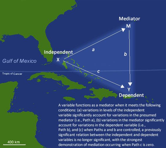
If you go to a consumer research conference, you will hear tales of how experiments have undergone particular statistical rites: the attainment of the elusive crossover interaction, the demonstration of full mediation through Baron and Kenny’s sacred procedure, and so on. DSN has nothing against any of these ideas, but is opposed to subjecting all ideas to the same experimental designs, to the same tests, the same alternative hypotheses (typically a null of no difference), and the same rituals.

Zhao, Lynch, and Chen point out in their recent Journal of Consumer Research article that Baron & Kenny’s Mediation Analysis is incredibly popular (ca 13,000 cites between 1986 and 2010), prescribed reflexively, though flawed in ways its users probably aren’t aware of. This article was invited by the journal “to serve as a tutorial on the state of the art in mediation analysis”.

ABSTRACT
Baron and Kenny’s procedure for determining if an independent variable affects a dependent variable through some mediator is so well known that it is used by authors and requested by reviewers almost reflexively. Many research projects have been terminated early in a research program or later in the review process because the data did not conform to Baron and Kenny’s criteria, impeding theoretical development. While the technical literature has disputed some of Baron and Kenny’s tests, this literature has not diffused to practicing researchers. We present a nontechnical summary of the flaws in the Baron and Kenny logic, some of which have not been previously noted. We provide a decision tree and a step-by-step procedure for testing mediation, classifying its type, and interpreting the implications of findings for theory building and future research.

REFERENCES
Baron, Reuben M. and David A. Kenny (1986), Moderator-Mediator Variables Distinction in Social Psychological Research: Conceptual, Strategic, and Statistical Considerations, Journal of Personality and Social Psychology, 51(6), 1173–82.

Bullock, J. G., Green, D. P, & Ha, S. E. (2010). Yes, But What’s the Mechanism? (Don’t Expect an Easy Answer), Journal of Personality and Social Psychology, Vol. 98, No. 4, 550–558.

Zhao, X., Lynch, J. G., Chen, Q. (2010).Reconsidering Baron and Kenny: Myths and Truths about Mediation Analysis. Journal of Consumer Research, 37, 197-206.

R Package for Causal Mediation Analysis

SPSS Code (see the Zhao, Lynch, and Chen article)

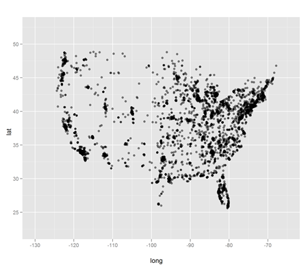
LATITUDE + LONGITUDE + OVERPLOTTING FIX = MAPS

Decision Science News is always learning stuff from colleague, physicist, mathlete, and all-around computer whiz Jake Hofman.

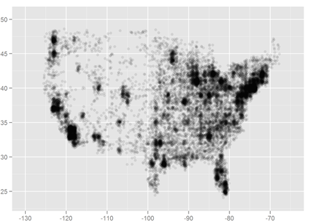
Today, it was a quick and clean way to make nice maps in R without using any map packages: just plot the latitude and longitude of your data points (e.g. web site visitors) along with the “alpha” parameter to allow for layering of coincident points. It’s duh in hindsight.

Above we see a how it looks with a little data. Below is the result with more data and a lower alpha:

In the words of James Taylor, all you have to do is call:

library(ggplot2)
qplot(long,lat,data=us,alpha=I(.1))

To get the Decision-Science-News-approved framing and aspect ratio for the USA:

qplot(long,lat,data=wtd,alpha=I(.1),
xlim=c(-125-10/2,-65),ylim=c(23.5,50.5)) +
opts(aspect.ratio = 3.5/5)

As we are certain that there are readers who will want to show that there are much nicer ways to do this, we say: download the data and show us.

HORMONE LINKED TO IN-GROUP GOODNESS, OUT-GROUP BADNESS

Who doesn’t like oxytocin? Who could dislike any substance referred to as a cuddle chemical? The answer may be you, if you are not in with the crowd feeling the effects of the hormone.

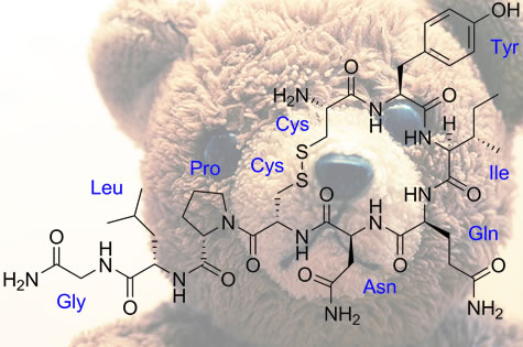
Carsten de Dreu and a super-long list of co-authors (listed below), have administered oxytocin to experimental participants and validated its bright side (cooperation among people in a group), but uncovered its dark side (defensive aggression towards people in other groups). Read all about it.

CITATION
Carsten K. W. De Dreu, Lindred L. Greer, Michel J. J. Handgraaf, Shaul Shalvi, Gerben A. Van Kleef, Matthijs Baas,Femke S. Ten Velden, Eric Van Dijk, Sander W. W. Feith. (2010) The Neuropeptide Oxytocin Regulates Parochial Altruism in Intergroup Conflict Among Humans. Science, 328(5984), 1408 – 1411.

ABSTRACT
Humans regulate intergroup conflict through parochial altruism; they self-sacrifice to contribute to in-group welfare and to aggress against competing out-groups. Parochial altruism has distinct survival functions, and the brain may have evolved to sustain and promote in-group cohesion and effectiveness and to ward off threatening out-groups. Here, we have linked oxytocin, a neuropeptide produced in the hypothalamus, to the regulation of intergroup conflict. In three experiments using double-blind placebo-controlled designs, male participants self-administered oxytocin or placebo and made decisions with financial consequences to themselves, their in-group, and a competing out-group. Results showed that oxytocin drives a “tend and defend” response in that it promoted in-group trust and cooperation, and defensive, but not offensive, aggression toward competing out-groups.

H/T author Michel Handgraaf
Photo credit 1: http://en.wikipedia.org/wiki/File:Oxytocin_with_labels.png
Photo credit 2: http://www.flickr.com/photos/markusschoepke/305865244/

QUIZ YOUR LOVED ONES ABOUT THEIR PROPENSITY TO PLAN

John Lynch, Richard Netemeyer, Stephen Spiller, Alessandra Zammit have recently published in the Journal of Consumer Research this article on the propensity to plan and financial well being

ABSTRACT

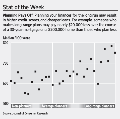
Planning has pronounced effects on consumer behavior and intertemporal choice. We develop a six-item scale measuring individual differences in propensity to plan that can be adapted to different domains and used to compare planning across domains and time horizons. Adaptations tailored to planning time and money in the short run and long run each show strong evidence of reliability and validity. We find that propensity to plan is moderately domain-specific. Scale measures and actual planning measures show that for time, people plan much more for the short run than the long run; for money, short- and long-run planning differ less. Time and money adaptations of our scale exhibit sharp differences in nomological
correlates; short-run and long-run adaptations differ less. Domain-specific adaptations predict frequency of actual planning in their respective domains. A “very long-run” money adaptation predicts FICO credit scores; low planners thus face materially higher cost of credit.

And while reading the article is fun, it’s also a hoot to take the propensity to plan test yourself, and give it to your friends and family. Give it a whirl, see if it accords with their behavior. Here are the items. Feel free to post your score in the comments.

For each question, answer on a scale from 1 to 6 in which 1 means “I strongly disagree” and 6 means “I strongly agree.”
Propensity to Plan for Money—Short Run:
1. I set financial goals for the next few days for what I
want to achieve with my money.
2. I decide beforehand how my money will be used in
the next few days.
3. I actively consider the steps I need to take to stick to
my budget in the next few days.
4. I consult my budget to see how much money I have
left for the next few days.
5. I like to look to my budget for the next few days in
order to get a better view of my spending in the future.
6. It makes me feel better to have my finances planned
out in the next few days.

Propensity to Plan for Money—Long Run:
1. I set financial goals for the next 1–2 months for what
I want to achieve with my money.
2. I decide beforehand how my money will be used in
the next 1–2 months.
3. I actively consider the steps I need to take to stick to
my budget in the next 1–2 months.
4. I consult my budget to see how much money I have
left for the next 1–2 months.
5. I like to look to my budget for the next 1–2 months
in order to get a better view of my spending in the
future.
6. It makes me feel better to have my finances planned
out in the next 1–2 months.

Propensity to Plan for Time—Short Run:
1. I set goals for the next few days for what I want to
achieve with my time.
2. I decide beforehand how my time will be used in the
next few days.
3. I actively consider the steps I need to take to stick to
my time schedule the next few days.
4. I consult my planner to see how much time I have left
for the next few days.
5. I like to look to my planner for the next few days in
order to get a better view of using my time in the
future.
6. It makes me feel better to have my time planned out
in the next few days.

Propensity to Plan for Time—Long Run:
1. I set goals for the next 1–2 months for what I want
to achieve with my time.
2. I decide beforehand how my time will be used in the
next 1–2 months.
3. I actively consider the steps I need to take to stick to
my time schedule in the next 1–2 months.
4. I consult my planner to see how much time I have left
for the next 1–2 months.
5. I like to look to my planner for the next 1–2 months
in order to get a better view of using my time in the
future.
6. It makes me feel better to have my time planned out
in the next 1–2 months.

ARTICLE TEXT [Download]

MEDIA MENTIONS
Wall Street Journal: http://jcr.wisc.edu/publicity/authors/docs/SUNJ.AA.1A020.A1.361Z2009.pdf

Yahoo Finance: http://finance.yahoo.com/retirement/article/109540/fast-track-to-financial-success

Decision Science News (meta-reference): http://www.decisionsciencenews.com/2010/06/18/the-propensity-to-plan-is-good-for-your-wallet/

GUESSING WHAT PEOPLE ARE THINKING ABOUT BASED ON BRAIN ACTIVATION

You know how in cheesy 80s movies and TV shows there will be a romantic scene, like two young people on a date, and the guy will say something like “I can read minds, you know” and the girl will say “Ok” and scrunch up her eyes and say “What am I thinking about now?” and then the guy will say something particularly cheesy?

Well, in the future they’ll be able to do that scene and the guy will say “apple” and the girl will go “that’s amazing!” and the guy will go “well, the base rate was one in 60” and the girl will go “can I get out of this fMRI now?”

In any case, read this by Marcel Just et al

A Neurosemantic Theory of Concrete Noun Representation Based on the Underlying Brain Codes

This article describes the discovery of a set of biologically-driven semantic dimensions underlying the neural representation of concrete nouns, and then demonstrates how a resulting theory of noun representation can be used to identify simple thoughts through their fMRI patterns. We use factor analysis of fMRI brain imaging data to reveal the biological representation of individual concrete nouns like apple, in the absence of any pictorial stimuli. From this analysis emerge three main semantic factors underpinning the neural representation of nouns naming physical objects, which we label manipulation, shelter, and eating … the fMRI-measured brain representation of an individual concrete noun like apple can be identified with good accuracy from among 60 candidate words, using only the fMRI activity in the 16 locations associated with these factors. To further demonstrate the generativity of the proposed account, a theory-based model is developed to predict the brain activation patterns for words to which the algorithm has not been previously exposed. The methods, findings, and theory constitute a new approach of using brain activity for understanding how object concepts are represented in the mind.

In order words, they can read your mind.

I like this task description:

Task: When a word was presented, the participants’ task was to actively think about the properties of the object to which the word referred.

… I wonder if the subjects were tempted to scrunch their eyes.

Find the full article here (free PDF download): http://www.plosone.org/article/info:doi/10.1371/journal.pone.0008622

REFERENCE: Just MA, Cherkassky VL, Aryal S, Mitchell TM (2010) A Neurosemantic Theory of Concrete Noun Representation Based on the Underlying Brain Codes. PLoS ONE 5(1): e8622. doi:10.1371/journal.pone.0008622

photo credit: The movie “Can’t Buy Me Love”, which doesn’t have the aforementioned scene, but does have the kind of nerdy-guy-dates-popular-girl device that causes writers to trot out the “I can read minds” bit.

PROS ARE NOT GETTING BETTER AT FREE THROWS

Rick Larrick recently told Decision Science News that baseball players have been getting better over the years in a couple ways.

First, home runs and strikeouts have increased. The careless or clueless reader might note that this is curious, for from the batter’s perspective home runs are a good thing and strikeouts are a bad thing. What’s going on? Batters may be swinging harder, increasing the chance of both. The purported improvement is a result of the benefit of a home run being greater than the cost of a strikeout. After all, a home run results in at least one run, often more, and runs are a big deal since the typical team earns only about 5 of them per game.

DSN wondered how the players learned to swing harder from one decade to the next. Was it based on feedback from coaches? Or from fans / media attention?

According to Larrick, the number of attempted stolen bases has decreased over the years. Apparently, it is only worth it to steal if one can pull a very high percentage of the time, higher than had been believed in previous years (anyone know the stat?). So while crowds (presumably) like the action of stolen bases, players do not respond by doing it more. Winning seems more important than pleasing the crowd, which is a strike against the fan-feedback hypothesis.

After our post on winning back-to-back baseball games, some folks like our friend Russ Smith made comparisons to the hot hand effect. There is something to it. However, in the baseball example one starts with a prior of .5 (since one doesn’t even know which two teams are playing), while in basketball the chance a pro will make a free throw is about .75 (since one can condition on the player being a pro). What is surprising is that in both cases, the past success tells you next to nothing.

This conversation lead your Editor to find this NY Times article which shows that, surprisingly, pro basketball players are not getting better at free throws over the years.

So, the question to the readers is: Why do some athletic abilities improve as history marches on (e.g., running speeds, batting, base-stealing) and others do not (e.g., free throws)?

P.S. For the record, Decision Science News is not becoming a sports blog. It is just a phase the Web site is going through. That said, there has been interest in seeing this kind of result in other sports, so that analysis will be coming in future posts, in glorious, glorious R and ggplot2. (Don’t know R yet? Learn by watching: R Video Tutorial 1, R Video Tutorial 2)

Photo credit: http://www.flickr.com/photos/cakecrumb/4398699952/. A cupcake was chosen because Jeff gave us empirical evidence that people like cupcakes much more than a control food.

COUNTERINTUITIVE PROBLEM, INTUITIVE REPRESENTATION

Blog posts about counterintuitive probability problems generate lots of opinions with a high probability.

Andrew Gelman and readers have been having a lot of fun with the following probability problem:

I have two children. One is a boy born on a Tuesday. What is the probability I have two boys? The first thing you think is “What has Tuesday got to do with it?” Well, it has everything to do with it.

DSN agrees with Andrew that one virtue of the “population-distribution” method is that it forces one to be explicit about various aspects of the problem, and in so doing, causes much confusion to disappear.

As a public service this week, Decision Science News presents the population-distribution representation of the problem (what it thinks of as the Gigerenzerian / Hoffragian / Peter Sedlmeier-ian representation of the problem) in a visual form.

To follow the logic, see Andrew’s post on how he solved the problem. Voila:

Red means “outside the reference class”. Yellow means “in the reference class but not boy-boy”. Green means “inside the reference class and boy-boy”.

Boy-boy in the reference class occurs with probability Green / (Green + Yellow) or 13 /27

NOTE
To see why DSN calls these Gigerenzerian / Hoffragian / Sedlmeierian representations, see:

Sedlmeier, P. (1997). BasicBayes: A tutor system for simple Bayesian inference.
Behavior Research Methods, Instruments & Computers, 29(3), 328-336.

Gigerenzer, G., & Hoffrage, U. (1995). How to improve Bayesian reasoning without instruction: Frequency formats. Psychological Review, 102,, 684–704.

(Sorry for not using R, excel is just darn fast for some things)

IMAGINING THE FUTURE TO HELP PREPARE FOR IT

The New York Times just ran a piece called Some Novel Ideas for Improving Retirement Income about having people read Victorian novels in order to increase their retirement savings rates.

Actually, that is not true.

But it did feature some newer ideas from Psychology and Behavioral Finance and Economics presented at a Allianz-sponsored event on Monday in NYC on improving retirement decision making, including:

• Work by Hal Ersner-Hershfield, Dan Goldstein, and Bill Sharpe using age-morphed photos of people with varying emotional expressions as a way to increase how connected people feel to their future selves. It is like the scene in a Christmas Carol in which Scrooge sees the future and upon returning promises: “I will live in the Past, the Present, and the Future. The Spirits of all Three shall strive within me. I will not shut out the lessons that they teach.” Like the Distribution Builder, this technology helps people imagine what the future may be like.

Hal, sad about saving now, but psyched about spending later

• Work by Eric Johnson on high sensitivity to loss among the elderly
• Findings by Alessandro Previtero on how recent stock market returns affect people’s decisions to buy annuities (which of course last a long, long time)
• Ideas by George Loewenstein on using mental accounts to help people achieve goals

These projects and more can be read about in the new report from Allianz entitled Behavioral Finance and the Post-Retirement Crisis.

photo credit: www.flickr.com/photos/nrg-photos/4199392655