Area plots unmasked
 Subscribe to Decision Science News by Email (one email per week, easy unsubscribe)
RESULTS OF THE GREAT AREA PLOT QUIZ
If you are the type of reader who remembers things from last week, you may remember the great area plot quiz we had running.
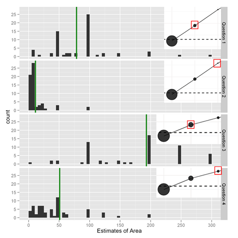
This week, we are excited to announce that the results are in. The plot above shows answers to the four questions. The correct answers are indicated with the green lines. Remember, in each question, the big circle was area 1000 and readers had to guess the areas of the second and third biggest circles.
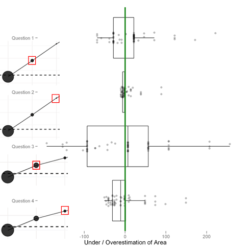
As the above plot shows, when the circles are 8% to 20% of the size of the biggest (questions 1 and 3), people exhibit a great deal of variation in their area estimates, but the responses benefit from some “wisdom of crowds” magic and approximate the truth. When the circles are 5% or 1% of the biggest, people tend to underestimate the area. It is also interesting to note that 1) the biggest variation in response is in the question with the biggest circle; this was a somehing surprise, since one would think it would be easier to visualize putting a biggish circle inside a little one, however floor effects can account for some of it 2) While the circles in questions 1 and 4 weren’t that different in area, people treated them somewhat differently. It seems as if in question 4, the fact the circle was third largest caused people to underestimate its size. Perhaps if it were second largest, it may have been spot on. The mean absolute deviations from the correct answer in Questions 1 – 4 were 38.6, 9.4, 73.6, and 31.2 respectively.
The following plot, which shows the difference between the responses and the correct answers, is also informative (and frankly, we couldn’t decide which one to lead with). It makes the underestimation apparent.
Hadley of ggplot2-authoring fame asked if we used “scale_area” to make our plots. Yes, we did.
p <- ggplot(plot.data, aes(num.contacts.sales.part1,response))

p <- p + geom_point(aes(size=count,alpha=.8)) + geom_line(size=.25)

p <- p + scale_area(to=get.range(plot.data$count))
where
get.range <- function(counts) {

dist <- counts/sum(counts)

my.range <- c(sqrt(min(dist)*100),sqrt(max(dist)*100))

my.range <- round(my.range,1)

}
Naturally, at this point, many R-hounds will want to play with the data. There are many things to try, such as computing the accuracy of the third circles on the assumption that the areas of the second circles are all correct. Far be it from us to stand in the way of such tinkering. Just paste the following into an R session to reproduce the data frame “df” with the responses.
df=structure(list(variable=structure(c(1L,1L,1L,1L,1L,1L,1L,1L,1L,1L,

1L,1L,1L,1L,1L,1L,1L,1L,1L,1L,1L,1L,1L,1L,1L,1L,1L,1L,1L,1L,1L,1L,1L,

1L,1L,1L,1L,1L,1L,1L,1L,1L,1L,1L,1L,1L,1L,1L,1L,1L,1L,1L,1L,1L,1L,1L,

1L,1L,1L,1L,1L,1L,1L,1L,2L,2L,2L,2L,2L,2L,2L,2L,2L,2L,2L,2L,2L,2L,2L,

2L,2L,2L,2L,2L,2L,2L,2L,2L,2L,2L,2L,2L,2L,2L,2L,2L,2L,2L,2L,2L,2L,2L,

2L,2L,2L,2L,2L,2L,2L,2L,2L,2L,2L,2L,2L,2L,2L,2L,2L,2L,2L,2L,2L,2L,2L,

2L,2L,2L,3L,3L,3L,3L,3L,3L,3L,3L,3L,3L,3L,3L,3L,3L,3L,3L,3L,3L,3L,3L,

3L,3L,3L,3L,3L,3L,3L,3L,3L,3L,3L,3L,3L,3L,3L,3L,3L,3L,3L,3L,3L,3L,3L,

3L,3L,3L,3L,3L,3L,3L,3L,3L,3L,3L,3L,3L,3L,3L,3L,3L,3L,3L,3L,3L,4L,4L,

4L,4L,4L,4L,4L,4L,4L,4L,4L,4L,4L,4L,4L,4L,4L,4L,4L,4L,4L,4L,4L,4L,4L,

4L,4L,4L,4L,4L,4L,4L,4L,4L,4L,4L,4L,4L,4L,4L,4L,4L,4L,4L,4L,4L,4L,4L,

4L,4L,4L,4L,4L,4L,4L,4L,4L,4L,4L,4L,4L,4L,4L,4L),.Label=c("q1","q2",

"q3","q4"),class="factor"),value=c(50,60,70,50,10,100,40,50,50,50,100,

100,100,50,50,111,100,150,10,250,70,65,100,200,100,100,100,40,100,20,

50,200,100,100,50,100,125,100,100,100,50,100,100,10,100,200,100,100,

63,100,100,100,80,10,50,80,50,125,50,300,100,50,150,50,5,5,7,5,2,10,1,

25,8,5,10,10,20,5,1,7,10,50,1,100,8,5,10,50,10,10,10,8,10,2,5,50,15,10,

2,5,16,10,25,10,5,10,10,1,10,25,10,25,6,10,10,10,12,1,10,10,5,30,5,100,

10,5,20,3,100,200,200,100,200,250,200,100,90,50,150,300,200,100,100,

250,250,300,100,400,120,120,250,300,250,200,250,200,200,40,100,400,130,

200,100,200,250,300,200,200,100,150,200,40,250,450,250,200,169,100,1,

250,200,50,200,160,200,250,100,400,300,100,300,100,10,50,40,25,20,125,

40,25,15,5,20,150,100,25,20,28,50,100,10,200,15,25,25,100,60,20,125,40,

40,4,10,100,25,50,10,20,63,30,50,50,10,50,50,10,60,200,50,50,42,10,0.1,

62,40,5,50,25,50,125,20,100,30,50,60,20)),.Names=c("variable","value"),

class="data.frame",row.names=c(NA,-256L))
If you want the correct answers (what we in JDM call the “normative” answers), just paste this, too.
df$norm=c(rep(78.4 ,nrow(df)/4),

rep( 11.2,nrow(df)/4),

rep(193.1,nrow(df)/4),

rep(50.9,nrow(df)/4))


I have been looking forward to seeing the results, and I think that there are two lessons.
1) If you want to convey information to an audience, don’t use the area or diameter of anything, as audience members will incorrectly estimate the quantitative information by up to a factor of four. We might expect this result based on Cleveland’s model for how we interpret graphs, as areas, diameters and angles all defeat the table look-up operation that yields quantitative information. Conversely, the disks do support the pattern perception operation, providing a clear ranking of smaller-to-larger disks.
2) If the goal is to estimate the size of an unknown geometrical figure, you can use the “wisdom of crowds” to get a pretty good estimate. Perhaps this should not be surprising, as the way these graphs were set up encourages the audience to make comparisons between differently-sized shapes, much the same as in Saaty’s Analytical Hierarchy Process (AHP), which I have seen produce remarkably accurate estimations. Using the more direct pair-wise comparisons and the mathematics of AHP would probably have resulted in a better estimate of the area of each of the disks.
December 21, 2010 @ 4:22 am