Decision Science News

SAMPLE UNTIL THE FIRST SUCCESS, PUT A CONFIDENCE INTERVAL ON P(SUCCESS)

We wrote last week of Charles Darwin’s love of the “rule of three” which, according to Stigler “is simply the mathematical proposition that if a/b = c/d, then any three of a, b, c, and d suffice to determine the fourth.”

We were surprised to learn this is called the rule of three, as we had only heard of the rule of three in comedy. We were even more surprised when a reader wrote in telling us about a rule of three in statistics. According to Wikipedia: the rule of three states that if a certain event did not occur in a sample with n subjects … the interval from 0 to 3/n is a 95% confidence interval for the rate of occurrences in the population.

It’s a heuristic. We love heuristics!

We decided to give it a test run in a little simulation. You can imagine that we’re testing for defects in products coming off of a production line. Here’s how the simulation works:

• We test everything that comes off the line, one by one, until we come across a defect (test number n+1).
• We then make a confidence interval bounded by 0 and 3/n and make note of it. In the long run, about 95% of such intervals should contain the true underlying probability of defect.
• Because it’s a simulation and we know the true underlying probability of defect, we make note of whether the interval contains the true probability of defect.
• We repeat this 10,000 times at each of the following underlying probabilities: .001, .002, and .003.

Let’s work through and example. Suppose you watch 1,000 products come off the line without defects and you see that the 1,001st product is defective. You plug n=1000 into 3/n and get .003, making your 95% confidence interval for the probability of a defective product to be 0 to .003.

The simulation thus far assumes the testers have the patience to keep testing until they find a defect. In reality, they might get bored and stop testing before the first defect is found. To address this, we also simulated another condition in which the testing is stopped at n/2, halfway before the first defect is found. Of course, people have no way of knowing when if they are half the way to the first defective test, but our simulation can at least let us know what kind of confidence interval one will get if one does indeed stop halfway.

Here’s the result on bracketing, that is, how often the confidence intervals contain the correct value:

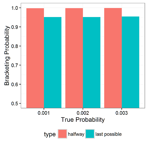
Across all three levels of true underlying probabilities, when stopping immediately before the first defect, we get 95% confidence intervals. However, when we stop half way to the first defect, we get closer to 100% intervals (99.73%, 99.80%, and 99.86%, respectively).

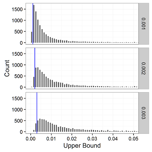
So we know that the upper bounds of these confidence intervals fall above the true probability 95% to about 99.9% of the time, but where do they fall?

In the uppermost figure of this post, we see the locations of the upper bounds of the simulated confidence intervals when we stop immediately before the first defect. For convenience, we draw blue lines at the true underlying probabilities of .001 (top), .002 (middle), and .003 (bottom). When it’s a 95% confidence interval, about 95% of the upper bounds should fall to the right of the blue line, and 5% to the left. Note that we’re zooming into to cut the X axis at .05 so you can actually see something. Keep in mind it extends all the way to 1.0, with the heights of the bars trailing off.

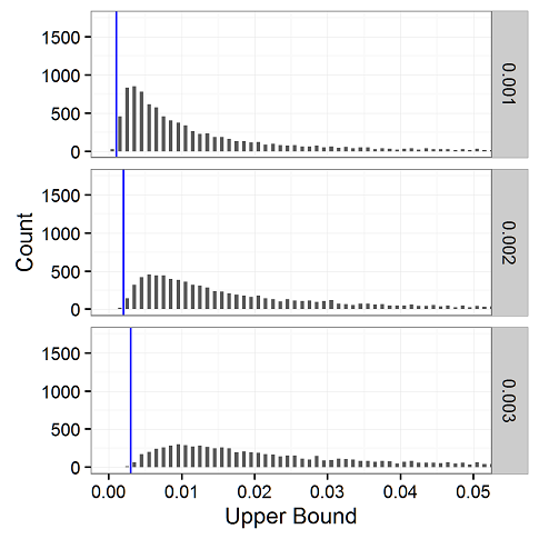
For comparison, let’s look at the case in which we stop halfway to the first defect. As suggested by the bracketing probabilities, here we see almost all of the upper bounds exceed the true underlying probabilities. As our applied statistician reader wrote us about the rule of three, “the weakness is that in some situations it’s a very broad confidence interval.”

REFERENCE
A Look at the Rule of Three
B. D. Jovanovic and P. S. Levy
The American Statistician
Vol. 51, No. 2 (May, 1997), pp. 137-139
DOI: 10.2307/2685405
Stable URL: http://www.jstor.org/stable/2685405

R CODE FOR THOSE WHO WANT TO PLAY ALONG AT HOME

require(scales)
library(ggplot2)
library(dplyr)
levels = c(.001,.002,.003)
ITER = 10000
res_list = vector('list', ITER*length(levels))
index=1
for(true_p in levels) {
for (i in 1:ITER) {
onesam = sample(
x = c(1, 0),
size = 10*1/true_p,
prob = c(true_p, 1 - true_p),
replace = TRUE
)
cut = which.max(onesam) - 1
upper_bound_halfway = min(3 / (cut/2),1)
upper_bound_lastpossible = min(3/cut,1)
res_list[[index]] =
data.frame(
true_p = true_p,
cut = cut,
upper_bound_halfway = upper_bound_halfway,
bracketed_halfway = true_p < upper_bound_halfway,
upper_bound_lastpossible = upper_bound_lastpossible,
bracketed_lastpossible = true_p < upper_bound_lastpossible ) index=index+1 }}
df = do.call('rbind',res_list)
rm(res_list)
plot_data = rbind(
df %>% group_by(true_p) %>% summarise(bracketing_probability = mean(bracketed_halfway),type="halfway"),
df %>% group_by(true_p) %>% summarise(bracketing_probability = mean(bracketed_lastpossible),type="last possible")
)
plot_data
p=ggplot(plot_data,
aes(x=true_p,y=bracketing_probability,group=type,fill=type)) +
geom_bar(stat="identity",position="dodge") +
coord_cartesian(ylim=c(.5,1)) +
theme_bw() +
theme(legend.position = "bottom",
panel.grid.minor.x = element_blank()) +
labs(x="True Probability",y="Bracketing Probability")
p
ggsave(plot=p,file="bracketing.png",width=4,height=4)
plot_data2 = df %>%
dplyr::select(-bracketed_halfway,-bracketed_lastpossible) %>%
tidyr::gather(bound_type,upper_bound,c(upper_bound_halfway,upper_bound_lastpossible)) %>%
arrange(bound_type,upper_bound) %>%
mutate(bin = floor(upper_bound/.001)*.001) %>%
group_by(bound_type,true_p,bin) %>%
summarise(count = n()) %>%
ungroup()
p=ggplot(subset(plot_data2,bound_type=="upper_bound_lastpossible"),aes(x=bin+.0005,y=count)) +
geom_bar(stat="identity",width = .0005) +
geom_vline(aes(xintercept = true_p),color="blue") +
coord_cartesian(xlim = c(0,.05)) +
labs(x="Upper Bound",y="Count") +
facet_grid(true_p ~ .) +
theme_bw() +
theme(legend.position = "none")
p
ggsave(plot=p,file="upper_bound_lastpossible.png",width=4,height=4)
#repeat for upper_bound_halfway
p=ggplot(subset(plot_data2,bound_type=="upper_bound_halfway"),
aes(x=bin+.0005,y=count)) +
geom_bar(stat="identity",width = .0005) +
geom_vline(aes(xintercept = true_p),color="blue") +
coord_cartesian(xlim = c(0,.05),ylim=c(0,1750)) +
labs(x="Upper Bound",y="Count") +
facet_grid(true_p ~ .) +
theme_bw() +
theme(legend.position = "none")
p
ggsave(plot=p,file="upper_bound_halfway.png",width=4,height=4)