Can’t compute the standard deviation in your head? Divide the range by four.
TESTING A HEURISTIC TO ESTIMATE STANDARD DEVIATION
Click to enlarge
Say you’ve got 30 numbers and a strong urge to estimate their standard deviation. But you’ve left your computer at home. Unless you’re really good at mentally squaring and summing, it’s pretty hard to compute a standard deviation in your head. But there’s a heuristic you can use:
Subtract the smallest number from the largest number and divide by four
Let’s call it the “range over four” heuristic. You could, and probably should, be skeptical. You could want to see how accurate the heuristic is. And you could want to see how the heuristic’s accuracy depends on the distribution of numbers you are dealing with.
Fine.
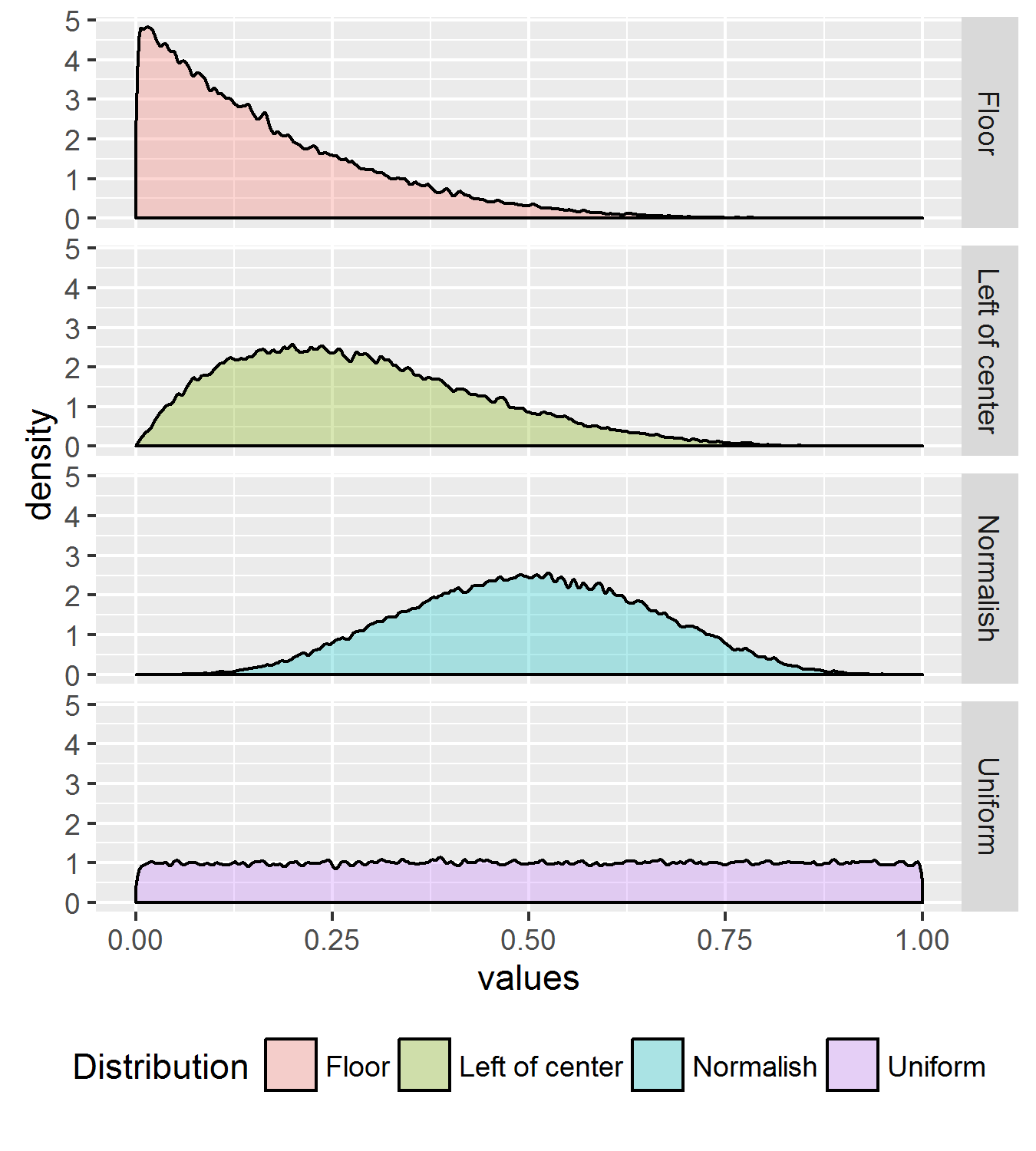
We generated random numbers from four distributions, pictured above. We nickname them (from top to bottom): floor, left of center, normalish, and uniform. They’re all beta distributions. If you want more detail, they’re the same beta distributions studied in Goldstein and Rothschild (2014). See the code below for parameters.
We vary two things in our simulation:
1) The number of observations on which we’re estimating the standard deviation.
2) The distributions from which the observations are drawn
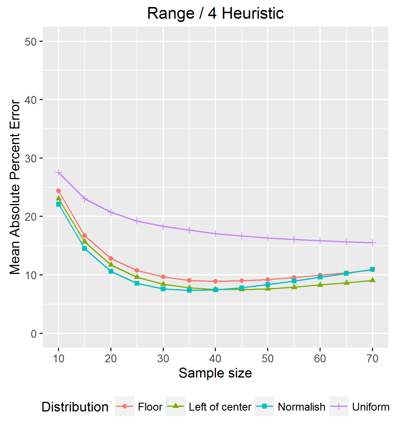
With each sample, we compute the actual standard deviation and compare it to the heuristic’s estimate of the standard deviation. We do this many times and take the average. Because we like the way mape sounds, we used mean absolute percent error (MAPE) as our error metric. Enough messing around. Let’s show the result.
Click to enlarge
There you have it. With about 30 to 40 observations, we could get an average absolute error of less than 10 percent for three of our distributions, even the skewed ones. With more observations, the error grew for those distributions.
With the uniform distribution, error was over 15 percent in the 30-40 observation range. We’re fine with that. We don’t tend to measure too many things that are uniformly distributed.
Another thing that set the uniform distribution apart is that its error continued to go down as more observations were added. Why is this? The standard deviation of a uniform distribution between 0 and 1 is 1/sqrt(12) or 0.289. The heuristic, if it were lucky enough to draw 1 and a 0 as its sample range, would estimate the standard deviation as 1/4 or .25. So, the sample size increases, the error for the uniform distribution should drop down to a MAPE of 13.4% and flatten out. The graph shows it is well on its way towards doing so.
REFERENCES
Browne, R. H. (2001). Using the sample range as a basis for calculating sample size in power calculations. The American Statistician, 55(4), 293-298.
Hozo, S., Djulbegovic, B., & Hozo, I. (2005). Estimating the mean and variance from the median, range, and the size of a sample. BMC medical research methodology, 5(1), 1.
Ramıreza, A., & Coxb, C. (2012). Improving on the range rule of thumb. Rose-Hulman Undergraduate Mathematics Journal, 13(2).
Wan, X., Wang, W., Liu, J., & Tong, T. (2014). Estimating the sample mean and standard deviation from the sample size, median, range and/or interquartile range. BMC medical research methodology, 14(1), 135.
Want to play with it yourself? R Code below. Thanks to Hadley Wickham for creating tools like dplyr and ggplot2 which take R to the next level.

Shouldn’t you test this with unbounded distributions too, like normal, lognormal, etc? And also go over a larger range of sample numbers? With unbounded distributions I imagine the estimate gets really bad as the number of samples increases. I think it’s a neat heuristic, but I’d like to understand when it can’t be applied.
June 18, 2016 @ 11:56 am
Great questions! See the references at the end for more thorough treatments.
June 18, 2016 @ 12:09 pm
Check out what happens with some unbounded distributions and other real data here… http://asinayev.github.io/how-good-is-the-standard-deviation-range-divided-by-four-rule.html
June 19, 2016 @ 7:14 pm
See also the references for an even more comprehensive analysis.
June 19, 2016 @ 7:24 pm
I’ve looked at this across a range of real-world data sets obtained through my day job, and find that a divisor of 5 tends to be more robust (results in a MAPE lower by 10% to 20%) than a divisor of 4. That’s far from _all_ data sets, of course, but I have used data sets ranging from nearly-normal to highly skewed (skewness = 0.1 to 10) and data sets with small and large n (n = 6 to about 50,000).
Is 4 recommended because it’s a simpler divisor than 5, or because 4 was derived from theoretic pdfs like those used in this post?
June 19, 2016 @ 7:47 pm