Judgment and Decision Making, Vol. 17, No. 5, September 2022, pp. 1146-1175
Sample decisions with description and experience
Ronald Klingebiel* #
Feibai Zhu#
|
Abstract: Decision makers weight small probabilities differently when sampling them and when seeing them stated. We disentangle to what extent the gap is due to how decision makers receive information (through description or experience), the literature’s prevailing focus, and what information they receive (population probabilities or sample frequencies), our novel explanation. The latter determines statistical confidence, the extent to which one can know that a choice is superior in expectation. Two lab studies, as well as a review of prior work, reveal sample decisions to respond to statistical confidence. More strongly, in fact, than decisions based on population probabilities, leading to higher payoffs in expectation. Our research thus not only offers a more robust method for identifying description-experience gaps. It also reveals how probability weighting in decisions based on samples — the typical format of real-world decisions — may actually come closer to an unbiased ideal than decisions based on fully specified probabilities — the format frequently used in decision science.
Keywords: decisions based on samples, description-experience gap, decisions from experience, weighting of small probabilities, statistical reasoning, choice under risk and uncertainty
1 Introduction
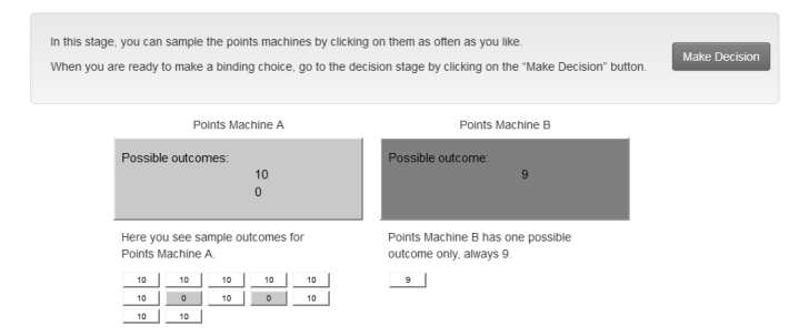
Many real-world decisions are based on samples, some small, some big, but none infinitely so. Therefore, inferences about the true state of nature are necessary. A manager might, for example, face the business decision stylized in Figure 1. Either she decides to continue with her firm’s existing product, for a more or less guaranteed return of $2m, or she invests in making a risky new product. In her business experience, she has observed one other firm’s launch of the new product returning $12m, while four other firms had their new product return $0.
| Figure 1: Canonical choice-set format. Opting for the safe choice would underweight the small probability of success in the risky choice. |
Whether or not the manager foregoes the old product and launches the new product depends on her weighting of the small chance of success. Research suggests that people underweight such rare-event probabilities more often when they receive their information through sampling experience, as our manager does, than when they base their decisions on described probabilities (HertwigErev, 2009,Wulff et al., 2018).
The canonical lab experiment rendering this description-experience gap (DE-Gap) compares the decisions of people who know that a percentage of draws from each lottery is successful, with those of people who sample the lotteries and happen to observe some draws to be successful and others not. Objectively, samplers are afforded less certainty of whether or not one lottery is better than another in expectation, than decision makers who receive fully specified probabilities for lotteries’ underlying outcome probabilities (de Palma et al., 2014).
This difference between treatments can be objectively quantified. Statistical confidence — the posterior probability of a rare event that makes one choice superior to its alternative in expectation — ranges between 0 and 1 (Bayes et al., 1763,Hill, 1968). Assuming an uninformed prior, the five sample draws (four new-product failures, one success) in an experience-treatment implementation of our product-decision example afford 26% statistical confidence in the expected value of the old product exceeding that of the new product alternative. This would fall to 22% if the sample size were ten times larger and the proportion of success unchanged. A description treatment with a stated success probability of 20%, however, would provide exactly 0% statistical confidence that the old product offers superior value in expectation (see Table 1).
| Table 1: Statistical Confidence in Experimental Treatments |
Treatments | Risky Alternatives to a Safe $2 | Source | Statistical Confidence |
|
20.25@percentExperienced Samples | Outcomes | $0 | $12 | | 20.25@percentp(EVUW ≥ EVAlt)=0.26 |
|
| | Drawn sample | 4 | 1 | | |
|
20.25@percentDescribed Samples | Outcomes | $0 | $12 | 20.25@percentYoked description condition, mirroring the statistical properties of the experience condition | 20.25@percentp(EVUW ≥ EVAlt)=0.26 |
|
| | Stated sample | 4 | 1 | | |
|
20.25@percentDescribed Probabilities | Outcomes | $0 | $12 | 20.25@percentYoked version of the description condition used in DE-Gap studies (Wulff et al., 2018) | 20.25@percentp(EVUW ≥ EVAlt)=0 |
|
| | Stated probabilities | 80% | 20% | | |
|
[para,flushleft]
Notes. Statistical confidence p(EVUW ≥ EVAlt) denotes the likelihood p that the underlying probability of a risky outcome is such that the expected value EV of the as-if-underweighting choice UW exceeds that of an alternative choice Alt. In the example, the safe prospect of $2 constitutes the as-if-underweighting choice. By choosing as if they underweight, decision makers are better off in expectation only if the underlying probability for the $12 outcome is approximately 16.7% or lower. See Section 3 for a formal derivation of statistical confidence.
If statistical confidence in the underweighting choice1 is zero in a description treatment and greater than zero in an experience treatment, as illustrated with the product-decision example, it is easy to imagine that description-treatment subjects less likely choose as if they underweight than experience-treatment subjects. In other cases, the description-treatment probability that the underweighting choice is superior to the alternative is 1, and the experience-treatment posterior is below 1. Choosing as if underweighting might then be less likely in experience treatments than description treatments.
DE-Gap studies entail varying amounts of either mismatch in statistical confidence between treatments. Underweighting found in the treatments may thus balance out, yield a positive gap, or a negative gap, on average. Not surprisingly, research reports negative (e.g., Glöckner et al., 2016), positive (e.g., Ungemach et al., 2009), as well as insignificant (e.g., CamilleriNewell, 2011b) overall DE-Gaps. Therefore, it is important to disentangle to what extent DE-Gaps are caused by differences in statistical confidence between sample and population statistics as opposed to differences in the process of attaining information through description and experience.
We introduce an experimental design for separating these differences. We first ascertain the typical DE-Gap between an Experienced-Sample treatment and a Described/Probabilities treatment, using a yoked version of the classic design that is robust to sampling error and amplification (HertwigPleskac, 2010). We then add a treatment describing samples (see Table 1), rather than populations. The only difference between the new Described-Samples treatment and a conventional Experienced-Samples treatment is the subjects in the latter sample themselves, whereas subjects in the former receive a sample record. The new treatment thus entails inference but not experience.
For the literature’s five canonical choice sets (see Table 2), we find that experiencing samples leads to choices that imply a lower weighting of small probabilities than seeing descriptions of the same samples, an effect that can be ascribed to differences in how information is attained. We also find lower weights for small probabilities in decisions based on described samples than decisions based on described probabilities, an effect that can be ascribed to differences in what information is attained. We replicate this finding in two experiments, using both group-mean difference tests and model-fitting approaches.
Econometric analysis then offers detail on the gap between described samples and described probabilities. Sample decisions display strong sensitivity to statistical confidence. If sample confidence exceeds the zero confidence of yoked decisions with described probabilities, underweighting is higher. If sample confidence is lower than the full confidence of yoked decisions with described probabilities, underweighting is lower. Interestingly, when statistical confidence is comparable across treatments, sample decisions prove more sensitive: Near zero confidence, sample decisions underweight less, and near full confidence, they underweight more. Decision makers thus place lower weights on events when sample evidence strongly suggests them to be rare than when stated probabilities confirm them to be so, and vice versa. As a result, sample subjects end up maximizing their payoff more often.
Our work, therefore, helps explain portions of previously reported DE-Gaps (Rakow et al., 2008,CamilleriNewell, 2019) and additionally informs theory on decision making under uncertainty (EinhornHogarth, 1985,Baillon et al., 2017,Erev et al., 2017,Kutzner et al., 2017). Sample decisions appear sensitive to statistical confidence in the desirability of risky choices, more so than decisions based on full information.
2 Risky Choice with Description and Experience
Decision makers seldom receive information that fully specifies the probabilities of realizing the outcomes of decision alternatives, but rather have to infer this information from whatever samples they may have observed in the past. Experimental designs explicitly aiming to capture such settings (starting with BarronErev, 2003,Hertwig et al., 2004,Weber et al., 2004) ask subjects to choose between two lotteries. Typically, the single possible outcome of a safe lottery falls in between the two possible outcomes of another, risky lottery, one outcome of which occurs rarely. This design mirrors the stylized opening example of the manager observing outcomes for old and new products before investing in one herself. Choices observed in the lab reveal that people behave as if they underweight rare outcomes when they learn about probabilities through sampling experience. When people receive probability descriptions, they underweight less or even overweight (KahnemanTversky, 1979). This gap in underweighting is understood as the description-experience gap.
Statistical features of a sampling contexts that have already been shown to explain parts of the DE-Gap include sampling error and amplification as well as sampling-space awareness. When subjects draw samples from two money machines before deciding which to play for money, many stop early (HertwigErev, 2009,Hau et al., 2010). The experienced outcome frequencies can, therefore, differ substantially from money-machines’ underlying probabilities. Over- and under-sampling rare events is common. Some subjects might even sample only the rare event or no rare events at all.
As a consequence of such sampling errors, the mean of experienced sample outcomes for a risky choice differs from the outcome of a safe alternative more strongly in experience treatments than the choice means do in description treatments (HertwigPleskac, 2010). Coupled perhaps with a tendency to overestimate the representativeness of small samples (TverskyKahneman, 1971), this expected-value amplification then engenders decision behavior that departs from behavior observed in description treatments.
Sampling error can be eliminated by mandating a fixed amount of sampling (Ungemach et al., 2009,CamilleriNewell, 2011a,AydoganGao, 2020), incentivizing prolonged sampling (e.g., Hau et al., 2008), or making description probabilities reflect experienced frequencies, in a process called yoking (Rakow et al., 2008,Hau et al., 2010,HertwigPleskac, 2010). These studies show heterogeneous results: the gap persists in some studies (e.g., Jessup et al., 2008,CamilleriNewell, 2011a) and disappears in others (e.g., Rakow et al., 2008). In the absence of sampling error, the average description-experience gap is smaller (Wulff et al., 2018).
Experimenters also often keep experience-treatment subjects unaware of the sample space. No information is provided about the number and the magnitude of possible outcomes for the money machine that is to be sampled. This sample-space unawareness introduces information asymmetry with description-treatment subjects (HadarFox, 2009). Experience-treatment subjects can learn about possible outcomes only during sampling, and some do not draw a rare outcome. They thus naturally underweight the possibility of its existence (de Palma et al., 2014).2 Conversely, if subjects do happen to draw two different outcomes for one machine, they may expect the alternative machine to have multiple outcomes too. What looks like underweighting of a rare event may actually be overweigthing of a non-existent event (Glöckner et al., 2016,HeDai, 2022).3 Studies that explicitly stated sample spaces to participants found little underweighting and even overweighting (Erev et al., 2008,HadarFox, 2009).
Behavioral explanations for the description-experience gap in settings without feedback4 center on recency, order, and primacy effects that are at play when people receive information iteratively, rather than in summary form. More recent draws have a stronger influence on decision making than earlier draws that might fade from memory (e.g., Stewart et al., 2006,BarronYechiam, 2009,Rakow et al., 2010,Kopsacheilis, 2018). Since rare events occur less often, they are less often part of the most recent set of sample draws. In the absence of yoking, subjects may additionally use heuristics for when to stop sampling that can produce recency effects (Wulff et al., 2018). Beyond recency, it sometimes matters which outcome is drawn first (RakowRahim, 2010) and in which order outcomes are drawn thereafter, with rare occurrences being processed disadvantageously (HogarthEinhorn, 1992).
Our work proposes the novel mechanism of statistical confidence as an explanation of DE-Gaps, even if these were observed in yoked and otherwise carefully controlled settings. When sampling error is absent and sample frequencies match stated probabilities, the statistical properties of decision problems in experience treatments continue to differ from those in description treatments, requiring inference. And where inferred and stated probabilities differ, gaps in decision behavior may occur. We provide an experimental design that permits separation of DE-Gaps’ inference component, driven by variation in statistical confidence in the information that is attained, from the experience component, driven by variation in the process with which information is attained.
3 Statistical Confidence and As-If-Underweighting Behavior
Previous studies compare description treatments containing fully specified probabilities with experience treatments containing samples from which probabilities can only be inferred. In experience treatments, subjects learn about sample frequencies that can help estimate underlying probabilities, albeit imprecisely, as per Bayes’ theorem (Bayes et al., 1763). But no matter how long subjects sample and how many samples they draw, they cannot identify the underlying probabilities as fully as their counterparts in description treatments. This is true even in the absence of sampling error and amplification, that is when described probabilities mirror sampling frequencies. Sample-treatment subjects are thus afforded different statistical confidence in whether or not the expected payoff from an as-if-underweighting choice exceeds that of the alternative choice.
Statistical confidence is a property of the decision problem and can be understood as the posterior likelihood of a desired outcome distribution given sample draws (e.g., Hill, 1968,Laplace, 1986). Statistical confidence is not to be mistaken for people’s subjective confidence in outcome probabilities (BazermanMoore, 2013,LejarragaLejarraga, 2020). Exact elicitation of the latter is hard and not a concern of this paper.5 Instead, even with subjective confidence unknown, we can observe to which extent choice behavior varies with decision problems’ statistical properties such as posterior likelihood.6
There are multiple ways of calculating statistical confidence, including those based on Bayesian inference (cf. PiresAmado, 2008) and frequentist statistics (cf. Brown et al., 2001). Their suitability differs slightly in limit cases, due to different assumptions about priors and functional forms. An evaluation of their computational efficacy would go beyond the confines of this paper. Important for our purposes is that any method values statistical confidence strictly between 0 and 1 in sample situations, and exactly 0 or 1 for fully described probabilities.
To illustrate how posteriors can influence choice behavior, we derive the statistical confidence that the manager in the opening decision example could have in the superiority of a choice that would be classified as-if-underweighting in DE-Gap studies (cf. Wulff et al., 2018). The manager observed new-product performance on five occasions, one rendering a successful outcome of $12m and four rendering unsuccessful outcomes of $0. The alternative to the risky new product return is the old-product’s safe return of $2m. Choosing the old-product (safe) would be as if she underweighted the small probability of a high new-product return (risky). If by contrast our example problem were one with a small probability of a low outcome, the risky choice would be labeled as underweighting instead (and our example calculations reversed).
A risk-neutral manager would choose the safe old product if its expected value exceeded that of the risky new product (EVUW ≥ EVAlt). This is the case when the underlying probability of the high new-product outcome p($12m) is smaller than 16.7%. The conditional probability of p($12m) being no larger than 16.7% (Event A) given the sample for five draws (Event B) can be expressed with Bayes’ theorem
Pr(A|B) = Pr(B|A) Pr(A)/Pr(B).
We assume for now that investing in a new product is a Bernoulli trial (as our experimental lotteries indeed are). Let y denote the number of successful outcomes and n denote the number of draws. So the probability of observing one successful outcome in five draws can be stated as
p(y|θ)= n yθ^y(1-θ)^n-y,
with p(θ) being the set of possible probabilities between 0 and 1. We assume that the manager had a uniform prior over all those possible probabilities: p(θ)∼ U(0,1). We thus have the proportionality
p(θ|y) ∝θ^y(1-θ)^n-y.
The posterior density θy(1−θ)n−y is beta distributed (BernardoSmith, 1994,BolstadCurran, 2016), specifically
θ|y∼Beta(y+1, n-y+1).
Knowing n and y, we can compute the statistical confidence in the expected return of the old product being greater than that of the new product (p(EVUW ≥ EVAlt )= F(0.167;2,5) = 0.26; F denotes the cumulative distribution function). Given her sample experience, the manager can be 26% confident that the new product will have a success rate of below 16.7%, at which point the old product becomes the better choice. By comparison, another risk-neutral manager, who is told that the new-product success rate is exactly 20%, would have statistical confidence of 0 that the old product is the better choice in expectation. One who is told that the new-product success rate is a guaranteed 10%, would be 100% confident, statistically, that the old product yields more in expectation than the new product. Sample subjects’ statistical confidence, by contrast, is strictly bigger than 0 and strictly smaller than 1 for any frequency value a study on description versus experience might provide to sample subjects. Figure 2 illustrates this for a range of possible samples in the new-product choice.
| Figure 2: Statistical Confidence for the Opening Example of New-Product
Choice |
Value labels indicate statistical confidence p(EVUW ≥ EVAlt) in a sample treatment. Marker symbols indicate the corresponding statistical confidence — either 0 ([lightgray,fill=lightgray] (0,0) circle (0.8ex);) or 1 ([black,fill=black] ([xshift=-3pt,yshift=-3pt]0,0) rectangle ++(6pt,6pt);) — in a description treatment with probabilities yoked to sample proportions.
Therefore, sample frequencies are less informative than fully specified probabilities with the same values. When description-treatment subjects read “$12 with a probability of 20%, and $0 otherwise”, they know the outcome probabilities, while experience-treatment subjects cannot, even if the sample frequencies mirror those stated probabilities. This may influence samplers’ propensity to choose as if they underweight. Only when sample sizes are large, sample posteriors and population probabilities converge (Ostwald et al., 2015). Consequently, stating to description-treatment participants the probabilities that experience-treatment participants experienced as sample-outcome proportions not only manipulates how information is received, but also what information is received. Statistical confidence levels differ.
Some previously observed DE-Gaps thus likely have an inference component and an experience component. Appendix Figure B1 depicts simultaneous variation in underweighting and statistical confidence, based on the meta-analysis of (Wulff et al., 2018). Although prior studies have not identified the two DE-Gap components directly, some have suppressed the inference component (alongside sampling error) by design. (Hau et al., 2010), for example, found that the DE-Gap in the weighting of small probabilities is smaller for a sample size of 50 than for a sample size of 5. Analyzing decisions based on a fixed sample size of 300, (Jarvstad et al., 2013) found no significant departure from decisions based on fully specified probabilities.
Similarly, making subjects sample a population exhaustively without replacement, so that they receive complete information about outcome probabilities, rendered results consistent with non-significant (HilbigGlöckner, 2011,AydoganGao, 2020,Cubitt et al., 2022), negative (Gottlieb et al., 2007), or positive (CamilleriNewell, 2019) DE-Gaps. Another study mandating exhaustive sampling found that subjects who were told that a sample of 40 represented the population perfectly decided differently from subjects who did not know, pointing towards sensitivity to even minor variations in statistical confidence (Cubitt et al., 2022).
Still missing from the literature are means to isolate the experience and inference components of DE-Gaps in the context of the non-exhaustive samples that real-life decision makers typically encounter. Our empirical design is geared toward achieving such isolation, accounting for the role of statistical confidence.
4 Methods
4.1 Identification Strategy
Our study disentangles experimentally the experience and inference components of the DE-Gap in the weighting of small probabilities, and then traces econometrically the role of statistical confidence. Our focal underweighting variable is indicated by the proportion of subjects choosing as if they underweight the probability of a rare event (Hertwig et al., 2004), and triangulated by the probability-weighting parameter γ in estimation models of cumulative prospect theory (Abdellaoui et al., 2011).
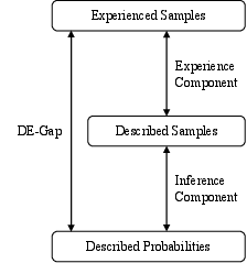
We adopt a conservative replica of the classic DE-Gap experiment (cf. Wulff et al., 2018), yoking a Described-Probabilities treatment to an Experienced-Samples treatment. To disentangle the two DE-Gap components, we add a Described-Samples treatment. The difference between Experienced Samples and Described Samples constitutes the experience component and that between Described Samples and Described Probabilities constitutes the inference component (see Figure 3).
font=footnotesize
| Figure 3: DE-Gap Composition |
We then exploit exogenous variation to test econometrically whether it is statistical confidence that creates an inference component of DE-Gaps. Yoking outcome proportions in Experienced Samples to choice sets in the Described-Samples and Described-Probabilities treatments exogenously varies statistical confidence for these two latter treatments (Rakow et al., 2008,Hau et al., 2010,HertwigPleskac, 2010). Our model thus estimates the probability of subject i in decision choice set j to choose as if underweightingi,j as a function of statistical confidencei,j, experimental treatmenti, and their interaction, controlling for choicesetj, and with errors єi,j clustered at the subject level:
underweighting_i,j = α+ β_1 ·confidence_i,j + β_2 ·treatment_i
+ β_3 ·confidence_i,j ·treatment_i + β_4 ·choiceset_j + є_i,j.
4.2 Experiment 1
Our experiments are computer-based, using the oTree framework (Chen et al., 2016). The first experiment enlisted bachelor and masters students at a European university. 214 students completed the experiment in 9 sessions (65% male, mean age = 20.4 years), a subject number that exceeds the DE-Gap study norm (Wulff et al., 2018). Each subject received 10 points as an initial endowment and additionally played out one randomly selected choice at the end of the experiment. This bonus ranged from −10 to 32 points and averaged 0.1. Compensation was through session-level sweepstakes of €50 conditional on the sum of endowed and additional points (Tollock, 1980), which permits higher-powered incentivization than piece rates for everyone while guarding against the risk-preference skew of ranked winner-takes-all schemes (Connelly et al., 2014,Dechenaux et al., 2015).
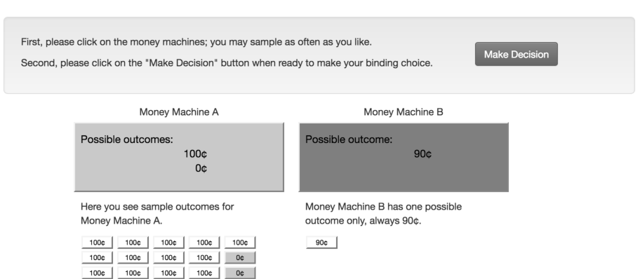
The experiment asked subjects to make ten choices between two money machines each (see Table 2). Each choice pair contains a risky money machine (i.e., one possible high outcome and one possible low outcome, with non-zero probabilities) and a safe money machine (i.e., one certain outcome). Subjects receive information on the possible outcomes of each money machine (for detail on the visual stimuli, see Appendix A).
[b]
[para,flushleft]
Notes. Risky choices render one outcome with probability
p and another with probability 1−
p. Safe choices have one outcome only. Prior Use indicates the number of papers reviewed by
(Wulff et al., 2018) that include the choice set. We compare prior results to our own.
The focal five choice sets are from canonical DE-Gap studies, three from (Hertwig et al., 2004), and two from (BarronErev, 2003). These five are the most frequently studied problems in the DE-Gap articles reviewed by (Wulff et al., 2018). They encompass positive and negative outcomes, small and large in magnitude, as well as expected-value-equivalent and non-equivalent pairs.
We complemented the classic sets with five additional filler choices, which are meant to reduce the chances of subjects approaching decision making with two types of informed priors. First, to avoid the impression that one of the two outcomes of a risky machine is always disproportionately rare, we included two choice sets with equal-probability outcomes (Choice Sets 6 and 7 in Table 2), one in the loss and one in the gain domain. Second, to avoid the impression that the two choices always offer similar payoffs in expectation, we included three choice sets where expected values differ substantially between the two money machines (Choice Sets 8-10 in Table 2). These three choice sets cover both gain and loss, as well as small and large outcomes. We randomized the display sequence of the ten choice sets as well as the left/right placement of the safe and risky machines.
The treatment Experienced Samples encompasses 49 subjects from the first 3 sessions. Subjects choose after sampling as often as they like. In all treatments, money-machine outcomes were stated explicitly — for instance, “4 points or 0 points”, ruling out sample-space unawareness (Smithson et al., 2000,HadarFox, 2009). Sample draws were recorded on the screen to reduce the scope for memory-limitation confounds (e.g., Hertwig et al., 2004,Hau et al., 2008,Rakow et al., 2008,Ungemach et al., 2009).
The frequencies of random sample draws in the Experienced-Samples treatment provide the probabilities in the decision problems for subsequent treatments. Such yoking (Rakow et al., 2008,Hau et al., 2010,HertwigPleskac, 2010) ensures that the proportions seen in the Experienced-Samples treatment are also those that subjects in other treatments see. Yoking rules out sampling error as a mechanical explanation for our DE-Gaps (e.g., FoxHadar, 2006,Hau et al., 2008,Ungemach et al., 2009,Hau et al., 2010) and avoids the side effects of other remedies.7
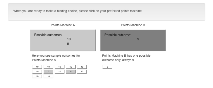
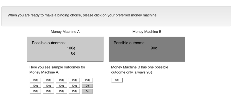
Described Samples encompasses 81 subjects randomly allocated from the latter 6 sessions.8 This treatment mirrors Experienced Samples, except that there is no independent sampling. Instead, subjects are shown the final sample records of their yoked counterparts.9 Subjects are told that these randomly drawn samples were the record of previous plays at each machine (for detail on instructions, see Appendix A).
The difference between Described Samples and Experienced Samples is that subjects in the latter treatment experience the sampling process, whereas subjects in the former merely see the final sample records. Experiencing the sampling process involves drawing samples successively and, in our case, autonomously deciding when to stop sampling.
Our Described-Samples treatment is closest to Condition 3 in the DE-Gap study of (Rakow et al., 2008) and the Yoked-Description condition in (HertwigPleskac, 2010). Both provide subjects with sample summaries. Extending the robustness of these earlier efforts, we keep the visual display of samples constant between sample treatments. We also state the sample space and provide sample records. Together with yoking, these extensions rule out sampling error and amplification, sample-space unawareness, and sample-memory limitations as alternative explanations for the reported findings.
Also related, but with a different premise, is the study of (Smithson et al., 2019) who compared experienced and described samples but did not allow for random sampling. Nor did (CamilleriNewell, 2019), who examined probability judgments and employed money machines that treated sample frequencies as population probabilities (unsuitable for studying choices in contexts where samples only partially reflect populations).
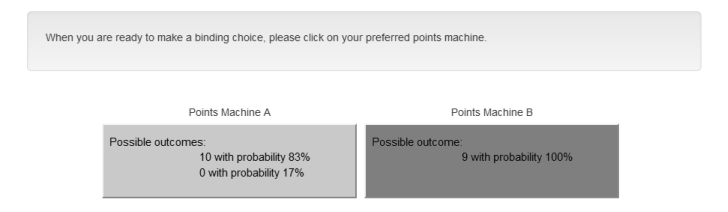
Described Probabilities encompasses 84 subjects randomly allocated from the latter 6 sessions. As in the classic treatment design (Hertwig et al., 2004), subjects were shown yoked probabilities for the outcomes of each money machine — for instance, “4 points with probability 80% or 0 points with probability 20%”.
4.3 Experiment 2
We used Amazon Mechanical Turk (Litman et al., 2017) for replication with a different subject pool and incentivization with piece rates. A total of 299 US-based Amazon Mechanical Turk workers were recruited as subjects (53% male, mean age = 36.8 years). Subjects were asked to make the same ten choices as in Experiment 1. Each subject received an Amazon worker fix-pay of $3 for their participation. In addition, each subject received an initial endowment of $1 for the experiment. As in Experiment 1, one choice set was randomly drawn to determine their additional bonus. All subjects were paid out. The average variable pay was $0.1, ranging from −$1 to $3.2.
Experiment 2 is based on the same design as Experiment 1. One hundred three subjects participated in the Experienced-Samples treatment. Afterward, we again yoked the experienced sample frequencies to the description treatments. Description treatments were run in parallel, randomly assigning 97 subjects to the Described-Probabilities treatment and 99 to the Described-Samples treatment.
4.4 Extant Data
To compare our work with that of prior studies, we retrieved the dataset used for a meta-analysis of DE-Gap research (Wulff et al., 2018). The dataset contains Described-Probabilities and Experienced-Samples treatments only. The data pertain to experiments that share many features of the canonical design such as the autonomous-sampling paradigm. Some designs differ from ours in that they do not display sample records to participants, state the outcome space, or yoke choice parameters across treatments. The (Wulff et al., 2018) dataset contains no information on the yoke pairings when yoking did take place.
5 Analyses
For both our and extant datasets, we restrict analyses to the focal choice sets 1-5 and to meaningful observations in which small probabilities can be underweighted (tests for robustness to exclusions are provided in Appendix D). To permit such underweighting, choices must first involve risk. If Experienced-Samples subjects choose before having drawn both possible outcomes from the risky machine, the yoked choice pair in Described Probabilities contains no risk, asking subjects to choose between two safe machines. These subjects cannot attach weights to probabilities for non-existent events. Free sampling necessarily creates such safe-only choices for almost all participants at least some of the time (Wulff et al., 2018). We exclude all safe-only choices and their yokes from the main analyses.
Underweighting of small probabilities also requires a minimum sample size so that a supposedly rare outcome is in fact rare. Very small sample sizes make drawing a supposedly rare event seem a common occurrence in sample treatments (HertwigPleskac, 2008,HertwigPleskac, 2010) and are guaranteed to be a common occurrence in the yoked Described-Probability treatment. With a sample size of five or larger, supposedly rare events more likely occur in lower proportions. This restriction level is informed by the DE-Gap convention for rare, which is one in five or fewer (Wulff et al., 2018). After exclusions, our main analyses involve 507 Experiment-1 decisions, 529 Experiment-2 decisions, and 4,039 decisions observed in prior work.
5.1 The DE-Gap in Group-Mean Underweighting Choices
Our first finding is that the often-observed gap in probability weighting is partially due to the difference between receiving information through experience and description (the experience component), and partially due to the difference between inferring probabilities from samples and receiving stated probabilities (the inference component). We begin by showing these differences in the proportion of subjects choosing as if they underweight the probability of a rare event. As per Table 2, we code such choices as 1 if subjects
- reject risky options with attractive rare outcomes, and
- select risky options with unattractive rare outcomes (e.g., Hertwig et al., 2004,HertwigErev, 2009),
otherwise 0.
Figure 4 summarizes how a DE-Gap can contain a non-trivial inference component, in addition to an experience component (for detailed results, please see Figure C1 in Appendix C). The inference component constitutes 33% of the overall DE-Gap in our experiments. Figure 4 also compares our data to prior evidence with our choice sets 1-5. The overall DE-Gap magnitudes in our and extant data are comparable, offering an empirical suggestion that previously reported DE-Gaps may not exclusively identify experience effects.
| Figure 4: DE-Gaps in the Treatment Proportions of Underweighting Choices |
To inspect the robustness of comparisons between our and extant data, we randomly select 100 observations from each treatment and dataset, a thousand times (see Figure C2 in Appendix C for detail). The distribution of the 1000 DE-Gaps are closely aligned for both datasets. Comparability thus is not an accident and the systematic gap structure displayed in Figure 4 likely reliable.
Note that in our specification, the inference component is positive, but, as Section 3 illustrates, studies with different choice sets and sample patterns could generate a negative inference component too. So rather than making a claim about the general form of DE-Gaps’ inference component, we here merely show that non-negligible magnitudes of this component exist, potentially confounding experience effects in previously observed DE-Gaps.
Another way to interpret the choice data is to compare the underweighting likelihood of subjects in the Experienced-Samples treatment with that of subjects in the other treatments (see Table 3). The odds for Experienced-Sample subjects are significantly larger than those for Described-Probabilities subjects but not necessarily those for Described-Samples subjects. In our two experiments, the experience-only component of the overall DE-Gap difference in odds is small enough to be insignificant at a 95% level. We further probe these results with a parameter estimation in the following section.
| Table 3: Relative Likelihood of Underweighting Choices |
| Experienced Samples | vs Described Probabilities | vs Described Samples |
|
| 20.4@percentExperiments 1+2 (this paper) | 1.58 | 1.36 |
| | [1.10-2.26] | [0.96-1.95] |
| 20.4@percent16 Experiments (Wulff et al. 2018) | 1.59 | n.a. |
| | [1.38-1.85] | n.a. |
|
[para, flushleft]
Notes. The table contains the odds for subjects in the Experienced-Samples treatment to choose as if they underweight small probabilities, relative to subjects in the indicated baseline treatments. 95% confidence intervals (CI) in brackets. Values pertain to the β1 parameter from logistic regressions of the form:
underweightingi,j = α + β1 · treatment + β2 · choiceset + β3 · experiment + єi,
where i and j are decision and subject indices, respectively.
5.2 The DE-Gap in Estimated Probability-Weights
The preceding analyses of proportions and odds are straightforward but require researchers to categorize choices as underweighting. Alternatively, one can estimate probability weights on the basis of observed choice behavior. We thus follow established practice (Abdellaoui et al., 2011,Wulff et al., 2018,Hotaling et al., 2019) and complement our analyses with a decision parameter estimation that builds on cumulative prospect theory (CPT, (TverskyKahneman, 1992)).10
Since CPT estimations require no particular problem structure for the identification of underweighting, we can include choice sets 6-10 as well, thus enhancing reliability in the mid range of probability. For extant data, we additionally include all classical choice sets where one risky outcome is zero. We retain our inclusion criteria of one risky outcome rare and sample size of five or greater, because relaxing them would
- swamp the estimation with probabilities 0 and 1, and
- increase the challenge of comparing unyoked treatments in extant data.
The CPT analyses reported here are, therefore, based on 2,178 Experiment 1 and 2 decisions, and 7,658 decisions from extant work. For transparency, the tables in Appendix D also document estimation parameters for Experiments 1 and 2 when all observations are included. Table 9 in (Wulff et al., 2018) reports the same for extant work.
Our focus is on the CPT parameter γ, which weights p, the described probability or frequency of sample outcomes (Glöckner et al., 2016,Lejarraga et al., 2016). The weighting is determined by function w(p), as proposed by (TverskyKahneman, 1992)11:
w(p)=p^γ/(p^γ + (1- p)^γ)^1/γ .
For γ > 1, the weighting function is S-shaped and suggests underweighting of small probabilities (e.g., CamererHo, 1994,GonzalezWu, 1999,Fehr-DudaEpper, 2011). Conversely, γ < 1 indicates overweighting of small probabilities.
We summarize estimation results for γ in Figure 5 and Table 4 (see Appendix D for a complete list of estimates). In both our and extant data, participants in Described-Probabilities treatments overweight small probabilities, while those in Experienced-Samples treatments underweight. The γ estimates are in line with those reported elsewhere (e.g., Ungemach et al., 2009,Abdellaoui et al., 2011,CamilleriNewell, 2011b,Frey et al., 2015,Glöckner et al., 2016,Kellen et al., 2016,Lejarraga et al., 2016). As per our expectation, the probability weights of participants in the Described-Samples treatments lie between those of their counterparts in the Described-Probabilities and Experienced-Samples treatments. This corroborates our earlier finding that overall DE-Gaps likely consist of both an inference and an experience component.
| Figure 5: Probability Weighting. The graphs display the estimated probability weights w(p) of Equation wTK for each treatment. p is either the described probability or the frequency of sample outcomes. |
| Table 4: DE-Gaps in the Probability-Weighting Parameter γ |
| | | Described Probabilities | Described Samples | Experienced Samples |
| Experiments 1+2 Data | | 0.78 | 0.94 | 1.22 |
| | | [0.63-1.13] | [0.75-1.34] | [0.97-1.64] |
| Data in (Wulff et al., 2018) | | 0.74 | n.a. | 1.04 |
| | | [0.63-0.84] | n.a. | [0.94-1.14] |
|
Notes. The table contains the median γ parameters estimated by the CPT model detailed in Appendix D and used in Figure 5. 95% confidence intervals in brackets.
|
5.3 The Effect of Statistical Confidence
When our decision problems in the Described-Probabilities treatment offer statistical confidence of 0 that the underweighting choice is superior to the alternative, decision problems in the sample treatments offer 0.18 on average. When the Described-Probability treatment offers statistical confidence of 1, the sample treatments offer 0.59 on average. Sample-treatment confidence levels thus depart from those in the Described-Probabilities treatment, rendering qualitatively different decision problems (see Figure 6) even when sampling error and amplification are absent.
| Figure 6: Statistical-Confidence Distributions. The graphs display the estimated probability weights w(p) of Equation wTK for each treatment. p is either the described probability or the frequency of sample outcomes. |
Our yoked design yields smaller departures than prior work does with choice sets 1-5 (extant data from Wulff et al., 2018). Prior work’s sample treatments offer average confidence levels of 0.23 and 0.42, respectively. Unyoked settings are subject to sampling error and amplification that explain the larger differences in the values of statistical confidence across treatments in the extant data.
Underweighting behavior then systematically varies with statistical confidence12, as illustrated in Figure 7. Three observations emerge. First, the probability of a sample decision maker opting for the choice indicating underweighting of small probabilities increases with statistical confidence in the choice. This sensitivity is reassuringly consistent with those documented in studies of decision making under uncertainty (EinhornHogarth, 1985,GigliottiSopher, 1996,ErtTrautmann, 2014,Kutzner et al., 2017).
| Figure 7: Statistical Confidence and Underweighting: |
ES: Experienced Samples
DS: Described Samples
DP: Described Probabilities |
Second, sample decision makers behave as if they underweight more (less) often than population decision makers when sample confidence markedly exceeds (falls short of) population confidence. If population confidence in the superiority of the underweighting choice is 0, for example, and sample confidence 0.3, then sample decision makers will choose as if they underweight more often than population decision makers.
Third, sample decision makers behave as if they underweight less (more) often than population decision makers when sample confidence barely exceeds (falls short of) population confidence. If population confidence in the superiority of the underweighting choice is 0, for example, and sample confidence 0.1, then sample decision makers will choose as if they underweight less often than population decision makers.
These three findings together demonstrate sensitivity to statistical confidence, especially for sample decisions. When sample confidence is less extreme than population confidence, sample decisions are less unequivocal. When sample confidence is almost as extreme as population confidence, sample decision makers’ choices are more resolute by comparison. Sample decision makers more often maximize payoffs as a result. These findings mean that the inference component of DE-Gaps could be positive as well as negative, depending on where average confidence values lie in sample treatments.13
To provide a multivariate econometric test, we estimate a logistic model of as-if-underweighting choices (see Equation conffunction and Table 5). The model predicts individual decisions, addressing potential concerns about behavioral conclusions from group-level analysis (RegenwetterRobinson, 2017,HertwigPleskac, 2018). For better interpretation, we additionally plot the marginal effects of statistical confidence in Figure 8.
| Table 5: Logit Estimation of Underweighting |
| | Experiments 1 & 2, Yoked | | 16 Experiments in Prior Studies, Unyoked |
| | | | Data by (Wulff et al., 2018) |
|
|
|
Predictors | Coefficient | z-statistic | p value | 95% CI | | Coefficient | z-statistic | p value | 95% CI |
|
|
Described Samples (DS) | −0.40 | −1.44 | .150 | [−0.94,0.14] | | - | - | - | - |
| Experienced Samples (ES) | −0.57 | −1.77 | .078 | [−1.21,0.06] | | −0.34 | −2.07 | .039 | [−0.66, −0.02] |
| Statistical Confidence | 0.95 | 3.67 | .000 | [0.44,1.46] | | −0.05 | −0.28 | .777 | [−0.42, 0.32] |
| Statistical Confidence × DS | 1.69 | 3.05 | .002 | [0.60, 2.78] | | - | - | - | - |
| Statistical Confidence × ES | 3.17 | 3.90 | .000 | [1.58, 4.76] | | 2.07 | 7.70 | .000 | [1.54, 2.59] |
| Intercept | −1.00 | −3.93 | .000 | [−1.50, −0.50] | | −0.70 | −2.91 | .004 | [−1.17, −0.23] |
| Choice-Set Dummies | yes | | yes |
| Experiment Dummies | yes | | yes |
| Number of Decisions | 1,036 | | 4,039 |
| Log Likelihood | −655.01 | | −2576.59 |
| χ2 | 81.86 | | 314.56 |
| Pseudo R2 | 0.09 | | 0.07 |
|
[para,flushleft]
Notes.
The table contains logistic-regression coefficients for subjects choosing the underweighting choice. Analysis is at the decision level, with errors clustered at the subject level. The baseline are decisions based on described probabilities.
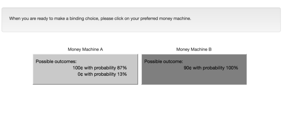
Figure 8: Margin Plots.
The graphs plot the marginal effects of the table models.
The (Wulff et al., 2018) dataset contains no Described-Samples treatment. The Described-Probabilities and Experienced/Samples treatments are also not yoked: described probabilities are fixed and do not correspond to sample proportions. The Described-Probabilities treatments in the (Wulff et al., 2018) data, therefore, always involve an underweighting choice and an alternative that are almost equivalent in expected value, whereas experience-treatment decisions involve choices with amplified expected-value differences (HertwigPleskac, 2010). In our yoked experiment designs, by contrast, the difference in expected value between the two choices co-varies across treatments. The effect of confidence in our data can, therefore, be directly compared with the (Wulff et al., 2018) data for the Experienced-Samples treatment only. |
The logistic models confirm trends visible in the raw data of Figure 7. The likelihood of choosing as if underweighting significantly increases with statistical confidence. With statistical confidence being accounted for in the logistic models of Table 5, the coefficients for the experimental-treatment dummies are of low significance. The interactions of statistical confidence and treatment dummies, by contrast, explain more variance. Treatment membership appears to alter the slope of the confidence effect. Decisions in Experienced Samples and Described Samples are more responsive to levels of statistical confidence than Described Probabilities. Sensitivity to statistical confidence in sample treatments compares (the 95% intervals in Figure 8 overlap), even though statistical confidence is exogenously determined in the Described-Samples treatment only, and partly endogenously determined in the Experienced-Samples treatment. The results for a confidence effect in sample treatments are consistent across our experiments as well as those reviewed by (Wulff et al., 2018). In prior work, reported DE-Gaps appear to stem from differences in statistical confidence across treatments.
In conclusion, our study shows that the DE-Gap reported in prior studies has an inference component. This inference component could be positive as well as negative. Risky decisions are sensitive to statistical confidence levels, irrespective of whether decision makers experienced sample draws or saw a description of them.
6 Discussion
In this paper, we offer a novel explanation for frequently observed description-experience gaps. Replicating the original gap in a yoked design, we show that part of the gap is due to the difference in the statistical properties of the decision problems in experimental treatments. Decisions based on samples are sensitive to statistical confidence. Underweighting behavior thus departs from that in decisions based on population probabilities (the inference component of DE-Gaps). When the same samples are described and when they are experienced, choice behavior remains distinct (the experience component of DE-Gaps).
6.1 The Inference Component of DE-Gaps
Our study shows that the weighting of small probabilities in risky choice based on sample information (such as provided by the typical experience treatment) differs from that in risky choice based on population information (such as provided by the typical description treatment). The difference is systematically related to the level of statistical confidence provided by the sample. This finding is consistent with studies of decision making under uncertainty (e.g., EinhornHogarth, 1985,Kutzner et al., 2017) and provides an explanation for why prior studies found smaller DE-Gaps when experience and description treatments likely offered similar levels of statistical confidence. For example, smaller gaps were reported when experience decisions were based on forcibly large samples (Jarvstad et al., 2013) and exhaustive samples (HilbigGlöckner, 2011,AydoganGao, 2020,Cubitt et al., 2022). When samples are forcibly large or exhaustive, statistical confidence levels in sample and population decisions converge toward 0 or 1. In studies with smaller samples, statistical conditions are comparable only if description is also with samples.14
Previously reported description-experience gaps thus likely contain an inference component, and variation in statistical confidence appears to explain it. Our identification is facilitated by the experimental design’s robustness to sampling error; we strictly yoke all our experimental treatments. We also rule out cognitive constraints by providing sample records and stating sample spaces. In the absence of statistical and cognitive confounds, we reveal how exogenously determined statistical confidence in sample decisions drives decision makers’ revealed preference for underweighting choices.
The econometric analysis confirms our expectation that sample decision makers show moderate underweighting behavior at intermediate values of statistical confidence — values that are offered by sample evidence only. Underweighting at intermediate values of confidence ranges between the underweighting observed for the two extreme values of 0 and 1 — values that are offered by fully specified probabilities only. Intriguingly, however, our findings also show that relative underweighting differences reverse in the vicinity of extreme statistical confidence. For example, decisions based on samples more often involve as-if-underweighting choices that are very likely superior in expectation, than decisions do that are based on population information offering surety. What at first may look like more underweighting actually is more reasonable choice behavior. It suggests that decisions based on samples from an unknown probability distribution more often follow those of a risk-neutral Bayesian than decisions based on descriptions of known probabilities.
Consistent with this finding, a recent study by (CamilleriNewell, 2019) in the DE-Gap realm reports that probability judgments match outcome distributions more often when sample information is sequentially received than when it is summarily received. The authors ascribe the better calibration, in their case reduced over-precision, to learning through experience, rather than description. Their argument is that experiential learning makes for better recall of distributions than learning from description. Subjects learning from description expect more extreme outcomes than subjects learning from experience, arguably because description does not allow for the repeated prediction, prediction-error, and prediction-adjustment cycles of experience.
While this recall effect may explain why sensitivity to statistical confidence is somewhat larger for our Experienced-Samples subjects than for our Described-Samples subjects, it cannot explain why sample decisions are more sensitive to statistical confidence than population decisions. ((CamilleriNewell, 2019) do not have a treatment on described probabilities for populations.) Descriptions of fully specified probabilities for a known outcome space preclude the existence of further or more frequent extreme outcomes and require no inference.
The inference gap between decisions based on sample and population information may stem from the more intuitive processing of natural frequencies (GigerenzerHoffrage, 1995). Although sample records require inference that fully specified probabilities do not, the exercise may lead people to make better decisions in expectation. Estimations based on sample evidence are noisy (Olschewski et al., 2021), but the cognitive process alone might help people make more calibrated decisions. They might think through choice alternatives in a way that more naturally matches everyday cognitive demands than the way population statistics require. (NewellRakow, 2007) provide some indication of this: subjects made better decisions when sample outcomes were provided alongside fully-stated probabilities than when relying on the description only.
Decision makers seeing population statistics, on the other hand, appear to try to mentally simulate the distribution of outcomes described in population statistics (Erev et al., 2017,Weiss-Cohen et al., 2018). They might not always be willing to undertake this cognitive effort and thus arrive at suboptimal choices than sample decision makers, who are naturally led to infer.
Future research on the cognitive role of statistical confidence may thus shed light on decision-making behavior ostensibly at odds with classic notions of revealed preferences. The formation of beliefs about underlying probabilities appears to explain behavior under uncertainty (ErtTrautmann, 2014,Baillon et al., 2017,Aydogan, 2021,Cubitt et al., 2022), and our work points to subjective inferences being more consistent with statistical confidence in sample contexts.
6.2 The Experience Component of DE-Gaps
Our research design isolates the inference component from DE-Gaps and thus permits more direct examination of causes for the experience component. Our data contains perceptible differences in choice behavior between decisions based on experienced samples and those based on described samples.
Our finding complements (Rakow et al., 2008), who report little difference in choice behavior between experienced and described samples. One take-away from both (Rakow et al., 2008) and our stricter version is that comparing described and experienced samples permits examination of experience that is robust to confounding variation in information across treatments. It allows future research to be more precise about what it might mean for people to be “living through events” (Hertwig et al., 2018, p.2) rather than just to read about them (see also HertwigWulff, 2020). To that end, our econometric analyses suggest experience has a moderating effect on sensitivity to statistical confidence.
Experience makes sampling cost salient, both economic, in terms of the time required for amassing evidence, and affective, in terms of the emotions of uncovering positive and negative evidence (Konstantinidis et al., 2018). Being in control of sampling, including when (not) to stop, may additionally influence how comfortable decision makers feel with risky choices. These may be directions for future inquiry aided by the more precise identification of experience components that we contribute.
More obvious perhaps is that people who iteratively sample may be subject to primacy, order, and recency effects in a way that people receiving sample descriptions cannot be. Particular sample-draw patterns might influence beliefs more strongly than others, even when samples are recorded. Our experiments were not designed to identify such sequencing effects. But it is conceivable that the sequential revelation of sample evidence makes people repeatedly test and update their probability projections and, therefore, make better decisions than people who decide on the basis of a sample record (Hohwy, 2013,CamilleriNewell, 2019). An extension to instance-based learning theory (Gonzalez et al., 2003,Lejarraga et al., 2012) might perhaps be able to account for such mechanisms, offering a means to examine description-experience gaps in decisions based on samples.
6.3 Implications for Decision Making
In contrast to popular experimental stimuli in decision science, people are rarely afforded fully specified probabilities when they make risky choices. No amount of experimentation or due diligence can offer fully specified probabilities of new-product failure and success, for example. Instead, people must rely on sample observations, provided by their own experience or through description of others’ experiences. So, when people choose between competing alternatives, their choice behavior more likely follows that observed in decisions based on samples than in decisions based on fully specified probabilities.
Our work reveals that the likely greater underweighting in organizational choice contexts need not be a bias. Experiencing sample evidence, such as the developer of a new product might (FeilerTong, 2021), may distort decisions through primacy, order, recency, or other sequencing effects. However, uninvolved decision-makers who merely see descriptions of sample evidence are not subject to such experience biases. Think executives who review record of a new-product development project, for example (KlingebielRammer, 2021). These decision makers’ underweighting behavior might then be an indication of statistical reasoning. Their debiasing might be further enhanced by ensuring appropriate priors (Farmer et al., 2017) and stimulating inference through visualizations of probability distributions (Kaufmann et al., 2013,GoldsteinRothschild, 2014). Our study thus opens up avenues for further research on improving real-world decision making.
7 Conclusion
Real-world decisions are often, but not always, based on experience, and virtually always based on limited sample evidence. Our work adds to the understanding of how each might contribute to frequently observed DE-Gaps. In particular, we show that sensitivity to statistical confidence leads to probability weighting in decisions based on samples that differ from decisions based on stated probabilities. Sample decision makers behave as if they underweight more than decision makers who need not infer probabilities. Yet, their choices more often maximize payoffs than the choices of those who receive fully specified probabilities. Real-world decision makers could turn out less biased than research based on fully described population probabilities might suggest.
References
-
[Abdellaoui et al., 2011]
-
Abdellaoui, M., L’Haridon, O., & Paraschiv, C. (2011).
Experienced vs. described uncertainty: Do we need two prospect theory
specifications?
Management Science, 57(10), 1879–1895.
- [Andersen et al., 2010]
-
Andersen, S., Harrison, G. W., Lau, M. I., & Rutström, E. E. (2010).
Behavioral econometrics for psychologists.
Journal of Economic Psychology, 31(4), 553–576.
- [Ashby et al., 2017]
-
Ashby, N. J., Konstantinidis, E., & Yechiam, E. (2017).
Choice in experiential learning: True preferences or experimental
artifacts?
Acta Psychologica, 174, 59–67.
- [Aydogan, 2021]
-
Aydogan, I. (2021).
Prior beliefs and ambiguity attitudes in decision from experience.
Management Science, 67(11), 6934–6945.
- [AydoganGao, 2020]
-
Aydogan, I. & Gao, Y. (2020).
Experience and rationality under risk: Re-examining the impact of
sampling experience.
Experimental Economics, 23, 1100–1128.
- [Baillon et al., 2017]
-
Baillon, A., Bleichrodt, H., Keskin, U., L’Haridon, O., & Li, C. (2017).
The effect of learning on ambiguity attitudes.
Management Science, 64(5), 2181–2198.
- [BarronErev, 2003]
-
Barron, G. & Erev, I. (2003).
Small feedback-based decisions and their limited correspondence to
description-based decisions.
Journal of Behavioral Decision Making, 16(3), 215–233.
- [BarronYechiam, 2009]
-
Barron, G. & Yechiam, E. (2009).
The coexistence of overestimation and underweighting of rare events
and the contingent recency effect.
Judgment and Decision Making, 4(6), 447–460.
- [Bayes et al., 1763]
-
Bayes, T., Price, R., & Canton, J. (1763).
An essay towards solving a problem in the doctrine of chances.
Philosophical Transactions of the Royal Society of London, 53, 370–418.
- [BazermanMoore, 2013]
-
Bazerman, M. H. & Moore, D. A. (2013).
Judgment in Managerial Decision Making.
Hoboken, New Jersey: John Wiley & Sons.
- [BernardoSmith, 1994]
-
Bernardo, J. M. & Smith, A. F. M. (1994).
Bayesian Theory.
Chichester: John Wiley & Sons.
- [BolstadCurran, 2016]
-
Bolstad, W. M. & Curran, J. M. (2016).
Introduction to Bayesian Statistics.
Hoboken, New Jersey: John Wiley & Sons.
- [Brown et al., 2001]
-
Brown, L. D., Cai, T. T., & DasGupta, A. (2001).
Interval estimation for a binomial proportion.
Statistical Science, 16(2), 101–133.
- [CamererHo, 1994]
-
Camerer, C. F. & Ho, T. H. (1994).
Violations of the betweenness axiom and nonlinearity in probability.
Journal of Risk and Uncertainty, 8(2), 167–196.
- [CamilleriNewell, 2011a]
-
Camilleri, A. R. & Newell, B. R. (2011a).
Description- and experience-based choice: Does equivalent information
equal equivalent choice?
Acta Psychologica, 136(3), 276–284.
- [CamilleriNewell, 2011b]
-
Camilleri, A. R. & Newell, B. R. (2011b).
When and why rare events are underweighted: A direct comparison of
the sampling, partial feedback, full feedback and description choice
paradigms.
Psychonomic Bulletin & Review, 18(2), 377–384.
- [CamilleriNewell, 2019]
-
Camilleri, A. R. & Newell, B. R. (2019).
Better calibration when predicting from experience (rather than
description).
Organizational Behavior and Human Decision Processes, 150, 62–82.
- [Chen et al., 2016]
-
Chen, D. L., Schonger, M., & Wickens, C. (2016).
oTree – An open-source platform for laboratory, online, and
field experiments.
Journal of Behavioral and Experimental Finance, 9(2),
88–97.
- [Connelly et al., 2014]
-
Connelly, B. L., Tihanyi, L., Crook, T. R., & Gangloff, K. A. (2014).
Tournament theory: Thirty years of contests and competitions.
Journal of Management, 40(1), 16–47.
- [Cubitt et al., 2022]
-
Cubitt, R. P., Kopsacheilis, O., & Starmer, C. (2022).
An inquiry into the nature and causes of the Description-Experience
gap.
Journal of Risk and Uncertainty.
Forthcoming.
- [de Palma et al., 2014]
-
de Palma, A., et al. (2014).
Beware of black swans: Taking stock of the description–experience
gap in decision under uncertainty.
Marketing Letters, 25(3), 269–280.
- [Dechenaux et al., 2015]
-
Dechenaux, E., Kovenock, D., & Sheremeta, R. M. (2015).
A survey of experimental research on contests, all-pay auctions and
tournaments.
Experimental Economics, 18(4), 609–669.
- [EinhornHogarth, 1985]
-
Einhorn, H. J. & Hogarth, R. M. (1985).
Ambiguity and uncertainty in probabilistic inference.
Psychological Review, 92(4), 433–461.
- [Erev et al., 2017]
-
Erev, I., Ert, E., Plonsky, O., Cohen, D., & Cohen, O. (2017).
From anomalies to forecasts: Toward a descriptive model of decisions
under risk, under ambiguity, and from experience.
Psychological Review, 124(4), 369–409.
- [Erev et al., 2008]
-
Erev, I., Glozman, I., & Hertwig, R. (2008).
What impacts the impact of rare events.
Journal of Risk and Uncertainty, 36(2), 153–177.
- [ErtTrautmann, 2014]
-
Ert, E. & Trautmann, S. T. (2014).
Sampling experience reverses preferences for ambiguity.
Journal of Risk and Uncertainty, 49(1), 31–42.
- [Farmer et al., 2017]
-
Farmer, G. D., Warren, P. A., & Hahn, U. (2017).
Who “believes” in the Gambler’s Fallacy and why?
Journal of Experimental Psychology: General, 146(1),
63–76.
- [Fehr-DudaEpper, 2011]
-
Fehr-Duda, H. & Epper, T. (2011).
Probability and risk: Foundations and economic implications of
probability-dependent risk preferences.
Annual Review of Economics, 4, 567–593.
- [FeilerTong, 2021]
-
Feiler, D. & Tong, J. (2021).
From Noise to Bias: Overconfidence in New Product Forecasting.
Management Science.
Advance online publication. Available at
https://doi.org/10.1287/mnsc.2021.4102.
- [FoxHadar, 2006]
-
Fox, C. R. & Hadar, L. (2006).
Decisions from experience = sampling error + prospect theory:
Reconsidering Hertwig, Barron, Weber & Erev (2004).
Judgment and Decision Making, 1(2), 159–161.
- [Frey et al., 2015]
-
Frey, R., Mata, R., & Hertwig, R. (2015).
The role of cognitive abilities in decisions from experience: Age
differences emerge as a function of choice set size.
Cognition, 142, 60–80.
- [GigerenzerHoffrage, 1995]
-
Gigerenzer, G. & Hoffrage, U. (1995).
How to improve Bayesian reasoning without instruction: Frequency
formats.
Psychological Review, 102(4), 684–704.
- [GigliottiSopher, 1996]
-
Gigliotti, G. & Sopher, B. (1996).
The testing principle: Inductive reasoning and the Ellsberg
paradox.
Thinking & Reasoning, 2(1), 33–49.
- [Glöckner et al., 2016]
-
Glöckner, A., Hilbig, B. E., Henninger, F., & Fiedler, S. (2016).
The reversed description-experience gap: Disentangling sources of
presentation format effects in risky choice.
Journal of Experimental Psychology: General, 145(4),
486–508.
- [GoldsteinRothschild, 2014]
-
Goldstein, D. G. & Rothschild, D. (2014).
Lay understanding of probability distributions.
Judgment and Decision Making, 9(1), 1–14.
- [Gonzalez et al., 2003]
-
Gonzalez, C., Lerch, J. F., & Lebiere, C. (2003).
Instance-based learning in dynamic decision making.
Cognitive Science, 27(4), 591–635.
- [GonzalezWu, 1999]
-
Gonzalez, R. & Wu, G. (1999).
On the shape of the probability weighting function.
Cognitive Psychology, 38(1), 129–166.
- [Gottlieb et al., 2007]
-
Gottlieb, D. A., Weiss, T., & Chapman, G. B. (2007).
The format in which uncertainty information is presented affects
decision biases.
Psychological Science, 18(3), 240–246.
- [GriffinTversky, 1992]
-
Griffin, D. & Tversky, A. (1992).
The weighing of evidence and the determinants of confidence.
Cognitive Psychology, 24(3), 411–435.
- [HadarFox, 2009]
-
Hadar, L. & Fox, C. R. (2009).
Information asymmetry in decision from description versus decision
from experience.
Judgment and Decision Making, 4(4), 317–325.
- [Harrison, 2008]
-
Harrison, G. W. (2008).
Maximum likelihood estimation of utility functions using Stata.
Working paper, University of Central Florida.
- [HarrisonRutström, 2008]
-
Harrison, G. W. & Rutström, E. E. (2008).
Risk aversion in the laboratory.
In J. Cox & G. W. Harrison (Eds.), Risk Aversion in
Experiments (Research in Experimental Economics, Vol. 12) (pp.
41–196). Bingley: Emerald Group Publishing Limited.
- [Hau et al., 2010]
-
Hau, R., Pleskac, T. J., & Hertwig, R. (2010).
Decisions from experience and statistical probabilities: Why they
trigger different choices than a priori probabilities.
Journal of Behavioral Decision Making, 23(1), 48–68.
- [Hau et al., 2008]
-
Hau, R., Pleskac, T. J., Kiefer, J., & Hertwig, R. (2008).
The description–experience gap in risky choice: The role of sample
size and experienced probabilities.
Journal of Behavioral Decision Making, 21(5), 493–518.
- [HeDai, 2022]
-
He, Z. & Dai, J. (2022).
Context-dependent outcome expectation contributes to experience-based
risky choice.
Judgment & Decision Making, 17(1).
- [Hertwig et al., 2004]
-
Hertwig, R., Barron, G., Weber, E. U., & Erev, I. (2004).
Decisions from experience and the effect of rare events in risky
choice.
Psychological Science, 15(8), 534–539.
- [HertwigErev, 2009]
-
Hertwig, R. & Erev, I. (2009).
The description–experience gap in risky choice.
Trends in Cognitive Sciences, 13(12), 517–523.
- [Hertwig et al., 2018]
-
Hertwig, R., Hogarth, R. M., & Lejarraga, T. (2018).
Experience and description: Exploring two paths to knowledge.
Current Directions in Psychological Science, 27(2),
123–128.
- [HertwigPleskac, 2008]
-
Hertwig, R. & Pleskac, T. J. (2008).
The game of life: How small samples render choice simpler.
In N. Chater & M. Oaksford (Eds.), The Probabilistic Mind:
Prospects for Bayesian Cognitive Science (pp. 209–235). Oxford:
Oxford University Press.
- [HertwigPleskac, 2010]
-
Hertwig, R. & Pleskac, T. J. (2010).
Decisions from experience: Why small samples?
Cognition, 115(2), 225–237.
- [HertwigPleskac, 2018]
-
Hertwig, R. & Pleskac, T. J. (2018).
The construct–behavior gap and the description–experience gap:
Comment on Regenwetter and Robinson (2017).
Psychological Review, 125(5), 844–849.
- [HertwigWulff, 2020]
-
Hertwig, R. & Wulff, D. U. (2020).
A description–experience framework of the dynamic response to risk.
https://doi.org/10.31234/osf.io/qrph5.
- [HilbigGlöckner, 2011]
-
Hilbig, B. E. & Glöckner, A. (2011).
Yes, they can! Appropriate weighting of small probabilities as a
function of information acquisition.
Acta Psychologica, 138(3), 390–396.
- [Hill, 1968]
-
Hill, B. M. (1968).
Posterior distribution of percentiles: Bayes’ theorem for sampling
from a population.
Journal of the American Statistical Association, 63(322),
677–691.
- [HogarthEinhorn, 1992]
-
Hogarth, R. M. & Einhorn, H. J. (1992).
Order effects in belief updating: The belief-adjustment model.
Cognitive Psychology, 24(1), 1–55.
- [Hohwy, 2013]
-
Hohwy, J. (2013).
The Predictive Mind.
Oxford: Oxford University Press.
- [Hotaling et al., 2019]
-
Hotaling, J. M., Jarvstad, A., Donkin, C., & Newell, B. R. (2019).
How to change the weight of rare events in decisions from experience.
Psychological Science, 30(12), 1767–1779.
- [Jarvstad et al., 2013]
-
Jarvstad, A., Hahn, U., Rushton, S. K., & Warren, P. A. (2013).
Perceptuo-motor, cognitive, and description-based decision-making
seem equally good.
Proceedings of the National Academy of Sciences of the United
States of America, 110(40), 16271–16276.
- [Jessup et al., 2008]
-
Jessup, R. K., Bishara, A. J., & Busemeyer, J. R. (2008).
Feedback produces divergence from prospect theory in descriptive
choice.
Psychological Science, 19(10), 1015–1022.
- [KahnemanTversky, 1979]
-
Kahneman, D. & Tversky, A. (1979).
Prospect theory: An analysis of decision under risk.
Econometrica, 47(2), 263–291.
- [Karmarkar, 1979]
-
Karmarkar, U. S. (1979).
Subjectively weighted utility and the Allais paradox.
Organizational Behavior and Human Performance, 24(1),
67–72.
- [Kaufmann et al., 2013]
-
Kaufmann, C., Weber, M., & Haisley, E. (2013).
The role of experience sampling and graphical displays on one’s
investment risk appetite.
Management Science, 59(2), 323–340.
- [Kellen et al., 2016]
-
Kellen, D., Pachur, T., & Hertwig, R. (2016).
How (in)variant are subjective representations of described and
experienced risk and rewards?
Cognition, 157, 126–138.
- [KlingebielRammer, 2021]
-
Klingebiel, R. & Rammer, C. (2021).
Optionality and selectiveness in innovation.
Academy of Management Discoveries, 7(3), 328–342.
- [Konstantinidis et al., 2018]
-
Konstantinidis, E., Taylor, R. T., & Newell, B. R. (2018).
Magnitude and incentives: Revisiting the overweighting of extreme
events in risky decisions from experience.
Psychonomic Bulletin & Review, 25, 1925–1933.
- [Kopsacheilis, 2018]
-
Kopsacheilis, O. (2018).
The role of information search and its influence on risk preferences.
Theory and Decision, 84(3), 311–339.
- [Kutzner et al., 2017]
-
Kutzner, F. L., Read, D., Stewart, N., & Brown, G. (2017).
Choosing the devil you don’t know: Evidence for limited sensitivity
to sample size-based uncertainty when it offers an advantage.
Management Science, 63(5), 1519–1528.
- [Laplace, 1986]
-
Laplace, P. S. (1986).
Memoir on the probability of the causes of events.
Statistical Science, 1(3), 364–378.
- [Lejarraga et al., 2012]
-
Lejarraga, T., Dutt, V., & Gonzalez, C. (2012).
Instance-based learning: A general model of repeated binary choice.
Journal of Behavioral Decision Making, 25(2), 143–153.
- [LejarragaLejarraga, 2020]
-
Lejarraga, T. & Lejarraga, J. (2020).
Confidence and the description–experience distinction.
Organizational Behavior and Human Decision Processes, 161, 201–212.
- [Lejarraga et al., 2016]
-
Lejarraga, T., Pachur, T., Frey, R., & Hertwig, R. (2016).
Decisions from experience: From monetary to medical gambles.
Journal of Behavioral Decision Making, 29(1), 67–77.
- [Litman et al., 2017]
-
Litman, L., Robinson, J., & Abberbock, T. (2017).
TurkPrime.com: A versatile crowdsourcing data acquisition platform
for the behavioral sciences.
Behavior Research Methods, 49(2), 433–442.
- [Luce, 1959]
-
Luce, R. D. (1959).
Individual Choice Behavior: A Theoretical Analysis.
New York: John Wiley & Sons.
- [Madan et al., 2014]
-
Madan, C. R., Ludvig, E. A., & Spetch, M. L. (2014).
Remembering the best and worst of times: Memories for extreme
outcomes bias risky decisions.
Psychonomic Bulletin & Review, 21(3), 629–636.
- [NewellRakow, 2007]
-
Newell, B. R. & Rakow, T. (2007).
The role of experience in decisions from description.
Psychonomic Bulletin & Review, 14(6), 1133–1139.
- [Nilsson et al., 2011]
-
Nilsson, H., Rieskamp, J., & Wagenmakers, E.-J. (2011).
Hierarchical Bayesian parameter estimation for cumulative prospect
theory.
Journal of Mathematical Psychology, 55(1), 84–93.
- [Olschewski et al., 2021]
-
Olschewski, S., Newell, B. R., Oberholzer, Y., & Scheibehenne, B. (2021).
Valuation and estimation from experience.
Journal of Behavioral Decision Making.
Advance online publication. Available at
https://doi.org/10.1002/bdm.2241.
- [Ostwald et al., 2015]
-
Ostwald, D., Starke, L., & Hertwig, R. (2015).
A normative inference approach for optimal sample sizes in decisions
from experience.
Frontiers in Psychology, 6.
- [PiresAmado, 2008]
-
Pires, A. M. & Amado, C. (2008).
Interval estimators for a binomial proportion: Comparison of twenty
methods.
REVSTAT – Statistical Journal, 6(2), 165–197.
- [Rakow et al., 2008]
-
Rakow, T., Demes, K. A., & Newell, B. R. (2008).
Biased samples not mode of presentation: Re-examining the apparent
underweighting of rare events in experience-based choice.
Organizational Behavior and Human Decision Processes, 106, 168–179.
- [Rakow et al., 2010]
-
Rakow, T., Newell, B. R., & Zougkou, K. (2010).
The role of working memory in information acquisition and decision
making: Lessons from the binary prediction task.
Quarterly Journal of Experimental Psychology, 63(7),
1335–1360.
- [RakowRahim, 2010]
-
Rakow, T. & Rahim, S. B. (2010).
Developmental insights into experience-based decision making.
Journal of Behavioral Decision Making, 23(1), 69–82.
- [RegenwetterRobinson, 2017]
-
Regenwetter, M. & Robinson, M. M. (2017).
The construct–behavior gap in behavioral decision research: A
challenge beyond replicability.
Psychological Review, 124(5), 533–550.
- [Smithson et al., 2000]
-
Smithson, M., Bartos, T., & Takemura, K. (2000).
Human judgment under sample space ignorance.
Risk, Decision and Policy, 5(2), 135–150.
- [Smithson et al., 2019]
-
Smithson, M., Priest, D., Shou, Y., & Newell, B. R. (2019).
Ambiguity and conflict aversion when uncertainty is in the outcomes.
Frontiers in Psychology, 10.
- [Stewart et al., 2006]
-
Stewart, N., Chater, N., & Brown, G. (2006).
Decision by sampling.
Cognitive Psychology, 53(1), 1–26.
- [Tollock, 1980]
-
Tollock, G. (1980).
Efficient rent-seeking.
In J. M. Buchanan, R. D. Tollison, & G. Tullock (Eds.), Toward
a Theory of the Rent-Seeking Society (pp. 97–112). College
Station: Texas A&M University Press.
- [TverskyKahneman, 1971]
-
Tversky, A. & Kahneman, D. (1971).
Belief in the law of small numbers.
Psychological Bulletin, 76(2), 105.
- [TverskyKahneman, 1992]
-
Tversky, A. & Kahneman, D. (1992).
Advances in prospect theory: Cumulative representation of
uncertainty.
Journal of Risk and Uncertainty, 5(4), 297–323.
- [Ungemach et al., 2009]
-
Ungemach, C., Chater, N., & Stewart, N. (2009).
Are probabilities overweighted or underweighted when rare outcomes
are experienced (rarely)?
Psychological Science, 20(4), 473–479.
- [Weber et al., 2004]
-
Weber, E. U., Shafir, S., & Blais, A.-R. (2004).
Predicting risk sensitivity in humans and lower animals: Risk as
variance or coefficient of variation.
Psychological Review, 111(2), 430–445.
- [Weiss-Cohen et al., 2018]
-
Weiss-Cohen, L., Konstantinidis, E., Speekenbrink, M., & Harvey, N. (2018).
Task complexity moderates the influence of descriptions in decisions
from experience.
Cognition, 170, 209–227.
- [Wulff et al., 2018]
-
Wulff, D. U., Mergenthaler-Canseco, M., & Hertwig, R. (2018).
A meta-analytic review of two modes of learning and the
description-experience gap.
Psychological Bulletin, 144(2), 140–176.
This document was translated from LATEX by
HEVEA.