Judgment and Decision Making, Vol. 13, No. 6, November 2018, pp. 501-508
Valuing bets and hedges:
Implications for the construct of risk
preference
Shane Frederick*
Amanda Levis#
Steven Malliaris$
Andrew Meyer!
|
Risk attitudes implied by valuations of risk-increasing assets depart
markedly from those implied by valuations of risk-reducing assets. For
instance, many are unwilling to pay the expected value for a risky asset
or for its perfect hedge. Although nearly every theory of risk
preference (and
logic) demands a negative correlation between valuations of
bets and hedges, we observe positive correlations. This inconsistency
is difficult to expunge.
Keywords: bets, hedges, risk attitude
A fair coin is about to be flipped. |
A Heads voucher pays $10 if that coin lands heads. |
A Tails voucher pays $10 if that coin lands tails.
|
What is the most you would pay for a Heads voucher? $______ |
If you owned a Heads voucher, what is the most you would pay for a
Tails voucher? $______ |
1 Introduction
Analyses of choice under uncertainty typically treat risk aversion as a
primitive and stylized fact. As frequently-cited evidence, the
certainty equivalent of a gamble is nearly always below its expected
value. For instance, a typical person finds a sure $3 about as
attractive as a coin flip for $10.
From the perspective of Expected Utility Theory, the level of risk aversion
implied by such small-stakes choices exceeds the level exhibited at larger
stakes. For example, someone who’d always prefer a sure $3
over a coin flip for $10 must also prefer a sure $100 over a
coin flip for a billion dollars (Rabin 2000; Rabin & Thaler, 2001). Prospect
Theory (Kahneman & Tversky, 1979) was developed, in part, to accommodate
such discrepancies.
In this project, we investigate a different sort of inconsistency
in risk attitudes by comparing the valuation of a bet (e.g., a
voucher which pays $10 if a coin lands heads) with the valuation of its
perfect hedge (e.g., a second voucher which pays $10 if tails
obtains). Logic requires that these
two valuations sum to the amount their joint possession guarantees
(e.g., $10) and, accordingly, correlate −1.0.1 We find,
instead, that they correlate positively. Furthermore, risk
aversion implies that hedges should be worth more than their
expected value – an implication many find counterintuitive.
| Table 1: Summary of studies 1a to 1g. Correct is % summing to prize; ugrads
are Yale undergraduates; r is the correlation between bet and hedge WTP. |
| | | | | | | Mean WTP | | |
| | N | Ss | Prize | Framing | Response | Bet | Hedge | Correct | r |
a | 73 | ugrads | $10 real | Buying a TAILS voucher when you already own a
HEADS voucher | What is the most you would pay? | $4.90 | $5.82 | 32% | 0.41 |
b1 (subset) | 1176 (267) | MTurk | $10 hypothetical | Buying a TAILS
voucher when you already own a HEADS voucher | What is the most you would pay? | $4.04 ($4.95) | $4.21 ($4.64) | 23% (30%) | 0.64 (0.74) |
c | 986 | MTurk | $10 hypothetical | Buying a TAILS voucher when you already
own a HEADS voucher | 10 question BDM, buy and sell | $3.98 | $4.49 | 17% | 0.55 |
d | 226 | ugrads | $10 hypothetical | Paying to paint faces of a coin which
yields prize if landing on a painted face | How much would you pay? | $2.66 | $4.38 | 9% | 0.11 |
e | 684 | MTurk | $10 hypothetical | Converting from 50% to 100%
probability of winning | 10 question BDM | $3.09 | $6.50 | 14% | 0.19 |
f | 207 | MBAs | $100 real (for one) | Betting on a football team when you
have a bet on its opponent | What is the most you would pay? | $22.71 | $44.10 | 11% | 0.29 |
g1 (subset) | 1285 (240) | MTurk | $10 Amazon gift
card hypothetical | Buying a TAILS voucher when you already
own a HEADS voucher | What is the most you would pay? | $4.41 ($4.21) | $4.07 ($4.26) | 22% (25%) | 0.74 (0.76) |
| 1 In study 1b, we separately analyzed
results for 267 participants who answered $10 when asked: “What is the most
you would pay for $10?
In study 1g, we separately
analyzed results for 240 participants who valued a pair of $5
Amazon gift certificates at $10 and scored perfectly on an
eight-item test intended to assess their comprehension of bets and
hedges (see Appendix B). In
both subsets, results are consistent with the full sample. Since those who
would pay $10 for $10 (or for two $5 gift certificates) were probably not
understating their willingness to pay, this weighs against the idea
that the positive relation between bet and hedge valuations was driven
by heterogeneity in the degree to which participants shaded their true
valuations downward.
|
Because lower bet valuations imply more risk aversion, whereas lower hedge
valuations imply more risk tolerance, a positive correlation between them
means that those who appear more risk-averse by one measure appear more
risk-tolerant by the other. Although previous research has questioned the
generality2 and predictive power3 of risk attitudes,
our results are even more problematic,
as these two measures come from the same domain (small stakes gambles
involving money) and not only fail to cohere, but strongly contradict one
another. Though levels of risk aversion are known to vary across
elicitation procedures, many nevertheless assume that such procedures at
least serve to rank individuals by their risk attitudes (see,
e.g., Charness, Gneezy & Imas, 2013, p. 50). However, our results cast
doubt upon even this more modest claim. They also raise the question of how
bet and hedge valuations would be altered by an appreciation of this logic,
if that could somehow be instilled – which is not so easy, as we will show.
2 Studies 1a to 1g
Our first set of experiments (summarized in Table 1) document this curious
phenomenon. Though designs varied slightly (see
Appendix B for
methodological details), each participant was essentially asked the most
they would pay for a 50% chance of $10 and the most they would pay to
convert that to a certain $10 (by acquiring a perfect hedge). Logic
requires that one’s valuation of the hedge equal $10 minus their valuation of the
bet; that all responses in Figure 1 lie along the southeast
diagonal (y=10-x). But as can be seen, few actually do, in
any of the studies.4
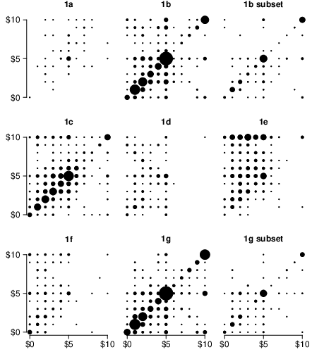
| Figure 1: Results of studies 1a-g. The figure plots bet valuations
(x-axis) against hedge valuations (y-axis) for the seven experiments
and two separately analyzed subsets
summarized in Table 1. Dot area is proportional
to number of participants at each coordinate. Note that 1f
actually ranged from $0 to $100, but is re-scaled to match other
studies in this figure. (see
Appendix B for
materials). |
| Table 2: Materials for Studies 2a and 2b. |
| 2a (N=297) | 2b
(N=299) |
Suppose a fair coin is going to be flipped once.
A “HEADS Voucher” pays out $10 if the coin lands heads.
A “TAILS Voucher” pays out $10 if the coin lands
tails.
Which would you rather have?
A) A HEADS voucher and a TAILS voucher 66%
B) A HEADS voucher and a five dollar bill 34%
Which would you rather have?
A) A HEADS voucher 30%
B) A five dollar bill 70% | | Suppose a fair coin is going to be flipped once.
A “HEADS Voucher” pays out $10 if the coin lands heads.
A “TAILS Voucher” pays out $10 if the coin
lands tails.
Which would you rather have?
A) A HEADS voucher and a TAILS voucher, so that you make $10
if the coin lands heads and $10 if the coin lands tails
74%
B) A HEADS voucher and a five dollar bill, so that you make
$15 if the coin lands heads and $5 if the coin lands tails
26%
Which would you rather have?
A) A HEADS voucher, so that you make $10 if the coin lands
heads and $0 if the coin lands tails 11%
B) A five dollar bill, so that you make $5 if the coin lands
heads and $5 if the coin lands tails
89% |
Studies 2a and 2b
Evaluating Heads and Tails vouchers separately and sequentially partially
obscures their complementarity.5 Thus, in our next two
studies, MTurk workers chose between the pair of vouchers {Heads
& Tails} and the package {Heads & $5} (see Table 2). With this more
transparent
formulation, most did prefer the voucher pair – and thus, at least
implicitly, valued the Tails hedge above its expected value, as risk
aversion dictates.6,7 However, even here, the explanatory
power of risk preference remains in doubt, since those who preferred
{Heads & Tails} to {Heads & $5} should also have preferred a sure
$5 over a single Heads voucher, and vice versa. Yet we observed little
relation between those two choices.8
Study 3
When considered separately, the Heads and Tails vouchers are symmetric:
equivalent and interchangeable. Thus, it is easy to understand why many
respondents value them similarly, even though the first voucher adds
risk and the second removes it. To test whether respondents would
explicitly endorse the symmetry argument over the normative argument,
we presented them side by side (Table 3), with order counterbalanced,
and simply asked respondents to choose one.
| Table 3: Materials for Study 3 |
A fair coin will be flipped once.
A HEADS voucher pays $10 if the coin lands HEADS.
A TAILS voucher pays $10 if the coin lands TAILS.
Bob was willing to pay up to $3 for a HEADS voucher and
purchased one at that price.
How much should he be willing to pay for a TAILS voucher? (So
that he would own both vouchers before the coin is flipped.)
∘ $7 (He should value the pair of vouchers
at $10 because owning both guarantees him $10.)
∘ $3 (He should value each voucher the same because
each offers the same chance of $10.)
|
Only one in ten respondents (53/505) chose the correct argument ($7)
over the symmetry argument ($3). Moreover, this small minority might
actually have been even more confused, as those choosing $7 were
less likely to pass an attention check and did significantly
worse on a numeracy test appended to subsequent demographics
questions (see
Appendix
D).9
Study 4
To slightly generalize our basic paradigm, we next removed the
symmetry between the bet and the hedge. We asked 182 MTurkers how much
they would pay for four different bets: a 20% chance of $100, a 40%
chance of $100, a 60% chance of $100, and an 80% chance of $100
as well as how much they would pay for the four corresponding
hedges (which pay off in the remaining states). All four bet-hedge pairs were
presented to each participant in random order. For each pair, respondents
indicated their valuations of the
bet, and then their valuations of the corresponding hedge. As before,
possession of both guarantees the prize, and thus their two
valuations should sum to $100 and correlate −1.0. However, unlike
before, the bet and hedge are not symmetric, as they have
different probabilities of delivering the prize. The results are
summarized in Figure 2.
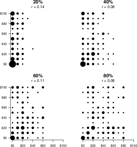
| Figure 2: WTP for a P% chance at $100 and for its perfect
hedge. The figure plots bet valuations (x-axis) against hedge
valuations (y-axis) for each probability of $100 in Study 4. Dot
area is proportional to number of participants at each coordinate. |
With symmetry removed, valuations of the bet and the hedge correlate
much more weakly, though still positively. Again, almost no
data lie along the southeast diagonal, as the two
valuations sum to well below $100 in all four cases. The mean
valuations of the bet and hedge are reported in Table 4, with the
subscript representing the asset’s valuation relative to its expected
value.
A comparison of the subscripts reveals that the bets and hedges
generally deviate in the same direction from expected value
(below it), rather than diverging to reveal a coherent attitude toward
risk. However, though the two valuations do not cohere, hedges are, at
least, valued at a higher fraction of their expected value.
Moreover, respondents are willing to pay more than expected value to
hedge the small residual risk of the 80% bet – providing at least one
instance where a perfect hedge is priced above its expected value
($20), as should be universally expected for respondents who are risk
averse.
| Table 4: Mean bet and hedge valuations. |
21inAsset acquired or hedged | Mean WTP
proportion of EV |
| | Bet | Hedge |
20% of $100 | $6 0.32 | $41 0.51 |
40% of $100 | $15 0.36 | $39 0.66 |
60% of $100 | $22 0.36 | $40 0.99 |
80% of $100 | $34 0.42 | $38
1.91 |
The considerable difference between bet and hedge subscripts in Table
4 suggests that respondents are not simply ignoring
possession of the bet when evaluating the hedge. For instance, they
are willing to pay $6 for a 20% chance of $100 alone, but $38
for the same asset once they already own an 80% chance of $100.
Although respondents clearly
fail to fully appreciate the covariance between bets and hedges, the
pattern remains distinct from complete covariance neglect, in which
hedges and bets are treated as independent.10
Nor are respondents
in earlier “Heads and Tails” studies merely referencing their
valuation of the bet to construct an equivalent valuation of the
hedge. Although a substantial minority of hedge prices do equal bet
prices in
those studies, most don’t. And of the minority that do, many come from
respondents who “simply” report the expected value for each asset ($5, $5).
Though those are certainly reasonable valuations (and demanded by EUT), we
strongly suspect that many of these respondents are treating these questions as
math problems rather than an elicitation of their preferences (and would
continue to just perform the math even if the numbers referenced
millions of dollars). This suspicion draws some support from an
analysis in Appendix C, which
reports the data broken down by CRT score: those who answer ($5, $5)
are no more reflective than off diagonal respondents and less
reflective than the small minority of responses that lie elsewhere on
the southeast diagonal.
In opposition to various “narrow framing” theories (e.g., Tversky &
Kahneman, 1986) that assume respondents ignore possession of the bet when
evaluating the hedge stand “multiple reference point” theories (e.g.,
Koszegi & Rabin, 2006, 2007) in which evaluation of hedge entails
full consideration of both possible outcomes of the bet:
the one in which the bet pays off (in which case money spent on the hedge
is a waste and a loss) and the one in which the bet does not (but
the hedge does, minus acquisition costs). By this multiple reference point
formulation, acquisition of the hedge constitutes both a loss and
a gain, which tends to make an unattractive combination to the extent that
losses loom larger than gains. (See
Appendix E for an
examination of whether the multiple reference point perspective can make
sense of our results. We conclude it cannot.11)
3 Discussion
Valuations of bets and hedges are theoretically equivalent measures of
risk attitudes, yet they often compel opposite conclusions. For
instance, many who place a low value on risk-creating bets also place a
low value on risk-reducing hedges. This marked departure from
theoretical expectations seemingly impugns the construct validity of
risk attitudes – even within the narrow domain of stylized
monetary gambles. Of course, identifying
discrepancies between a subset of measurement techniques isn’t usually
regarded as sufficient cause to jettison a theoretically cherished
construct – at least not within the social sciences. Nevertheless, to
the extent that the two measures depart, it certainly raises the question
about which, if either, better captures whatever we think we mean by
risk aversion.
Adjudicating between potential measures of a putative construct requires
the very thing that is lacking for constructs whose validity is still
in question – agreement about the other thing(s) with which we should
expect them to correlate. For instance, suppose Holt and Laury’s (2002)
measure of risk preferences had corresponded much more highly
with hedge valuations than with bet valuations. The conclusions drawn
from this will still be conditioned by your prior faith in those
measures. If you are confident that Holt and Laury’s measure
captures the construct you care about, it would affirm hedge valuations
and impugn bet valuations, but if you are confident that bet valuations
best capture risk attitudes, the lack of relation with that other method would
impugn that method.
In the experimental paradigm we use most commonly, the hedges are
perfect, such that possession of one renders the coin irrelevant. This
evokes the image of a very unusual transaction in which an owner of the
bet pays $7 for the hedge and is then immediately handed $10. Since
this is obviously equivalent to simply receiving $3, buying the hedge
is equivalent to selling the bet. But the value of a perfect hedge also
determines the aggregate value of the partial hedges from which it
might be constructed. Consider
an experiment in which chances to win a $100 prize can be
purchased in cumulative increments of one percentage point each; a
single point entitles its owner to a 1% chance of $100; fifteen
points yields a 15% chance of $100, and so on. The expected value of
each 1% chance is, of course, $1. Now consider a respondent for whom
a 50% chance of winning a $100 prize is worth $30. That person
values the first 50 points at 60 cents each, on average.
However, since the next 50 points must be worth $70 in total,
their average value must be $1.40. Moreover, if any of the incremental
percentage points beyond 50% are also valued below $1.00, achieving
that $1.40 average requires that valuation of later
increments exceed $1.40. In other words, continuity demands
that these partial hedges must eventually be worth much more than their
expected value – and this point will typically come well before one has
acquired a 100% chance of winning.
Note further that once a prize becomes more likely than not, additional
increases in the chances of winning reduce variance at an
accelerating rate. Since aversion to variance dominates every formal
definition of risk aversion, those who are risk averse should often
treat partial hedges like perfect hedges – as variance reducing assets
that are worth even more than their expected value. Thus, assets that
eliminate risk, like Tails vouchers, are an illustrative case,
but not a special case.
The construct of risk aversion seemingly draws support from the
popularity of insurance contracts, on which U.S. customers alone spend
over a trillion dollars a year.12
However, while people typically insure against their house catching
fire, they rarely insure against a decline in house prices, though
home equity comprises most of a household’s net worth
at retirement.13 Moreover, analogous contracts that extract a premium
to reduce the variability of uncertain gains are also
rare.14
Thus, as Friedman et al. (2014) point out, while insurance contracts
are typically invoked as evidence of risk aversion, customer behavior
actually departs from textbook risk aversion; customers appear
motivated to reduce the possibility of some types of harm, rather than
reduce variance, per se. This distinction between downside
risk and upside risk raises further questions about how subjects in
our experiments interpret an actuarially unfair hedge: as an
attractive premium to limit losses from unfavorable
realizations of their risky asset (e.g., spending $700,000 on
insurance to guard against the 50% chance their million dollar house
will burn down) or as an unattractive censoring of the upside of their
risky asset (e.g., as guaranteeing a mere $300,000 when they know
their house will be worth a million if it does not burn
down).
When we’ve presented this research, the most common objection is that
respondents are just confused. We “concede” that, at some
level, they are. For instance, consider the common response of someone
who indicates they’d pay up to $3 for the bet and up to $3
for a hedge (if they had purchased or were endowed with the bet). This,
in turn implies they’d pay up to $6 for both, but not, say,
$7.50. But since the bet and hedge are worth $10 in combination,
their responses imply they would decline receiving $2.50 if you
attempted to hand it to them. This is obviously false and so their
answer is, in an important sense, a mistake. And this mistake persists
even when participants are explicitly given the normative explanation,
as in Study 3. However, we see these mistakes as the
phenomenon of interest. We don’t doubt
that after a sufficiently intense and prolonged training session
respondents could generate a normative pair of valuations, much as they
could be taught to use Venn Diagrams or apply Bayes' Rule, or produce
normative responses in many other contexts. But this doesn’t vitiate
the phenomenon nor remove the challenges it poses to conceptions of
risk attitudes.
References
Barber, B., & Odean, T. (2000). Trading is hazardous to your wealth:
The common stock investment performance of individual
investors. Journal of Finance, 55, 773–806.
Barseghyan, L. Prince, J., & Teitelbaum, J. C. (2011). Are risk
preferences stable across contexts?
Evidence from insurance data. American Economic Review,
101, 591–631.
Barsky, R. B., Juster, T., Kimball, M., & Shapiro, M. (1997). Preference
parameters and behavioral heterogeneity: An experimental approach in the
health and retirement study. Quarterly Journal of
Economics, 112, 537–579.
Benartzi, S. & Thaler, R. H. (2001). Naïve diversification strategies
in defined contribution saving plans, American Economic Review,
91, 79–98.
Brown, J. R. (2009). Understanding the role of annuities in retirement
planning. In A. Lusardi (Ed.), Overcoming the savings slump: How to
increase the effectiveness of financial education and saving
programs, pp. 178–206. University of Chicago Press.
Charness, G., Gneezy, U., & Imas, A. (2013). Experimental methods: Eliciting
risk preferences. Journal of Economic Behavior & Organization, 87,
43-51.
Choi, J. J., Laibson, D., & Madrian, B. C. (2005). Are empowerment and
education enough? Underdiversification in 401(k) plans.
Brookings Papers on Economic Activity 2005, 2, 151–198.
Choi, J. W., & Lee, J. M. (2015). Housing futures markets. In
The World Scientific Handbook of Futures Markets, 15,
465–485.
Cornil, Y., & Bart, Y. (2013). The diversification paradox: Covariance
information and risk perception among lay investors. Unpublished
manuscript. [Singapore: INSEAD Working Paper Series, 1-45.]
Cutler, D. M., & Glaeser, E., (2005). What explains differences in
smoking, drinking, and other health-related behaviors? American
Economic Review, 95, 238–242.
Einav, L., Finkelstein, A., Pascu, I., & Cullen, M. (2012). How general
are risk preferences? Choices under uncertainty in different domains.
American Economic Review, 102, 2606–2638.
French, K. R., & Poterba, J. M. (1991). Investor diversification and
international equity markets. American Economic Review,
81, 222–226.
Frederick, S. (2005). Cognitive reflection and decision making.
Journal of Economic Perspectives, 19, 25–42.
Friedman, D., Isaac, R. M., James, D., & Sunder, S. (2014). Risky
curves: On the empirical failure of expected utility. Routledge.
Grinblatt, M., & Keloharju, M. (2001). How distance, language, and
culture influence stockholdings and
trades. Journal of Finance, 56, 1053–1073.
Holt, C. A., & Laury, S. K. (2002). Risk aversion and incentive
effects. American Economic Review, 92, 1644–1655.
Huberman, G. (2001). Familiarity breeds investment. Review of
Financial Studies, 14, 659–680.
Kahneman, D., & Tversky, A. (1979). Prospect theory: An analysis of
decision under risk. Econometrica, 47, 263–291.
Kőszegi, B., & Rabin, M. (2006). A model of reference-dependent
preferences. The Quarterly Journal of Economics, 121,
1133–1165.
Kőszegi, B., & Rabin, M. (2007). Reference-dependent risk
attitudes. American Economic Review, 97, 1047–1073.
Markle, A. B., & Rottenstreich, Y. (2018). Simultaneous preferences for
hedging and doubling down: Focal prospects, background positions, and
nonconsequentialist conceptualizations of uncertainty.
Management Science, https://doi.org/10.1287/mnsc.2017.2918.
Meulbroek, L. (2002). Company stock in pension plans: How costly is it?
Unpublished manuscript.
Poterba, J. M. (2014). Retirement security in an aging population.
American Economic Review, 104, 1–30.
Rabin, M. (2000). Risk aversion and expected-utility theory: A
calibration theorem. Econometrica, 68, 1281–1292.
Rabin, M, & Thaler, R. H. (2001). Anomalies: Risk aversion.
Journal of Economic Perspectives, 15, 219–232.
Reinholtz, N., Fernbach, P., & Langhe, B. D. (2018). Do people
understand the benefit of diversification? Available at SSRN 2719144.
Thaler, R. H., & Johnson, E. J. (1990). Gambling with the house money
and trying to break even: The effects of prior outcomes on risky
choice. Management science, 36, 643–660.
Tversky, A., & Kahneman, D. (1986). Rational choice and the framing of
decisions. Journal of Business, S251-S278.
Welch, I. (2001) The top achievements, challenges, and failures of
finance. Unpublished Manuscript. [Yale ICF Working Paper Series, No.
00–67.]
This document was translated from LATEX by
HEVEA.