Judgment and Decision
Making, vol. 1, no. 2, November 2006, pp. 108-117.
Probability biases as Bayesian inference
André C. R. Martins1
Universidade de São Paulo
Abstract
In this article, I will show how several observed biases in
human probabilistic reasoning can be partially explained as
good heuristics for making inferences in an environment where
probabilities have uncertainties associated to them. Previous
results show that the weight functions and the observed
violations of coalescing and stochastic dominance can be
understood from a Bayesian point of view. We will review those
results and see that Bayesian methods should also be used as
part of the explanation behind other known biases. That means
that, although the observed errors are still errors under the
laboratory conditions in which they are demonstrated, they can %XX
be understood as adaptations to the solution of real life
problems. Heuristics that allow fast evaluations and mimic a
Bayesian inference would be an evolutionary advantage, since
they would give us an efficient way of making decisions.
Keywords: weighting functions, probabilistic biases, adaptive probability theory.
1 Introduction
It is a well known fact that humans make mistakes when presented
with probabilistic problems. In the famous paradoxes of Allais
(1953) and Ellsberg (1961), it was observed that, when faced with
the choice between different gambles, people make their choices
in a way that is not compatible with normative decision theory.
Several attempts to describe this behavior exist in the
literature, including Prospect Theory (Kahneman & Tversky,
1979), Cumulative Prospect Theory (Kahneman & Tversky, 1992),
and a number of configural weighting models (Birnbaum & Chavez,
1997; Luce, 2000; Marley & Luce, 2001). All these models use
the idea that, when analyzing probabilistic gambles, people alter
the stated probabilistic values using a S-shaped weighting
function w(p) and use these altered values in order to
calculate which gamble would provide a maximum expected return.
Exact details of all operations involved in these calculations,
as values associated to each branch of a bet, coalescing of equal
branches, or aspects of framing are dealt with differently in
each model, but the models agree that people do not use the exact
known probabilistic values when making their decisions. There are
also models based on different approaches, as the decision by
sampling model. Decision by sampling proposes that people make
their decision by making comparisons of attribute values
remembered by them and it can describe many of the
characteristics of human reasoning well (Stewart et al., 2006).
Recently, strong evidence has appeared indicating that the
configural weighting models describe human behavior better than
Prospect Theory. Several tests have shown that people don't obey
simple decision rules. If a bet is presented with two equal
possible outcomes, for example, 5% of chance of getting 10 in
one outcome and 10% of chance of getting the same return, 10, in
another possible result, it should make no difference if both
outcomes were combined into one single possibility, that is, a 15%
chance of obtaining 10. This property is called coalescing of
branches and it has been observed that it is not always respected
(Starmer & Sugden, 1993; Humphrey, 1995; Birnbaum, 2004).
Other strong requirement of decision theory that is violated in
laboratory experiments is that people should obey stochastic
dominance. Stochastic dominance happens when there are two bets
available and the possible gains of one of them are as good as
the other one, with at least one possibility to gain more. Per
example, given the bets G=$96,0.9; $12,0.1 and
G+=$96,0.9; $14,0.05; $12,0.05, G+ clearly dominates
G, since the first outcome is the same and the second outcome
in G is split into two possibilities in G+, returning the
same or more than G, depending on luck. The only rational
choice here is G+, but laboratory tests show that people do not
always follow this simple rule (Birnbaum, 1999). Since
rank-dependent models, as Prospect Theory (and Cumulative
Prospect Theory) obey both stochastic dominance and coalescing of
branches, configural weight models, that can predict those
violations, are probably a better description of real behavior.
In the configural weight models, each branch of a bet is given a
different weight, so that the branches with worst outcome will be
given more weight by the decider. This allows those basic
principles to be violated. However, although configural weight
models can be good descriptive models, telling how we reason, the
problem of understanding why we reason the way we do is not
solved by them. The violations of normative theory it predicts
are violations of very simple and strong principles and it makes
sense to ask why people would make such obvious mistakes.
Until recently, the reason why humans make these mistakes was
still not completely clear. Evolutionary psychologists have
suggested that it makes no sense that humans would have a module
in their brains that made wrong probability assessments (Pinker,
1997), therefore, there must be some logical explanation for
those biases. It was also suggested that, since our ancestors had
to deal with observed frequencies instead of probability values,
the observed biases might disappear if people were presented with
data in the form of observed frequencies in a typical Bayes
Theorem problem. Gigerenzer and Hoffrage (1995) conducted an
experiment confirming this idea. However, other studies checking
those claims (Griffin, 1999; Sloman, 2003) have shown that
frequency formats seem to improve the reasoning only under some
circumstances. If those circumstances are not met, frequency
formats have either no effect or might even cause worse
probability evaluations by the tested subjects.
On the other hand, proponents of the heuristics and biases point
of view claim that, given that our intellectual powers are
necessarily limited, errors should be expected and the best one
can hope is that humans would use heuristics that are efficient,
but prone to error (Gigerenzer & Goldstein, 1996). And, as a
matter of fact, they have shown that, for decision problems,
there are simple heuristics that do a surprisingly good job
(Martignon, 2001). But, since many of the calculations involved
in the laboratory experiments are not too difficult to perform,
the question of the reasons behind our probabilistic reasoning
mistakes still needed answering. If we are using a reasonable
heuristics to perform probabilistic calculations, understanding
when this is a good heuristic and why it fails in the tests is an
important question.
Of course, the naïve idea that people should simply use
observed frequencies, instead of probability values, can
certainly be improved from a Bayesian point of view. The argument
that our ancestors should be well adapted to deal with
uncertainty from their own observations is quite compelling, but,
to make it complete, we can ask what would happen if our
ancestors minds (and therefore, our own) were actually more sophisticated than a simple frequentistic mind. If they had
a brain that, although possibly using rules of thumb, behaved in
a way that mimicked a Bayesian inference instead of a
frequentistic evaluation, they would be better equipped to make
sound decisions and, therefore, that would have been a good
adaptation. In other words, our ancestors who were
(approximately) Bayesians would be better adapted than any
possible cousins who didn't consider uncertainty in their
analysis. And that would eventually lead those cousins to
extinction. Of course, another possibility is that we learn those
heuristics as we grow up, adjusting them to provide better
answers. But, even if this is the dynamics behind our heuristics,
good learning should lead us closer to a Bayesian answer than afrequentistic one. So, it makes sense to ask if humans are
actually smarter than the current literature describes them as.
Evidence supporting the idea that our reasoning resembles
Bayesian reasoning already exists. Tenenbaum et al. (in press)
have shown that observed inductive reasoning can be modeled by
theory-based Bayesian models and that those models can provide
approximately optimal inference. Tests of human cognitive
judgments about everyday phenomena seems to suggest that our
inferences provide a very good prediction for the real statistics
(Griffiths & Tenenbaum, 2006).
1.1 Adaptive probability theory (APT)
In a recent work (Martins, 2005), I have proposed the Adaptive
Probability Theory (APT). APT claims that the biases in human
probabilistic reasoning can be actually understood as an
approximation to a Bayesian inference. If one supposes that people treat all probability values as if they were uncertain (even when they are not) and make some assumptions
about the sample size where those probabilities would have been
observed as frequencies, it follows that the observed shape of
the weighting functions is obtained. Here, I will review those
results and also show that we can extend the ideas that were
introduced to explain weighting functions to explain other
observed biases. I will show that some of those biases can be
partially explained as a result of a mind adapted to make inferences in an environment where probabilities have
uncertainties associated to them. That is, the weighting
functions of Prospect Theory (and the whole class of models that
use weighting functions to describe our behavior) can be
understood and predicted from a Bayesian point of view. Even the
observed violations of descriptive Prospect Theory, that is,
violations of coalescing and stochastic dominance, that need
configural weight models to be properly described, can also be
predicted by using APT. And I will propose that Bayesian methods
should be used as part of the explanation behind a number of
other biases (for a good introductory review to many of the
reported mistakes, see, for example, Plous, 1993).
1.2 What kind of theory is APT?
Finally, a note on what APT really is, from an epistemological
point of view, is needed. Usually, science involves working on
theories that should describe a set of data, making predictions
from those theories and testing them in experiments. Decision
theory, however, requires a broader definition of proper
scientific work. This happens because, unlike other areas, we
have a normative decision theory that tells us how we should
reason. It does not necessarily describe real behavior, since it
is based on assumptions about what the best choice is, not about
how real people behave. Its testing is against other decision
strategies and, as long as it provides optimal decisions, the
normative theory is correct, even if it does not predict behavior
for any kind of agents. That means that certain actions can be
labeled as wrong, in the sense that they are far from optimal
decisions, even though they correspond to real actions of real
people.
This peculiarity of decision theory means that not every model
needs to actually predict behavior. Given non-optimal observed
behavior, understanding what makes the deciders to behave that
way is also a valid line of inquiry. That is where APT stands.
Its main purpose is to show that apparently irrational behavior
can be based on an analysis of the decision problem that follows
from normative theory. The assumptions behind such analysis might
be wrong and, therefore, the observed behavior would not be
optimal. That means that our common sense is not perfect.
However, if it works well for most real life problems, it is
either a good adaptation or well learned. APT intends to make a
bridge between normative and descriptive theories. This means
that it is an exploratory work, in the sense of trying to
understand the problems that led our minds to reason the way they
do. While based on normative theory, it was designed to agree
with the observed biases. This means that APT does not claim to
be the best actual description of real behavior (although it
might be). Even if other theories (such as configural weight
models or decision by sampling) actually describe correctly the
way our minds really work, as long as their predictions are compatible with APT, APT will show that the actual behavior
predicted by those theories is reasonable and an approximation to
optimal decisions. Laboratory tests can show if APT is actually
the best description or not and we will see that APT suggests new
experiments in the problem of base rate neglect, in order to
understand better our reasoning. But the main goal of APT is to
show that real behavior is reasonable and it does that well.
2 Bayesian weighting functions
Suppose you are an intuitive Bayesian ancestor of mankind (or a
Bayesian child learning how to reason about the world). That is,
you are not very aware of how you decide the things you do, but
your mind does something close to Bayesian estimation (although
it might not be perfect). You are given a choice between the
following two gambles:
| Gamble A | Gamble B |
| 85% to win 100 | 95% to win 100 |
| 15% to win 50 | 5% to win 7
|
If you are sure about the stated probability values and you are
completely rational, you should just go ahead and assign
utilities to each monetary value and choose the gamble that
provides the largest expected utility. And, as a matter of fact,
the laboratory experiments that revealed the failures in human
reasoning provided exact values, without any uncertainty
associated to them. Therefore, if humans were perfect Bayesian
statisticians, when faced with those experiments, the subjects
should have treated those values as if they were known for sure.
But, from your point of view of an intuitive Bayesian, or from
the point of view of everyday life, there is no such a thing as a
probability observation that does not carry with it some degree
of uncertainty. Even values from probabilistic models based on
some symmetry of the problem depend, in a more complete analysis,
on the assumption that the symmetry does hold. If it doesn't, the
value could be different and, therefore, even though the
uncertainty might be small, we would still not be completely sure
about the probability value.
Assuming there is uncertainty, what you need to do is to obtain
your posterior estimate of the chances, given the stated gamble
probabilities. Here, the probabilities you were told are actually
the data you have about the problem. And, as long as you were not
in a laboratory, it is very likely they have been obtained as
observed frequencies, as proposed by the evolutionary
psychologists. That is, what you understand is that you are being
told that, in the observed sample, a specific result was observed
85% of the times it was checked. And, with that information in
mind, you must decide what posterior value it will use.
The best answer would certainly involve a hierarchical model
about possible ways that frequency was observed and a lot of
integrations over all the nuisance parameters (parameters you are
not interested about). You should also consider whether all
observations were made under the same circumstances, if there is
any kind of correlation between their results, and so on. But all
those calculations involve a cost for your mind and it might be a good idea to accept simpler estimations that work reasonably
well most of the time. You are looking for a good heuristic, one that
is simple and efficient and that gives you correct answers most
of the time (or, at least, close enough). That is the basic idea
behind Adaptive Probability Theory (Martins, 2005). Our minds, from evolution or learning, are built to work with probability
values as if they were uncertain and make decisions compatible
with that possibility. APT does not claim we are aware of that,
it just says that our common sense is built in a way that mimics
a Bayesian inference of a complex, uncertain problem.
If you hear a probability value, it is a reasonable assumption to
think that the value was obtained from a frequency observation.
In that case, the natural place to look for a simple heuristic is
by treating this problem as one of independent, identical
observations. In this case, the problem has a binomial likelihood
and the solution to the problem would be straight-forward if not
for one missing piece of information. You were informed the
frequency, but not the sample size n. Therefore, you must use
some prior opinion about n.
In the full Bayesian problem, that means that n is a nuisance
parameter. This means that, while inference about p is desired,
the posterior distribution depends also on n and the final
result must be integrated over n. The likelihood that a
observed frequency o, equivalent to the observation of s=no
successes, is reported is given by
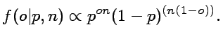 (1)
(1)
In order to integrate over n, a prior for it is required.
However, the problem is actually more complex than that since it
is reasonable that our opinion on n should depend on the value
of o. That happens because if o=0.5, it is far more likely
that n=2 than if o=0.001, when it makes sense to assume that
at least 1,000 observations were made. And we should also
consider that extreme probabilities are more subject to error.
In real life, outside the realm of science, people rarely, if
ever, have access to large samples to draw their conclusions
from. For the problem of detecting correlates, there is some
evidence that using small samples can be a good heuristics
(Kareev, 1997). In other words, when dealing with extreme
probabilities, we should also include the possibility that the
sample size was actually smaller and the reported frequency is
wrong.
The correct prior f(n,o), therefore, can be very difficult to
describe and, for the complete answer, hierarchical models
including probabilities of error are needed. However, such a
complicated, complete model is not what we are looking for. A
good heuristic should be reasonably fast to use and shouldn't depend on too many details of the model. Therefore,
it makes sense to look for reasonable average values of n and
simply assume that value for the inference process.
Given a fixed value for n, it is easy to obtain a posterior
distribution. The likelihood in Equation 1 is
a binomial likelihood and the easiest way to obtain inferences
when dealing with binomial likelihoods is assuming a Beta
distribution for the prior. Given a Beta prior with parameters
a and b, the posterior distribution will also be a Beta
distribution with parameters a+s and b+n. The average of a
random variable that follows a Beta distribution with parameters
a and b has a simple form, [a/(a+b)]. That means that
we can obtain a simple posterior average for the probability p,
given the observed frequency o, w(o)=E[p|o]
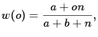 (2)
(2)
which is a straight line if n is a constant (independent of
o), but different and less inclined than w(o)=o. For a
non-informative prior distribution, that corresponds to the
choice a=1 and b=1, Equation 2 can be written in
the traditional form (1+s)/(2+n) (Laplace rule).
However, a fixed sample size, equal for all values of p does
not make much sense in the regions closer to certainty and n
must somehow increase as we get close to those regions
(o® 0 or o® 1). The easiest way to model
n is to suppose that the event was observed at least once (and,
at least once, it was not observed). That is, if o is small,
choose an observed number of successes s=1 (some other value
would serve, but we should remember that humans tend to think
with small samples, as observed by Kareev et al., 1997). If p
is closer to 1, take s=n-1. That is, the sample size will be
given by n=1/t where t=min(o;1-o) and we have that
w(o)=2o/(2o+1) for o < 0.5 and w(o)=1/(3-2o) for o > 0.5. By
calculating
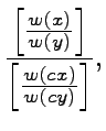
it is easy to show that the common-rate effect holds, meaning
that the curves are subproportional, both for o < 0.5 and
o > 0.5. Estimating the above fraction shows that
w(x)/w(y) < w(cx)/w(cy), for c < 1, exactly when x < y. The curve
w(o) can be observed in Figure , where it is
compared to a curve proposed by Prelec (2000) as a
parameterization that fits reasonably well the data observed in
the experiments.
A few comments are needed here. For most values of o, the
predicted value of n will not be an integer, as it would be
reasonable to expect. If o=0.4, we have n=2.5, an odd and
absurd sample size, if taken literally. One could propose using a
sample size of n=5 for this case, but that would mean a
non-continuous weighting function. More than that, for too
precise values, as 0.499, that would force n to be as large
as 1.000. However, it must be noted that, in the original
Bayesian model, n is not supposed to be an exact value, but the
average value that is obtained after it is integrated out
(remember it is a nuisance parameter). As an average value, there
is nothing wrong with non-integer numbers. Also, it is necessary
to remember that this is a proposed heuristic. It is not the
exact Bayesian solution to the problem, but an approximation to
it. In the case of o=0.499, it is reasonable to assume that
people would interpret it as basically 50%. In that sense, what
the proposed behavior for n says is that, around 50%, the
sample size is estimated to be around n=2; around o=0.33, n
is approximately 3; and so on.
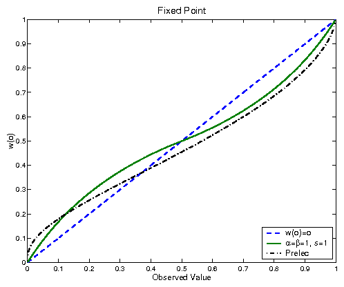 Figure 1: Weighting Function as a function of observed frequency. The curve proposed by Prelec, fitted to the observed data, as well as the w(o)=o curve are also shown for comparison.
The first thing to notice in Figure 1 is that, by
correcting the assumed sample size as a function of o, the
S-shaped format of the observed behavior is obtained. However,
there are still a few important quantitative differences between
the observations and the predicted curve. The most important one
is on the location of the fixed point of, defined as the
solution to the equation w(o)=o. If we had no prior information
about o (a=b=1), we should have of=0.5. Instead, the
actual observed value is closer to 1/3. That is, for some
reason, our mind seems to use an informative prior where the probability associated with obtaining the better outcomes are
considered less likely than those associated with the worse
outcomes (notice that the probability o is traditionally
associated with the larger gain in the experiment). As a matter
of fact, configural weighting models propose that, given a
gamble, the branches with worst outcomes are given more weight
than those with higher returns. For gambles with two branches,
the lower branch is usually assigned a weight around 2, while the
upper branch has a weight of 1. This can be understood as risk
management or also as some lack of trust. If someone offered you
a bet, it is possible that the real details are not what you are
told and it would make sense to consider the possibility that the
bet is actually worse than the described one.
Figure 1: Weighting Function as a function of observed frequency. The curve proposed by Prelec, fitted to the observed data, as well as the w(o)=o curve are also shown for comparison.
The first thing to notice in Figure 1 is that, by
correcting the assumed sample size as a function of o, the
S-shaped format of the observed behavior is obtained. However,
there are still a few important quantitative differences between
the observations and the predicted curve. The most important one
is on the location of the fixed point of, defined as the
solution to the equation w(o)=o. If we had no prior information
about o (a=b=1), we should have of=0.5. Instead, the
actual observed value is closer to 1/3. That is, for some
reason, our mind seems to use an informative prior where the probability associated with obtaining the better outcomes are
considered less likely than those associated with the worse
outcomes (notice that the probability o is traditionally
associated with the larger gain in the experiment). As a matter
of fact, configural weighting models propose that, given a
gamble, the branches with worst outcomes are given more weight
than those with higher returns. For gambles with two branches,
the lower branch is usually assigned a weight around 2, while the
upper branch has a weight of 1. This can be understood as risk
management or also as some lack of trust. If someone offered you
a bet, it is possible that the real details are not what you are
told and it would make sense to consider the possibility that the
bet is actually worse than the described one.
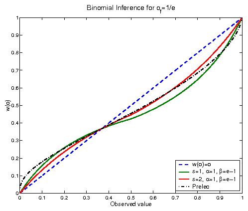 Figure 2: Weighting Functions as a function of observed frequency for a binomial likelihood with fixed point of=1/e
A different fixed point can be obtained by assigning different
priors, that is if a, in the Beta distribution, correspond to
the upper branch and b to the lower one, keep using a=1 and
change the value of b for something larger. Following the
suggestion that of=1/e (Prelec, 2000), based on compound
invariance, we have a=1 and b=e-1. This values are not
necessarily exact and they can also be understood as giving more
weight to the worse outcome. That choice would be reasonable if
there was any reason to believe that the chances might actually
be worse than the stated probability values.
Figure 2 shows the results for this informative
prior, with the s=1 (n-1 for p > 0.5) and s=2 (or n-2)
curves.
This change leads to a posterior average w(o) with a correct
fixed point, but the predicted curve does not deviate from the
w(o)=o curve as much as it has been observed. This is
especially true for values of o near the certainty values,
where the effect should be stronger, due to what is known as
certainty effect (Tversky & Kahneman, 1981). The certainty
effect is the idea that when a probability changes from certainty
to almost certain, humans change their decisions about the
problem much more than decision theory tells they should. This
means that the real curve should approach 0 and 1 with larger
derivatives than the ones obtained from the simple binomial
model. In order to get a closer agreement, other effects must be
considered. Martins (2005) has suggested a number of possible
corrections to the binomial curve. Among them, there is a
possibility that the sample size does not grow as fast as it
should when one gets closer to certainty (changing as tg,
instead of t1). Another investigated explanation is that
people might actually be using stronger priors. The curves
generated from those hypotheses are similar to those of
Figure 2. The main effect of the different
parametrizations is on how the weighting function behaves as one
gets closer to certainty. Simple stronger priors (a=3,
b=3(e-1)) do not actually solve the certainty effect, while
slowly growing sample sizes seem to provide a better fitting.
This agrees with the idea that people tend to use small samples
for their decisions. Large samples are costly to obtain and it
makes sense that most everyday inferences are based on small
samples, even when the stated probability would imply a larger
one. And it is important to keep in mind that what is being
analyzed here are possible heuristics and in what sense they
actually agree with decision theory. That mistakes are still made
is nothing to be surprised about.
This means that APT is able to explain the reasons behind the
shape of the weighting functions. As such, APT is also capable of
explaining the observed violations of coalescing and stochastic
dominance. For example, suppose that you have to choose between
the two gambles A and B. One of the possibilities in gamble A is
a branch that gives you a 85% chance to win 100. If gamble A
is changed to a gamble A', where the only change is that this
branch is substituted for two new branches, the first with 5%
to win 100 and the second with 80% to win 100, no change was
actually made to the gamble, if those values are known for sure.
Both new branches give the same return and they can be added up
back to the original gamble. In other words, the only difference
between the gambles is the coalescing of branches. Therefore, if
only coalescing (or splitting) of branches is performed to
transform A into A', people who chose A over B, should still
choose A' over B. However, notice that, the game A has its most
extreme probability value equal to 15%, while in A', it is 5%.
If people behave in a way that is consistent with APT, that means
they will use different sample sizes. And they will make
different inferences. It should not be a surprise, therefore,
that, under some circumstances, coalescing would be broken. Of
course, coalescing is not broken for every choice, but APT, by
using the supposition that the sample grows slower than it should
(g around 0.3) does predict violation of coalescing in the
example reported by Birnbaum (2005). The assumption about sample
sizes will also affect choices where one gamble clearly dominates
the other and, therefore, Martins (2005) has shown that APT can
explain the observed violations of coalescing and stochastic
dominance.
Figure 2: Weighting Functions as a function of observed frequency for a binomial likelihood with fixed point of=1/e
A different fixed point can be obtained by assigning different
priors, that is if a, in the Beta distribution, correspond to
the upper branch and b to the lower one, keep using a=1 and
change the value of b for something larger. Following the
suggestion that of=1/e (Prelec, 2000), based on compound
invariance, we have a=1 and b=e-1. This values are not
necessarily exact and they can also be understood as giving more
weight to the worse outcome. That choice would be reasonable if
there was any reason to believe that the chances might actually
be worse than the stated probability values.
Figure 2 shows the results for this informative
prior, with the s=1 (n-1 for p > 0.5) and s=2 (or n-2)
curves.
This change leads to a posterior average w(o) with a correct
fixed point, but the predicted curve does not deviate from the
w(o)=o curve as much as it has been observed. This is
especially true for values of o near the certainty values,
where the effect should be stronger, due to what is known as
certainty effect (Tversky & Kahneman, 1981). The certainty
effect is the idea that when a probability changes from certainty
to almost certain, humans change their decisions about the
problem much more than decision theory tells they should. This
means that the real curve should approach 0 and 1 with larger
derivatives than the ones obtained from the simple binomial
model. In order to get a closer agreement, other effects must be
considered. Martins (2005) has suggested a number of possible
corrections to the binomial curve. Among them, there is a
possibility that the sample size does not grow as fast as it
should when one gets closer to certainty (changing as tg,
instead of t1). Another investigated explanation is that
people might actually be using stronger priors. The curves
generated from those hypotheses are similar to those of
Figure 2. The main effect of the different
parametrizations is on how the weighting function behaves as one
gets closer to certainty. Simple stronger priors (a=3,
b=3(e-1)) do not actually solve the certainty effect, while
slowly growing sample sizes seem to provide a better fitting.
This agrees with the idea that people tend to use small samples
for their decisions. Large samples are costly to obtain and it
makes sense that most everyday inferences are based on small
samples, even when the stated probability would imply a larger
one. And it is important to keep in mind that what is being
analyzed here are possible heuristics and in what sense they
actually agree with decision theory. That mistakes are still made
is nothing to be surprised about.
This means that APT is able to explain the reasons behind the
shape of the weighting functions. As such, APT is also capable of
explaining the observed violations of coalescing and stochastic
dominance. For example, suppose that you have to choose between
the two gambles A and B. One of the possibilities in gamble A is
a branch that gives you a 85% chance to win 100. If gamble A
is changed to a gamble A', where the only change is that this
branch is substituted for two new branches, the first with 5%
to win 100 and the second with 80% to win 100, no change was
actually made to the gamble, if those values are known for sure.
Both new branches give the same return and they can be added up
back to the original gamble. In other words, the only difference
between the gambles is the coalescing of branches. Therefore, if
only coalescing (or splitting) of branches is performed to
transform A into A', people who chose A over B, should still
choose A' over B. However, notice that, the game A has its most
extreme probability value equal to 15%, while in A', it is 5%.
If people behave in a way that is consistent with APT, that means
they will use different sample sizes. And they will make
different inferences. It should not be a surprise, therefore,
that, under some circumstances, coalescing would be broken. Of
course, coalescing is not broken for every choice, but APT, by
using the supposition that the sample grows slower than it should
(g around 0.3) does predict violation of coalescing in the
example reported by Birnbaum (2005). The assumption about sample
sizes will also affect choices where one gamble clearly dominates
the other and, therefore, Martins (2005) has shown that APT can
explain the observed violations of coalescing and stochastic
dominance.
3 Other biases
It is an interesting observation that our reported mistakes can
be understood as an approximation to a Bayesian inference
process. But if that is true, the same effect should be able to
help explain our observed biases in other situations, not only
our apparent use of weighting functions. And, as a matter of
fact, the literature of biases in human judgment has many other
examples of observed mistakes. If we are approximately Bayesians,
it would make sense to assume that the ideas behind APT should be
useful under other circumstances. In this section, I will discuss
a collection of other mistakes that can be, at least partially,
explained by APT. In the examples bellow, a literature trying to
explain those phenomena already exists, so, it is very likely
that the explanations from APT are not the only source of the
observed biases, and I am not claiming that they are. But APT
should, at least, show that our mistakes are less wrong than
previously thought. Therefore, it makes sense to expect a better
fit between normative and descriptive results when uncertainty is
included in the analysis as well as the possibility that some
sort of error or mistake exists in the data. We will see that the
corrections to decision theoretic results derived from those
considerations are consistently in the direction of observed
human departure from rationality.
3.1 Conjunctive events
Cohen et al. (1979) reported that people tend to overestimate
the probability of conjunctive events. If people are asked to
estimate the probability of a result in a two-stage lottery with
equal probabilities in each state, their answer was far higher
than the correct 25%, showing an average value of 45%. Again,
as in the choice between gambles, this is certainly wrong from a
probabilistic point of view. But the correct 25% value is only
true if independence can be assumed and the value 0.5 is actually
known for sure. Real, everyday problems can be more complex than
that. If you were actually unsure of the real probability and
only thought that, in average, the probability of a given outcome
in the lottery was 50%, the independence becomes conditional on
the value of p. The chance that two equal outcomes will obtain
is given by p2. But, if p is unknown, you'd have to
calculate an average estimate for that chance. Supposing a
uniform prior, that is f(p)=1 for 0 £ p £ 1, the expected
value will be
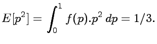
That is, for real problems where only conditional independence
exists, the result is not the correct 25% for the situation
where p is known to be 0.5 with certainty. Of course, if the
uncertainty in the priori was smaller, the result would become
closer to 25%.
Furthermore, if the conditional independence assumption is also
dropped, the predicted results can become even closer to the
observed behavior. In many situations, especially
when little is known about a system,
even conditional independence might be too strong an
assumption. Suppose, for example, that our ancestors needed to
evaluate the probability of finding predators at the river they
used to get water from. If a rational man had a prior uniform
(a=b=1, with an average a/(a+b)=1/2) distribution for the
chance the predator would be there and, after that, only one
observation was made an hour ago where the predator was actually
seen, the average chance a predator would be by the river would
change to a posterior where a=2 and b=1. That is, the average
probability would now be 2/3. However, if he wanted to return to
the river only one hour later, the events would not be
really conditionally independent, as the same predator might
still be there. The existence of correlation between the
observations implies that the earlier sighting of the predator
should increase the probability of observing it there
again. Real problems are not as simple as complete
independence would suggest. Therefore, a good heuristic is not
one that simply multiplies probabilities. When probabilistic
values are not known for sure, true independence does not exist,
only conditional independence remains, and the heuristic should
model that. If our heuristics are also built to include the
possibility of dependent events, they might be more
successful for real problems. However, they would fail more
seriously in the usual laboratory experiments. This means that
the observed estimate for the conjunctive example in Cohen,
around 45%, can be at least partially explained as someone
trying to make inferences when independence, or
even conditional independence, do not necessarily hold.
It is important to keep in mind that our ancestors had to deal
with a world they didn't know how to describe and model as well
as we do nowadays. It would make sense for a successful heuristic
to include the learning about the systems it was applied to. The
notion of independent sampling for similar events might not be
natural in many cases, and our minds might be better equipped by not assuming independence. When faced with the same situation,
not only the previous result can be used as inference for the
next ones, but also it might have happened that some covariance
between the results existed and this might be the origin of the
conjunctive events bias. Of course, this doesn't mean that people
are aware of that nor that our minds perform all the analysis proposed here. The actual calculations can be performed following
different guidelines. All that is actually required is that, most
of the time, they should provide answers that are close to the
correct ones.
3.2 Conservatism
It might seem, at first, that humans are good intuitive Bayesian
statisticians. However, it has been shown that, when faced with
typical Bayesian problems, people make mistakes. This result
seems to contradict APT. One example of such a behavior is
conservatism. Conservatism happens because people seem to update
their probability estimates slower than the rules of probability
dictate, when presented with new information (Phillips &
Edwards, 1966). That is, given the prior estimates and new data,
the data are given less importance than they should have. And,
therefore, the subjective probabilities, after learning the new
information, change less than they should, when compared to a
correct Bayesian analysis. This raises the question of why we
would have heuristics that mimic a Bayesian inference, but
apparently fail to change our points of view by following the
Bayes Theorem.
Described like that, conservatism might sound as a challenge to
APT. In order to explain what might be going on, we need to
understand that APT is not a simple application of Bayesian
rules. It is actually based on a number of different assumptions.
First of all, even though our minds approximate a Bayesian analysis, they do not perform one flawlessly. Second, we have
seen that, when given probabilities, people seem to use sample
sizes that are actually smaller than they should be. And, for any
set of real data, there is always the possibility that some
mistake was made. This possibility exists in scientific works,
subject to much more testing and checking than everyday problems.
For those real problems, the chance of error is certainly larger.
This means that our heuristics should approximate not just a
simple Bayesian inference, but a more complete model. And this
model should include the possibility that the new information
could be erroneous or deceptive. If the probability of deception
or errors, is sufficiently large, the information in the new data
should not be completely trusted. This means that the posterior
estimates will actually change slower than the simpler
calculation would predict. This does not mean that people
actually distrust the reported results, at least, not in a
conscious way. Instead, it is a heuristic that might have evolved in a world where the information available was subject to
all kind of errors.
3.3 Illusory and invisible correlations
Another observed bias is the existence of illusory and invisible
correlations. Chapman and Chapman (1967) observed that people
tended to detect correlations in sets of data where no
correlation was present. They presented pairs of words on a large
screen to the tested subjects, where the pairs were presented
such that each first word was shown an equal number of times
together with each of the different word from the second set.
However, after watching the whole sequence, people tended to
believe that pairs like lion and tiger, or eggs and bacon, showed
up more often than the pairs where there was no logical relation
between the variables. Several posterior studies have confirmed
that people tend to observe illusory correlations when none is
available, if they expect some relation between the variables or
observations for whatever reason.
On the other hand, Hamilton and Rose (1980) observed that, when
no correlation between the variables were expected, it is common
that people will fail to see a real correlation between those two
variables. Sometimes, even strong correlations go unnoticed. And
the experiment also shows that, even when the correlation is
detected, it is considered weaker than the actual one. That is,
it is clear that, whatever our minds do, they do not simply calculate correlations based on the data.
From a Bayesian point of view, this qualitative description of the experiments can not be called an error at all. Translated
correctly, the illusory correlation case simply states that, when
your prior tells you there is a correlation, it is possible that
a set of data with no correlation at all will not be enough to
convince you otherwise. Likewise, if you don't believe a priori
that there is a correlation, your posterior estimate will be
smaller than the observed correlation calculated from the sample.
That is, your posterior distribution will be something between
your prior and the data. When one puts it this way, the result is
so obvious that what is surprising is that those effects have
been labeled as mistakes without any further checks.
Of course, this does not mean that the observed behavior is
exactly a Bayesian analysis of the problem. From what we have
seen so far, it is most likely that it is only an approximation.
In order to verify how people actually deviate from the Bayesian
predictions, we would need to measure their prior opinions about
the problem. But this may not be possible, depending on the
experiment. If the problem is presented together with the data,
people had to make their guesses about priors and update them at
the same time they were already looking at the data (by whatever
mechanism they actually use).
It is important to notice that, once more, the observed biases
were completely compatible with an approximation to a Bayesian
inference. Much of the observed problem in the correlation case
was actually due to the expectation by the experimenters that
people should simply perform a frequentistic analysis and not
include any other information. However, if connections were
apparent between variables, it would be natural to have used an
informative prior, since the honest opinion would be, initially,
that you know something about the correlation. Of course, in
problems where just words are put together, there should be no
reason to expect a correlation. But, for a good heuristic,
detecting a pattern and assuming a correlation can be efficient.
3.4 Base rate neglect
In Section 3.2, we have seen an example of how
humans are not actually accomplished Bayesian statisticians,
since they fail to apply Bayes Theorem in a case where a simple
calculation would provide the correct answer. Another observed
bias where the same effect is observed is the problem of base
rate neglect (Kahneman and Tversky, 1973).
Base rate neglect is the observed fact that, when presented with
information about the relative frequency some events are expected
to happen, people often ignore that information when making
guesses about what they expect to be observed, if other data
about the problem is present. In the experiment where they
observed base rate neglect, Kahneman and Tversky told their
subjects that a group was composed of 30 engineers and 70
lawyers. When presenting extra information about one person of
that group, the subjects, in average, used only that extra
information when evaluating the chance that the person might be
an engineer. Even if the information was non-informative about
the profession of the person, the subjects provided a 50%-50%
of being either an engineer or a lawyer, despite the fact that
lawyers were actually more probable.
Application of APT to this problem is not straight-forward. Since
APT claims that we use approximations to deal with probability problem, one possible approximation is actually
ignore part of the information and use only what the subject
considers more relevant. In the case of those tests, it would
appear that the subjects consider the description of the person
much more relevant than the base rates. Therefore, one possible
approximation is actually ignoring the base rates. If our
ancestors (or the subjects of the experiments, as they grew up)
didn't have access to base rates of most problems they had to
deal with, there would be no reason to include base rates in
whatever heuristics we are using.
On the other hand, it is possible that we actually use the base rates. Notice that base rates are given as frequencies
and, assuming people are not simply ignoring them, those
frequencies would be altered by the weighting functions. In this
problem, a question that must be answered is if there is a worst
outcome. Remember that we can use a non-informative prior
(a=b=1), but, for choice between bets, the fixed point agrees
with a prior information that considers the worse outcome as
initially more likely to happen (a=1 and b=e-1, for example).
In a problem as estimating if someone is an engineer or a lawyer,
the choice of best or worst outcome is non-existent, or
individual, at best. This suggests we should use the
non-informative prior for a first analysis. In order to get a
complete picture, we present the results of calculating weighting
functions for the base rates in Kahneman and Tversky (1973)
experiment in Table . The weighting functions
associated with the observed values of o=30% and o=70% are
presented and two possibilities are considered in the table, that
the sample size grows with 1/t (corresponding to g = 1)
and that it grows slower than it should, with 1/t0.3
(g = 0.3). While the first one would correspond to a more
correct inference, the second alternative (g = 0.3) actually
fits better the observed behavior (Martins, 2005).
Table 1: The result of the weighting functions w(o)
applied to the base rates of Kahneman and Tversky
(1973) experiment, for observed frequencies of
engineers (or lawyers) given by o=0.3 or o=0.7. The
parameter g describes how the sample size n
grows as the observed value o moves towards
certainty.
| | a=b=1 | a=1 and b=e-1 |
|
o=0.3, g = 1 | 0.375 | 0.330 |
| o=0.3, g = 0.3 | 0.416 | 0.344 |
| o=0.7, g = 1 | 0.625 | 0.551 |
| o=0.7, g = 0.3 | 0.584 | 0.483 |
|
|
The first thing to notice in Table 1 is that,
both for observed frequencies of o=0.3 and o=0.7, all
weighting functions provide an answer closer to 0.5 than the
provided base rate. Actually ignoring the base rates correspond
to a prior choice to 0.5, therefore this means that people would
actually behave in a way that is closer to ignoring the base
rates. Notice that, using the case that better describes human
observed choices (g = 0.3) and the fact that there are no
better outcomes here, a=b=1, we get the altered base rates of
0.42 and 0.58, approximately, instead of 0.3 and 0.7. The
correction, once more, leads in the direction of the observed
biases, confirming that APT can play a role in base rate neglect,
even if the base rates are not completelly ignored.
These results also provide an interesting test of how much
information our minds see in the base rate problem. As mentioned above, it is not clear if people simply ignore the base rates, or
transform them, obtaining values much closer to 0.5 than the base
rates as initial guesses. Even if the actual behavior is to
ignore the base rates, APT shows that there might be a reason why
this approximation is less of an error than initially believed.
Anyway, since we have different predictions for this problem, how
we are actually thinking can be tested and an experiment is being
planned in order to check which alternative seems to provide the
best description of actual behavior.
4 Conclusions
We have seen that our observed biases seem to originate from an
approximation to a Bayesian solution of the problems. This does
not mean that people are actually decent Bayesian statisticians,
capable of performing complex integrations when faced with new
problems and capable of providing correct answers to those
problems. What I have shown is that many of the observed biases
can actually be understood as the use of a heuristic that tries
to approximate a Bayesian inference, based on some initial
assumptions about probabilistic problems. In the laboratory
experiments where our reasoning was tested, quite often, those
assumptions were wrong. When a probability value is stated
without uncertainty, people still behave as if it were uncertain
and that was their actual mistake. When assessing correlations,
some simple heuristics might be involved in evaluating what seems
reasonable, that is, our minds work as if they were using a prior that, although informative, might not be including
everything we should know. Even violations of Bayesian results,
as ignoring prior information in the base rate neglect problem,
can be better understood by applying the tools proposed by APT.
Since full rationality would require an ability to make all
complex calculations in almost no time, departures from it are
inevitable. Still, it is clear that, whatever our mind is doing
when making decisions, the best evolutionary (or learning)
solution is to have heuristics that do not cost too much brain
activity, but that provide answers as close as possible to a
Bayesian inference.
In this sense, the explanations presented here are not meant to
be the only cause of the errors observed and, as such, do not
challenge the rest of the literature about those biases. What APT
provides is an explanation to the open problem of why we make so
many mistakes. People use probabilistic rules of thumbs that are
built to approximate a Bayesian inference under the most common
conditions our ancestors would have met (or that we would have
met as we grew up and learned about the world). The laboratory
experiments do not show that these results actually come from an
evolutionary process. It is quite possible that we actually
learned to think that way when we grow up. In both circumstances,
APT shows that we are a little more competent than we previously
believed.
References
Allais, P. M. (1953). The behavior of rational man in risky situations - A critique of the axioms and postulates of the American School. Econometrica, 21, 503-546.
Birnbaum, M. H. (1999). Paradoxes of Allais, stochastic dominance, and decision weights. In J. Shanteau, B. A. Mellers, & D. A. Schum (Eds.), Decision science and technology: Reflections on the contributions of Ward Edwards, 27-52. Norwell, MA: Kluwer Academic Publishers.
Birnbaum, M. H. (2004). Tests of rank-dependent utility and cumulative prospect theory in gambles represented by natural frequencies: Effects of format, event framing, and branch splitting. Organizational Behavior and Human Decision Processes, 95, 40-65.
Birnbaum, M. H., (2005). New paradoxes of risky decision making. Working Paper.
Birnbaum, M. H., & Chavez, A. (1997). Tests of theories of decision making: Violations of branch independence and distribution independence. Organizational Behavior and Human Decision Processes, 71 (2), 161-194.
Chapman, L. J., & Chapman, J. P. (1967). Genesis of popular but erroneous psychodiagnostic observations. Journal of Abnormal Psychology, 72, 193-204.
Cohen, J., Chesnick, E.I., & Haran, D., (1979). Evaluation of compound probabilities in sequential choice, Nature, 232, 414-416.
Ellsberg, D. (1961). Risk, ambiguity and the Savage axioms. Quart. J. of Economics, 75, 643-669.
Gigerenzer, G., & Goldstein, D. G. (1996). `Reasoning the fast and frugal way: Models of bounded rationality'
Psych. Rev., 103: 650-669
Gigerenzer, G., & Hoffrage, U. (1995). How to improve Bayesian reasoning without instruction: Frequency formats. Psych. Rev., 102, 684-704.
Griffin, D. H. & Buehler, R. (1999). Frequency, probability and prediction: Easy solutions to cognitive illusions?, Cognitive Psychology, 38, 48-78.
Griffiths, T. L. and Tenenbaum, J. B. (2006). Optimal predictions in everyday cognition. Psychological Science 17(9), 767-773.
Hamilton, D. L., & Rose, T. L. (1980). Illusory correlation and the maintenance of stereotypic beliefs. Journal of Personality and Social Psychology, 39, 832-845.
Humphrey, S. J. (1995). Regret aversion or event-splitting effects? More evidence under risk and uncertainty. Journal of Risk and Uncertainty, 11, 263-274.
Kahneman, D., & Tversky, A. (1972). Subjective probability: a judgment of representativeness. Cognitive Psychology, 3, 430-454.
Kahneman, D., & Tversky, A. (1973). On the psychology of prediction. Psychology Review, 80, 237-251.
Kahneman, D., & Tversky, A. (1979). Prospect theory: An analysis of decision under risk. Econometrica, 47, 263-291.
Kahneman, D., & Tversky, A. (1992). Advances in prospect theory: Cumulative representation of uncertainty. J. of Risk and Uncertainty, 5, 297-324.
Kareev, Y., Lieberman, I., & Lev, M. (1997). Through a narrow window: Sample size and the perception of correlation. J. of Exp. Psych.: General, 126, 278-287.
Lichtenstein, D., & Fischhoff, B. (1977). Do those who know more also know more about how much they know? The Calibration of Probability Judgments. Organizational Behavior and Human Performance, 3, 552-564.
Luce, R. D. (2000). Utility of gains and losses: Measurement-theoretical and experimental approaches. Mahwah: Lawrence Erlbaum Associates.
Marley, A. A. J., & Luce, E. D. (2001). Rank-weighted utilities and qualitative convolution. J. of Risk and Uncertainty, 23 (2), 135-163.
Martignon, L. (2001). Comparing fast and frugal heuristics and optimal models in G. Gigerenzer, & R. Selten (eds.), Bounded rationality: The adaptive toolbox. Dahlem Workshop Report, 147-171. Cambridge, Mass, MIT Press.
Martins, A. C. R. (2005). Adaptive Probability Theory: Human Biases as an Adaptation. Cogprint preprint at http://cogprints.org/4377/ .
Philips, L. D., & Edwards, W. (1966). Conservatism in a simple probability inference task. Journal of Experimental Psychology, 72, 346-354.
Pinker, S. (1997). How the mind works. New York, Norton.
Plous, S. (1993). The Psychology of Judgment and Decision Making. New York, MacGraw-Hill.
Prelec, D. (1998). The Probability Weighting Function. Econometrica, 66, 3, 497-527.
Prelec, D. (2000). Compound invariant weighting functions in Prospect Theory in Kahneman, D., & Tversky, A. (eds.), Choices, Values and Frames, 67-92. New York, Russell Sage Foundation, Cambridge University Press.
Sloman, S. A., Slovak, L., Over, D. & Stibel, J. M. (2003). Frequency illusions and other fallacies. Organizational Behavior and Human Decision Processes, 91, 296-309.
Starmer, C., & Sugden, R. (1993). Testing for juxtaposition and event-splitting effects. Journal of Risk and Uncertainty, 6, 235-254.
Stewart, N., Chater, N., and Brown, G. D. A. (2006). Decision by sampling. Cognitive Psychology, 53, 1, 1-26.
Tenenbaum, J. B., Kemp, C., and Shafto, P. (in press). Theory-based Bayesian models of inductive reasoning. To appear in Feeney, A. & Heit, E. (Eds.), Inductive reasoning. Cambridge University Press.
Tversky, A., & Kahneman, D. (1981). The framing of decisions and the psychology of choice. Science, 211, 453-458.
Footnotes:
1
GRIFE - Escola de Artes, Ciências e Humanidades,
Universidade de São Paulo,
Av. Arlindo Bettio, 1000,
Prédio I1, sala 310 F,
CEP 03828-000,
São Paulo - SP Brazil, amartins@usp.br
File translated from
TEX
by
TTH,
version 3.74.
On 16 Nov 2006, 10:06.