| Figure 1: A simple decision-making framework. Black chevrons represent external, observable events. Grey chevrons represent internal, mental events. |
Judgment and Decision Making, vol. 4, no. 7 December 2009, pp. 518-529
The role of representation in experience-based choiceAdrian R. Camilleri* and Ben R. Newell |
Recently it has been observed that different choices can be made about structurally identical risky decisions depending on whether information about outcomes and their probabilities is learned by description or from experience. Current evidence is equivocal with respect to whether this choice “gap” is entirely an artefact of biased samples. The current experiment investigates whether a representational bias exists at the point of encoding by examining choice in light of decision makers’ mental representations of the alternatives, measured with both verbal and nonverbal judgment probes. We found that, when estimates were gauged by the nonverbal probe, participants presented with information in description format (as opposed to experience) had a greater tendency to overestimate rare events and underestimate common events. The choice gap, however, remained even when accounting for this judgment distortion and the effects of sampling bias. Indeed, participants’ estimation of the outcome distribution did not mediate their subsequent choice. It appears that experience-based choices may derive from a process that does not explicitly use probability information.
Keywords: decision making, decision from experience, judgment,
description-experience gap, representation, uncertainty, probability.
In recent years a quickly growing literature has emerged contrasting two different formats of choice — description and experience — and the correspondence of decisions observed in each (Rakow & Newell, 2010). A decision from experience (DfE) is one where the possible outcomes and estimates of their probabilities are learned through integration of personal observation and feedback from the environment (Hertwig & Pleskac, 2008). A typical example might be the decision from where to buy your morning coffee as you make your way to work. By contrast, a decision from description (DfD) is one where all possible outcomes and their probabilities are explicitly laid out from the outset (Hertwig & Pleskac, 2008). A typical example might be the decision to bring an umbrella to work after hearing the morning weather forecast and the chance of precipitation.
Surprisingly, recent evidence has found that the decisions made under these two different formats of choice diverge. For example, Hertwig, Barron, Weber and Erev (2004) presented six binary, risky choice problems to participants in either described or experienced format. In the description format, outcomes and their probabilities were completely specified in the form: “Choose between (A) $3 for certain, or (B) $4 with a probability of 80%, otherwise zero”. Participants playing this description-based choice task tended to make decisions consistent with prospect theory’s four-fold pattern of choice — risk-aversion for gains and risk-seeking for losses when probabilities were moderate or high, but risk-seeking for gains and risk-aversion for losses when probabilities were small (Kahneman & Tversky, 1979). For example, 64% of participants preferred the certain $3 in the decision above.
Figure 1: A simple decision-making framework. Black chevrons represent external, observable events. Grey chevrons represent internal, mental events.
In the experience format, participants were initially unaware of the outcomes and their respective probabilities and had to learn this information by sampling from two unlabelled buttons. Each sample presented a randomly selected outcome taken from an underlying outcome distribution with the same structure as the problems presented in the description format. Participants were free to sample as often and in any order that they liked until they were ready to select one option to play from for real. Strikingly, participants playing this experienced-based choice task tended to make decisions opposite to the four-fold pattern of choice. For example, only 12% of participants preferred the certain $3 in the decision above. This apparent Description-Experience “gap” led some to call for the development of separate and distinct theories of risky choice (Hertwig et al., 2004; Weber, Shafir, & Blais, 2004). Fox and Hadar (2006), however, have argued that this conclusion is unwarranted in light of a reanalysis of the Hertwig et al. data. Specifically, they found that prospect theory could satisfactorily account for the patterns of choice when based on participants’ experienced distribution of outcomes, which, due to sampling “errors”, was often different to the objective distribution from which the sampled outcomes derived.
The crux of the debate centres on the relative importance of sampling bias. This issue has led investigators to employ a number of creative designs that have produced conflicting results (e.g., Camilleri & Newell, in prep.; Hadar & Fox, 2009; Hau, Pleskac, & Hertwig, 2010; Hau, Pleskac, Kiefer, & Hertwig, 2008; Rakow, Demes, & Newell, 2008; Ungemach, Chater, & Stewart, 2009). The purpose of this paper is to re-examine these discrepancies in light of how choice options are represented in the mind of the decision maker.
Figure 1 presents a simple framework of the steps involved in making a decision, which is based on the two-stage model of choice (Fox & Tversky, 1998). At the stage of information acquisition, the decision-maker attempts to formulate a mental representation or impression of the outcome distributions for each alternative1. The two modes of information acquisition we are presently concerned with are description and experience.
There are two primary accounts for the Description-Experience gap. According to the statistical, or information asymmetry, account, the gap reflects a population-sample difference due to sampling bias inherent to the sequential-sampling, experience-based choice paradigm (Hadar & Fox, 2009). Specifically, the information acquired, or utilised, by decision-makers through their sampling efforts is not equal to the underlying outcome distributions from which the samples derive. As a result of these unrepresentative samples, the experience-based decision maker’s understanding of the outcome distribution is quantitatively different from the description-based decision maker’s understanding of the outcome distribution. The fact that a Description-Experience gap occurs is therefore relatively trivial because the gambles that decision-makers are subjectively (as opposed to objectively) choosing between are different. Apples are being compared to pineapples. Thus, this account is primarily concerned with the level of information acquisition and the major prediction is that the gap should disappear when information acquired in both the DfD and DfE paradigms are equivalent
In contrast, according to the psychological account, the gap is something over and above mere sampling bias: it reflects different cognitive architecture at the level of choice. Description- and experience-based choices recruit different evaluative processes that operate according to different procedures. Thus, this account is primarily concerned with the level of choice and the major prediction is that the gap will remain even when information acquired in both the DfD and DfE paradigms is equivalent.
A number of methodologies have been used to account for sampling bias and therefore provide a test between the statistical and psychological accounts. Sampling bias has been eliminated by yoking described problems to experienced samples (Rakow et al., 2008), conditionalising on the subset of data where the objective and experienced outcome distributions match (Camilleri & Newell, in prep.), and obliging participants to take representative samples (Hau et al., 2008; Ungemach et al., 2009). The first two of these studies found that elimination of sampling bias all but closed the gap. In contrast, the last two of these studies found that even after accounting for sampling bias there nevertheless remained a choice gap (see Hertwig & Erev, 2009, and Rakow & Newell, 2010, for good overviews). This mixed evidence has ensured that a level of controversy persists.
One way to reconcile these conflicting sets of observations is to reconsider the framework presented in Figure 1. The current methodologies accounting for sampling bias all attempt to equate information presented at the stage of information acquisition. That is, they all work to ensure that decision makers have been exposed to the same information. There are two reasons for suspecting that the information participants are exposed to may be unequal to the information participants actually use to make their decisions. First, it is not clear that participants construct representations of outcome distributions from all of the information they are exposed to. In the free sampling paradigms, for example, participants may utilise a two-step sampling strategy in which they begin by obtaining a general overview of the outcomes of each alternative (e.g., the magnitudes) before moving on to a more formal investigation of the probability of each outcome occurring. Partial support for this claim comes from observations of recency, whereby the second half of sampled outcomes, as opposed to first half, better predicts choice (Hertwig et al., 2004; but see Hau et al., 2008). In the forced sampling paradigm, moreover, it seems doubtful that participants take into account, and linearly weight, information from up to 100 samples when forming a representation due to memory and/or attentional limitations (Kareev, 1995; 2000). Indeed, we suspect such limitations are responsible for the meagre amount of sampling typically observed in free sampling designs (e.g., a median of 15 samples in Hertwig et al., 2004).
Second, we know that when reasoning about uncertainty, mathematically equivalent (external) representations of probabilities are not necessarily computationally equivalent (Gigerenzer & Hoffrage, 1995; Hau et al., 2010). For example, “80%” is mathematically equivalent to “8 out of 10”, yet these two pieces of information can be used in non-equivalent computational ways, leading to different decisions (see also the ratio bias effect; Bonner & Newell, 2008). Importantly then, it should not be assumed that what people are given (i.e., information contained in a description or aggregated from experience) is identical to what people take away. Viewing this point within the framework presented in Figure 1 implies that mathematically equivalent contingency descriptions and experienced contingencies could nevertheless be represented differently depending on whether the information is acquired by description or experience. If true, the possibility then exists that even when sampling bias is objectively eliminated, there may still remain subjective differences in mental representations actually operated upon. And of course, it is these actually operated upon mental representations that we are most interested in.
A small number of studies have attempted to examine these mental representations (Barron & Yechiam, 2009; Hau et al., 2008; Ungemach et al., 2009). For example, Ungemach et al. (2009) asked participants to verbally report the frequency of rare event occurrences. Similarly, Hau et al. (2008) asked participants to verbally estimate the relative frequency (as either percentages or natural frequencies) of each outcome. The results of these studies are consistent and suggest that people are largely accurate and, if anything, overestimate small probabilities and underestimate large probabilities. The direction of these estimation errors would actually have the effect of reducing the size of the gap.
Based on this evidence, one might feel confident to conclude that the source of the gap is independent of distorted representations of the outcome distributions; instead, it must be due to sampling bias and/or inherent to the choice mechanism processes. This conclusion is perhaps premature for two reasons. First, there are concerns regarding the methodology used to measure the verbal representations. In the Hau et al. (2008) study 2, for example, participants were aware that, at least after the first problem, they would have to make relative frequency judgments. It is possible that participants’ sampling efforts were then at least partially driven by their attempt to accurately learn the contingencies, and crucially, represent these contingencies in a verbal format. Ungemach et al. (2009) avoided this issue by presenting the judgment probe as a surprise. However, the probe comprised simply of participants stating how frequently the rare outcome had been observed. This task is therefore quite distinct from participants appreciating the probability of the rare event being observed on the next sample, which, at the very least, additionally involves appreciation of the number of samples taken.
Second, there are concerns regarding the validity of the verbal judgment probe in the context of experienced-based choice. In the DfE task, the decision maker’s only goal is to decide which of the options is “better”. Presumably, decision makers could use a “satisficing” heuristic and attempt to make this decision with minimal computational effort (Simon, 1990; Todd & Gigerenzer, 2000). Therefore, in terms of mental representations, the minimalist requirement in this task is to form some sort of impression as to which option is “better”, irrespective of the magnitude of that superiority or the specific probabilities of each outcome. Therefore, in the experienced-based choice task, there is no inherent need to formulate a propositional statement about the probability of each outcome (as is presented in the description-based choice task). Given evidence that humans possess a nonverbal numerical representation system (Dehaene, Dehaene-Lambertz, & Cohen, 1998), a nonverbal assessment probe may be better able to capture the summary impression because it makes no reference to explicitly described verbal probabilities.
Pursuing this logic, Gottlieb, Weiss and Chapman (2007) used both a verbal and a nonverbal assessment tool to probe decision makers’ mental representation of outcome distributions in DfD and DfE (forced sampling) paradigms. The verbal probe asked participants to complete the sentence “__% of cards were worth __ points”. The nonverbal probe consisted of a large grid composed of 1600 squares whose density could be adjusted by pressing on the up and down arrow keys of a normal keyboard. Participants were asked to adjust the density of the grid to match their belief as to the relative frequency of each option. Interestingly, there was a disparity in judgment accuracy depending on whether judgments were probed verbally or nonverbally. Similar to past studies, when probed verbally, participants’ judgment accuracy was best modelled by a linear function with fairly good accuracy regardless of mode of information acquisition. In contrast, when probed nonverbally, participants’ judgment accuracy was best modelled by a second-order polynomial implying underestimation of large probabilities and overestimation of small probabilities. Importantly, there was an interaction suggesting that this distortion from perfect mapping was much stronger in the description than in the experience condition.
Two details are particularly intriguing about these findings. First, the second-order polynomial curves obtained with the nonverbal judgment probe were strikingly reminiscent of the probability-weighting function described by Prospect Theory (PT; Kahneman & Tversky, 1979). If PT is taken as a process model of choice, then the weighting function reflects the mental adjustment that decision makers apply to their calculation of expected utility for each option. However, these findings suggest that an alternative explanation is that probability information is distorted at the level of mental representation, and that this distortion may be observed only with a nonverbal judgment probe. Second, accuracy when probed nonverbally was worse for the description condition than in the experience condition. This difference is surprising because adjusting a grid’s density to that of an explicit, known proportion would seem an easier task than adjusting to an imprecise, non-specified proportion gleaned from sequential sampling. The difference potentially implicates judgment distortions as contributing to the gap and, moreover, leads to suspicion that nonverbal probes of mental representations may be a more sensitive form of mental representation assessment for experienced-based choice tasks
Primary explanations for the Description-Experience choice gap have been statistical (the result of sample bias) and psychological (the result of a weighting bias at the time of choice). The current study examined whether the gap could also be a representational phenomenon, that is, the result of a distortion at the time of encoding. The specific aims of the current experiment were to test whether there exists a representational bias and whether, when controlling for sampling and any representational bias, there remains a choice gap. To examine these objectives we employed the free-sampling, money machine paradigm (Hertwig et al., 2004) in combination with both a verbal and nonverbal probe to assess participants’ judgments of the outcome distributions (Gottlieb et al., 2007).
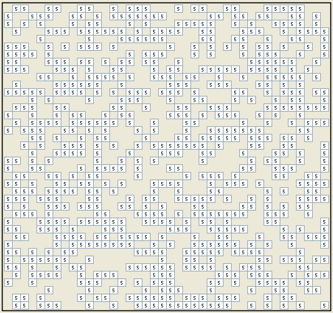
Figure 2: Screenshot of a default grid. The value in the box corresponds to the outcome value provided by the participant.
The participants were 80 undergraduate first year University of New South Wales psychology students (48 females), with an average age of 19.5 years and a range of 18 to 36 years. Participation was in exchange for course credit, plus payment contingent upon choices.
Table 1: Percentage choosing the option predicted by Prospect Theory (Kahneman & Tversky, 1979) to be favoured.
Option Percentage selecting the favoured option Note: * indicates significant difference between description and experience conditions.
The eight choice problems used are shown in first three columns of Table 1. Each problem consisted of two options: an option that probabilistically paid out one of two values versus an alternative option that always paid out a single value. The expected value was always higher for the probabilistic option. The problems were chosen to evenly split between the domains of gain and loss, and also to span a range of probabilistic rarity (5%, 10%, 15%, and 20%). The option predicted by Prospect Theory to be preferred was labelled the “favoured” option and the alternative option was labelled the “non-favoured” option (Kahneman & Tversky, 1979). Specifically, the favoured option was the option containing the rare event when the rare event was desirable (e.g., 14 is a desirable rare event in the option 14 [.15] and 0 [.85]), or the alternative option when the rare event was undesirable (e.g., 0 is an undesirable rare event in the option 4 [.8] and 0 [.2]).
The decision task was the free sampling “money machine” paradigm, similar to the one employed by Hertwig et al. (2004). In the description-based choice condition, two alternative money machines were presented on screen. Each machine was labelled with a description of how that machine allocated points. All of the safe option machines were labelled in the form “100% chance of x”, where x represents the outcome. All of the risky option machines were labelled in the form “y% chance of x, else nothing”, where y represents the probabilistic chance of a non-zero outcome, and x represents the outcome.
In the experience-based choice condition, the two alternative money machines were also presented on screen, but they were labelled only with the letters “A” and “B”, respectively. Each of the machines was associated with a distribution of possible outcomes in accordance with the objective probabilities as shown in Table 1. Samples from each machine were non-random draws from the respective outcome distributions that were selected by an algorithm to maximally match the objective probability with the participants’ experienced distribution, thereby minimising sampling variability.2
In both decision conditions, when the participants were ready to make a one-shot decision, they pressed on a “Play Gamble” button that allowed them to select the machine they preferred to play from. In all cases allocation of safe and risky options to the left and right machines was counterbalanced and the order of the problems was randomised for each participant.
Both the verbal and nonverbal judgment probes asked participants to first enter the number, and specific value, of each outcome paid out by each machine. Contingent on this response, participants were then subsequently asked to provide a probability estimate for each identified outcome. Thus, participants were not asked to make an estimate for an outcome they had not seen, and some participants did not make an estimate for an outcome they had seen (because they had not identified this outcome initially).
The verbal judgment probe asked participants to complete the sentence: “x is paid out by the machine __ percent of the time”, where “x” refers to the outcome. In contrast, the nonverbal judgment probe presented a grid made up of 40x40 small squares, each containing the number “x”, along with the instructions: “Adjust the frequency of x’s in the grid to match the frequency of x paid out by the machine. You can adjust the density of the grid by pressing ‘up’ and/or ‘down’ on the keyboard until x fills the grid according to its frequency”. The default grid showed 50% of the squares, randomly dispersed (Figure 2). Each press of the key increased or decreased the frequency of squares by 1%, randomly over the grid. For the purposes of analysis, the visual display was converted into a percentage after the participant made his or her judgment.
The experiment was a 2 x 2 x 2 within-subjects design and counterbalanced such that participants completed one of the eight problems in each of the eight experimental cells. The three binary independent variables were presentation mode (description or experience), judgment probe type (percentage or grid), and judgment probe time (before or after choice). The two dependent variables were the choice made (favoured or non-favoured option) and the accuracy of judged outcome probabilities (measured as the average absolute difference between experienced3 and judged probabilities).
An on-screen video tutorial explained that the experiment was about making decisions between different alternatives, that the objective of the game was to maximise the amount of points won, and that at the end of the experiment points would be converted into real money according to the conversion rate of 10 points = AUD$1. The tutorial combined written instructions with movements of a ghost player to demonstrate how to play the description- and experience-based decision tasks and correctly answer the verbal and nonverbal judgment probes. Participants were informed that they could sample from each option as often and in any order that they liked. Thus, participants could take samples ranging in size from one to many hundreds. Instructions for the grid probe were: “You will see small versions of the target value randomly superimposed on a square grid. You should adjust the density of the target value on the grid to match the frequency of the target value paid out by the machine.” In order to reduce potential wealth effects, no feedback was given of the points that participants were awarded for their one-shot choice for each problem.
At the completion of the experiment a screen revealed the participant’s total points earned, as well as their corresponding real money conversion. Participants that ended up with negative point scores were treated as though they had scored zero points. Finally, participants were thanked, debriefed, and then paid.
Figure 3: Experienced percentages plotted against judged percentages as a function of presentation mode (description on left panels, experience on right panels) and judgment probe type (verbal percentage in upper panels, nonverbal grid in lower panels). The size of the plotted circles relates the number of identical data points. The solid line depicts the least-square regression lines describing the relation between the experienced and judged probabilities.
Figure 3 plots judged probabilities against experienced probabilities separately for both presentation modes (description vs. experience) and both judgment probe types (percentage vs. grid).4 Inspection of the figure suggests that there is an interaction between presentation mode and judgment probe type. Specifically, it appears that the verbal percentage probe produced better calibrated judgments for those in the Description condition (i.e., estimates closer to the identity line), whereas the non-verbal grid probe produced better calibrated judgments for those in the Experience condition.
We tested this interaction using a mixed model (using the lmer function of R [Bates & Maechler, 2009; R Development Core Team, 2008], as described by Baayen, Davidson, & Bates, 2008, and Bates, 2005). This function is robust when designs are unbalanced, as is the case here as a result of omitted data. The dependent variable was a measure of judgment error: the absolute value of the difference between, on the one hand, the experienced probability of the common event, and, on the other, the normalized judged probability of the common event (i.e., the judged probability of the common event divided by the sum of that and the judged probability of the rare event — the two often did not add to 100). The main predictors were presentation mode, judgment probe type, and their interaction. Problem number (as a nominal variable or factor) was also included as a fixed effect; it accounted for significant variance, but judgment probe time (before vs. after choice) was excluded because it was never significant in any analysis. Participant identity was included as a random effect. The interaction was significant at p = .0042 (as assessed by Markov Chain Monte Carlo sampling). Thus, the magnitude of the difference between participants’ experienced probabilities and their judged probabilities varied depending on whether the information was acquired by description or experience. Examination of the fitted mean errors revealed that participants in the Description conditions were relatively more accurate with the percentage probe than the grid probe (M = 0.98 vs. 6.64, respectively) compared to participants in the Experience conditions (M = 3.22 vs. 5.70, respectively). Further inspection of the two bottom panels of Figure 3 suggests that there is a difference in the slopes of the regression lines between the Description and Experience conditions.
In order to make this directional inference, we regressed an error term (common event judged probability — common event experienced probability) on presentation mode (description vs. experience) for cases where the nonverbal grid judgment probe was used. After removing one outlier, the interaction was significant at p = .0291. A similar analysis for cases where the verbal percentage judgment probe was used was not significant. Thus, the tendency to overestimate rare events and underestimate common events was much stronger in the Description condition, but only when assessed with the nonverbal probe.
The percentage of participants selecting the option predicted by Prospect Theory to be the favoured choice is displayed in Table 1. The difference between Description and Experience conditions falls in the expected direction for six of the eight problems.5 Two of these differences were significant by individual chi-square tests (p’s < .05). Indeed, the odds of selecting the favoured option in the Description condition were more than 1.7 times the odds of selecting the favoured option in the Experience condition. Although indicative, and commonly used in the literature, this rough analysis fails to properly assess the role of presentation mode because it ignores the variance in participants’ experience and judgments.
To test the effect of presentation mode on choice, we used a logistic mixed model, with participant identity as a random effect, and including problem number as a fixed effect (as before). The dependent variable was whether or not the favoured option was selected. The main predictors were presentation mode, judgment probe type, experienced probability and normalized judged probability (as used before). Of these predictors, the only significant effects were of presentation mode (coefficient −.627, z = −3.43, asymptotic p = .0006) and experienced probability (coefficient −.071, z = -2.38, p = .0172). The odds of selecting the favoured option in the Description condition were more than 1.8 times the odds of selecting the favoured option in the Experience condition. Importantly, the effect of normalized judgment was not significant (z = −.90). Thus, the effect of presentation mode on choice is apparently not mediated by its effect on judgment.
Figure 4: The percentage of participants selecting the favoured option in the Description and Experience conditions. The conditionalised data were those trials where the participants’ experienced and (normalised) judged rare event probabilities were both within 10% of the objective rare event probability (see footnote 6). Error bars indicate the standard error of the mean.
In order to show this result graphically, we conditionalised on the subset of data where participants’ experienced and judged distributions were approximately equal to the objective distribution.6 The subset of data comprised of just 28 experience- and 153 description-based decision trials. Thus, the subset did not equally represent all participants, problems and conditions, and, hence, inferential statistics were not conducted. Nevertheless, the retained data do serve to visually represent the major finding of our regression analysis. Namely, as shown in Figure 4, even within the subset of data without sampling or judgment errors, there remains a gap between description- and experienced-based choices.
The current study attempted to take a representational perspective in explaining the observation of a gap between description- and experienced-based patterns of choice. The first aim was to examine whether there exists representational bias, that is, an encoding distortion of the outcome distribution prior to choice. To that end, we asked participants to judge each problem’s outcome distribution using either a verbal or nonverbal probe.
When participants made their judgment using a nonverbal probe — adjusting the density of a large grid to correspond to the relative probability of each outcome — absolute judgment accuracy in the Description and Experience conditions was approximately equivalent. This result is particularly surprising because it implies that decision makers are equally able to nonverbally represent a non-explicit, gist impression constructed from sequential sampling and a numerical percentage explicitly presented. Of course, this is not to say that judgments were particularly accurate: they were not; participants in both groups displayed a tendency to underestimate common events and overestimate rare events. This observation replicates Gottlieb et al.’s (2007) intriguing finding that percentages are distorted when transformed into nonverbal estimates. The current study extends this observation to a free sampling design where participants decided the size of their samples. Admittedly, it is possible that at least some of this bias is due to an anchoring effect at the probe-density starting point (50%). What is perhaps more interesting, and not explainable in terms of anchoring, is the fact that the distortion, this tendency to underestimate common events and overestimate rare events, was much greater for those in the Description conditions than those in the Experience conditions.
When participants made their judgment using a verbal probe — entering a number to correspond to the relative probability of each outcome — absolute judgment accuracy was greater in the Description conditions. Contrary to some previous research, there was little evidence that participants overestimated small probabilities and underestimated large probabilities (Barron & Yechiam, 2009; Hau et al., 2008). In fact, accuracy in both conditions was fairly high, which replicates some other studies that have asked for probability judgments (Fox & Hadar, 2006; Gottlieb et al., 2007; Ungemach et al., 2009), and were superior to those achieved by participants making judgments via the nonverbal grid probe.
The greater absolute judgment accuracy observed when using the verbal probe may lead some to the conclusion that this type of probe should be preferred when assessing representations of outcome distributions We have three cautions. First, accuracy when using the verbal probe in the Description condition depended only on memory, not judgment, and is therefore inflated. Second, the nonverbal grid task was, on average, prone to greater variability because of the potential for super- or sub-additivity. Specifically, because one grid was presented for each outcome identified, participants’ summed judgments for the outcome probabilities for each option often deviated from 100%. Super- and sub-additivity did not occur when using the percentage probe because participants could easily add up their estimates and ensure that they totalled 100%. Third, even if decision-makers can interpret and numerically report the content of their mental representations when explicitly probed by a verbal probe, if this is not the actual representation and information used to make the decision, then such (albeit accurate) information is non-diagnostic in the pursuit of understanding experience-based choice.
What then are we to conclude about nonverbal judgment probes? Despite producing less accurate results overall, they uniquely discriminate between description- and experience-based formats of information acquisition. Nonverbal judgment probes may therefore permit greater sensitivity to presentation mode when gauging mental representations. Potentially, this is because representations of outcome distributions are themselves nonverbal (Dehaene et al., 1998).
The second aim was to examine whether representational biases constitute, in addition to sampling bias, a major cause of the choice gap between description and experience choice formats. As described above, there does appear to be a representational bias, at least when probed nonverbally, and this bias is stronger when information is acquired by description. Assuming choices are made based on these differentially distorted outcome distributions, representational biases may be sufficient to cause subsequent differences in choice.
To begin, we again found a disparity in the patterns of choice made to identical problems depending on whether they were presented by description or experience (Hertwig et al., 2004; Weber et al., 2004). The size of the gap observed in our data, 14.4 percentage points, is relatively small when compared to previous free sampling DfE paradigm studies (e.g., 36 percentage points in Hertwig et al., 2004). This is probably due to the relatively large amount of samples taken by our participants (median of 28, compared to 15 in Hertwig, et al., 2004) coupled with our manipulation for sample outcomes to track the objective probabilities as closely as possible (see Footnote 2).
Even after accounting for sampling bias and judgment distortions, however, the mode by which information was acquired — by description or from experience — remained significant. The differential distortions observed in judged outcome distributions across presentation mode did not mediate the choice gap between description- and experience-based choices. Importantly then, the choice gap appears to be being driven by something over and above both sampling bias and judgment distortions. This finding supports the work of those that have obliged participants to sample until they have observed outcomes matching exactly or nearly exactly the objective outcome distribution (Hau et al., 2008; Jessup, Bishara, & Busemeyer, 2008; Ungemach et al., 2009).
How can we explain the remarkable conclusion that participants’ own estimate of the outcome distribution does not mediate their subsequent choice? It may be the case that choices are made separately from judgment of the outcome distributions. Recently it has been noted that in many situations, both inside and the lab and out, people’s choice behaviour is at odds with their judgment (Barron & Yechiam, 2009). For example, immediately following a suicide bombing, people believe the risk decreases but at the same time exhibit more cautious behaviour. Thus, choice may not be made using representations of the outcome distributions at all. Decision field theory, for example, models choice processes as the gradual change of preference between options and makes no reference to a mental representation of each option’s outcome distribution (Busemeyer & Townsend, 1993). This conclusion has implications for the development of models of choice. Specifically, our results suggest that models that incorporate two stages, one at the level of representation and one at the level of choice, may be unnecessary when it comes to predicting experienced-based choice. For example, one of the leading two-stage choice models — cumulative prospect theory (Fox & Tversky, 1998; Tversky & Fox, 1995) — fares no better at explaining our data when based on judged, compared to experienced, outcome distributions (Appendix). This result echoes the finding of Hau et al. (footnote 2, 2008). Our conclusion also seems to be consistent with the findings from a recent choice prediction competition. Whereas all models submitted to predict description-based choices assumed that outcomes were weighted by probabilities, the majority of models submitted to predict experience-based choices were such that “the concept ‘probability’ did not play an important role” (Erev et al., 2010).
With regard to the two primary choice gap explanations — statistical or psychological — the current data lend support to the latter account. That is, that there exist true differences in the choice mechanics used to make experience-based decisions that are over and above the effects of biased samples and judgment errors. What else could be driving the gap? Hertwig et al. (2004) demonstrated that recency, the tendency to rely more heavily on more recently observed outcomes, was another influence on experienced-based choice and hence the gap. In our data, however, we observed no difference in success when predicting choice from the mean value of the first versus second half of observed outcomes (56.2% versus 60.5%, respectively, t(560) = −1.026, n.s.). Our interpretation is that the gap derives from a probabilistic focus in the description format and a non-probabilistic focus in the experience format. Indeed, Rottenstreinch and Kivetz (2006) argue that non-probabilistic thinking is more likely in situations where people partially control events and when there is relatively low salience of probabilistic cues. If Rottenstreinch and Kivetz’s interpretation is correct, the experience format in which probabilities are never explicitly mentioned is more likely to yield non-probabilistic thinking than the description format in which probabilities are clearly presented. Moreover, evidence from outside the lab also suggests that executives’ decision-making rarely explicitly considers outcome probability (Jeske & Werner, 2008). We feel that the distinction between a probabilistic and non-probabilistic focus during choice is an interesting one for further research to pursue.
Baayen, R. H., Davidson, D. J., & Bates, D. M. (2008). Mixed-effect modeling with crossed random effects for subjects and items. Journal of Memory and Language, 59, 390–412.
Barron, G., & Yechiam, E. (2009). The coexistence of overestimation and underweighting of rare events and the contingent recency effect. Judgment and Decision Making, 4, 447–460.
Bates, D. (2005). Fitting linear mixed models in R. R news, 5, 27–30. http://journal.r-project.org.
Bates, D. & Maechler, M. (2009). lme4: Linear mixed-effects models using S4 classes. R package version 0.999375–32, http://CRAN.R-project.org/package=lme4.
Bonner, C., & Newell, B. R. (2008). How to make a risk seem riskier: The ratio bias versus construal level theory. Judgment and Decision Making, 3, 411–416.
Busemeyer, J. R., & Townsend, J. T. (1993). Decision Field Theory: A dynamic cognition approach to decision making. Psychological Review, 100, 432–459.
Camilleri, A. R., & Newell, B. R. (in preparation). The description-experience ’gap’: Psychological or statistical phenomenon? The University of New South Wales.
Dehaene, S., Dehaene-Lambertz, G., & Cohen, L. (1998). Abstract representations of numbers in the animal and human brain. Trends in Neurosciences, 21, 355–361.
Erev, I., Ert, E., Roth, A. E., Haruvy, E., Herzog, S., Hau, R., Hertwig, R., Stewart, T., & Lebiere, C. (2010). A choice prediction competition, for choices from experience and from description. Journal of Behavioral Decision Making, 23, 15–47.
Fox, C. R., & Hadar, L. (2006). “Decisions from experience” = sampling error + prospect theory: Reconsidering Hertwig, Barron, Weber & Erev (2004). Judgment and Decision Making, 1, 159–161.
Fox, C. R., & Tversky, A. (1998). A belief-based account of decision under uncertainty. Management Science, 44, 879–895.
Gigerenzer, G., & Hoffrage, U. (1995). How to improve Bayesian reasoning without instruction: Frequency formats. Psychological Review, 102, 684–704.
Gottlieb, D. A., Weiss, T., & Chapman, G. B. (2007). The format in which uncertainty information is presented affects decision biases. Psychological Science, 18, 240–246.
Hadar, L., & Fox, C. R. (2009). Information asymmetry in decision from description versus decision from experience. Judgment and Decision Making, 4, 317–325.
Hau, R., Pleskac, T. J., & Hertwig, R. (2010). Decisions from experience and statistical probabilities: Why they trigger different choices than a priori probabilities? Journal of Behavioral Decision Making, 23, 48–68.
Hau, R., Pleskac, T. J., Kiefer, J., & Hertwig, R. (2008). The description-experience gap in risky choice: The role of sample size and experienced probabilities. Journal of Behavioral Decision Making, 21, 1–26.
Hertwig, R., Barron, G., Weber, E. U., & Erev, I. (2004). Decisions from experience and the effect of rare events in risky choice. Psychological Science, 15, 534–539.
Hertwig, R., & Erev, I. (2009). The description-experience gap in risky choice. Trends in Cognitive Sciences, 13, 517–523.
Hertwig, R., & Pleskac, T. J. (2008). The game of life: How small samples render choice simpler. In N. Charter & M. Oaksford (Eds.), The probabilistic mind: Prospects for rational models of cognition (pp. 209–236). Oxford: Oxford University Press.
Jeske, K.-J., & Werner, U. (2008). Impacts on decision making of executives — Probabilities versus outcomes. Journal of Neuroscience, Psychology, and Economics - Research, 1, 49–65.
Jessup, R. K., Bishara, A. J., & Busemeyer, J. R. (2008). Feedback produces divergence from Prospect Theory in descriptive choice. Psychological Science, 19, 1015–1022.
Kahneman, D., & Tversky, A. (1979). Prospect theory: An analysis of decision under risk. Econometrica, 47, 263–291.
Kareev, Y. (1995). Through a narrow window: Working memory capacity and the detection of covariation. Cognition, 56, 263–269.
Kareev, Y. (2000). Seven (indeed, plus or minus two) and the detection of correlations. Psychological Review, 107, 397–402.
R Development Core Team (2008). R: A language and environment for statistical computing. R Foundation for Statistical Computing, Vienna, Austria. ISBN 3–900051–07–0, http://www.R-project.org.
Rakow, T., Demes, K. A., & Newell, B. R. (2008). Biased samples not mode of presentation: Re-examining the apparent underweighting of rare events in experience-based choice. Organizational Behavior and Human Decision Processes, 106, 168–179.
Rakow, T., & Newell, B. R. (2010). Degrees of uncertainty: An overview and framework for future research on experience-based choice. Journal of Behavioral Decision Making, 23, 1–14.
Rottenstreich, Y., & Kivetz, R. (2006). On decision making without likelihood judgment. Organizational Behavior and Human Decision Processes, 101, 74–88.
Simon, H. A. (1990). Invariants of human behavior. Annual Review of Psychology, 41, 1–19.
Todd, P. M., & Gigerenzer, G. (2000). Précis of simple heuristics that make us smart. Behavior and Brain Sciences, 23, 727–780.
Tversky, A., & Fox, C. R. (1995). Weighing risk and uncertainty. Psychological Review, 102, 269–283.
Tversky, A., & Kahneman, D. (1992). Advances in prospect theory: Cumulative representation of uncertainty. Journal of Risk and Uncertainty, 5, 297–323.
Ungemach, C., Chater, N., & Stewart, N. (2009). Are probabilities overweighted or underweighted, when rare outcomes are experienced (rarely)? Psychological Science, 20, 473–479.
Weber, E. U., Shafir, S., & Blais, A.-R. (2004). Predicting risk sensitivity in humans and lower animals: Risk as variance or coefficient of variation. Psychological Review, 111, 430–445.
One of the most successful models in the area of description-based choice is prospect theory (Tversky & Kahneman, 1992). According to prospect theory, decision makers calculate a “value” for each alternative by multiplying the utility value of the outcome by a decision weight. Crucially, the value and decision weight functions are nonlinear. For example, the decision weight function implies that people overweight low percentages and underweight moderate and high percentages. Particularly germane in light of the current experiment, the two-stage model of cumulative prospect theory (CPT) applies the decision weight function adjustment to the decision maker’s judged outcome percentage, as opposed to the objective or experienced percentage (Fox & Tversky, 1998; Tversky & Fox, 1995).
We used CPT to predict choices as a function of objective, experienced, as well as raw judged probabilities for the non-zero event (see Hau et al., 2008 for details). We fitted the data to two versions of cumulative PT: one based on parameters estimated from description-based choice (Tversky & Kahneman, 1992), and one based on parameters estimated from experience-based choice (Hau et al., 2008).
As shown in Table 2, each version of the PT model did relatively poorly. Unsurprisingly, description-based choices were better predicted with parameters estimated from described choices tasks, and experienced-based choices were better predicted with parameters estimated from experienced choices. In the Experience conditions, on average, there was little difference in prediction accuracy between judged or experienced percentages, but both did better than objective percentages.
Table 2: Percentage of choices correctly predicted by Cumulative Prospect Theory when fitted with parameters estimated for description (Tversky & Kahneman, 1992) and experience-based choice (Hau et al., 2008).
Fitted with Tversky and Kahneman (1992) estimated parameters % choices correctly predicted Description Experience Fitted with Hau et al. (2008) estimated parameters % choices correctly predicted Description Experience Note: Objective percentages refer to the underlying problem outcome distribution. Experienced percentages refer to the outcome distribution observed during sampling. Judged percentages refer to the estimated outcome distribution.
This document was translated from LATEX by HEVEA.