Relativistic financial decisions: Context effects on retirement saving and investment risk preferences

Ivo Vlaev¹ and Nick Chater
Department of Psychology
University College London, Neil Stewart
Department of Psychology
University of Warwick

Judgment and Decision Making, vol. 2, no. 5, October 2007, pp. 292-311

Abstract

We report a study of the effects the choice set on financial decision making related to retirement savings and risky investment. The participants were presented with either a full range of choice options or a limited subset of the feasible options. The choices of saving and risk are affected by the position of each option in the range of presented options. This result demonstrated that the range of the options offered as possible saving rates and levels of investment risk influences decisions about saving and risk. The study was conducted on a sample of working people, and we controlled whether the participants can financially afford in their real life the decisions taken in the test. In addition, various measures of risk aversion did not account for the risk taken in each condition. Surprisingly, only the simplest and most direct risk preference measure was a significant predictor of the responses within a particular choice set context, although the actual choices were still very much influenced by the range. Thus, the results reported here suggest that financial judgments and choices are relative, which corroborates, in an important practical domain, previous related work with abstract gambles and hypothetical risky investments.

Keywords: context effects, decision making, judgment, investment risk, saving.

1 Introduction

This article presents a study that investigated how far simple, and practically relevant, modifications in the decision making context can affect how people make financial decisions related to retirement savings and investment. Specifically, we aim, using a realistic setting, to make a suggestive replication of a new and powerful context effect - prospect relativity (Stewart, Chater, Stott, & Reimers, 2003), in an important practical domain.

In this article, we present a study that investigates the effects of the framing and presentation of financial information when asking people to express their preferences in relation to different retirement savings and investment scenarios. The experimental design and method are based on the recent discovery of a substantial dependence of human preferences on the set of options they are presented with. This phenomenon was termed prospect relativity and indicates a lack of stable underlying preference function (Stewart et al., 2003). This finding, which we describe in more detail below, is striking illustration of the view that preferences are often constructed, on the fly, rather being a stable basis for decision making (Slovic, 1995).

A theoretically important question is how far these effects transfer from abstract low-stakes gambles to major financial decisions that could significantly affect long-term well-being. If we observe such transfer to realistic financial decisions, then this would have practical significance for marketing, sales, and provision of advice in the financial services industry. Our goal was to investigate how far individual variation in saving and risk preferences is stable across different realistic decision contexts.

1.1 Theoretical background

In search of such realistic psychological foundations for descriptive decision theory, Stewart et al. (2003) considered whether context effects observed in psychophysics might transfer to risky decision making. Specifically, Stewart et al. found that the set of options, from which an option was selected, almost completely determined the choice. They demonstrated this effect in selection of a risky prospect and in certainty equivalent estimation task (the amount of money for certain that is worth the same to the person as a single chance to play the prospect). Similarly, the selection of a preferred option from a set of prospects was strongly influenced by the prospects available. More recently, Stewart, Chater, and Brown (2006) developed a model of risky choice, decision by sampling, which assumes relative judgments and provides one explanation for the results in Stewart et al. (2003).

The cognitive claim that Stewart et al. (2003) advance is that people are often unable to represent absolute magnitudes, whether psychophysical or abstract (including a choice option's attributes like utilities, payoffs, and probabilities). That is, when people represent a magnitude, they can do so only on the basis of whether it is larger or smaller than other magnitudes retrieved from memory or observed in the environment. If people cannot represent the absolute value of magnitudes on any cardinal scale, and the subjectively judged utility of an option is determined by its relationship to comparison options, then judgments will be strongly affected, or even determined, by the context.

The core evidence for this claim comes from the study of the perception of the intensity of basic psychophysical magnitudes such as the brightness of a light or the loudness of a sound. Much traditional research in psychophysics has assumed the existence of some cardinal internal scale of intensities, onto which physical stimulation must somehow be mapped; and there has been consequent debate concerning the nature of this mapping (e.g., whether it is logarithmic, as argued by Fechner, 1966; or a power law, as argued by Stevens, 1957). But more recent theory (reviewed and analysed in Laming, 1997) suggests a different point of view - that the very idea of an internal scale is questionable. In particular, Laming (1997) has shown that empirical data in line with Stevens' power law (relating psychophysical variables and free numerical judgments) can arise without assuming any representation of absolute information. In addition, Stewart, Brown, and Chater (2005) demonstrated that a wide range of data from the psychophysical task of absolute magnitude identification can be captured by a model which has no absolute scales, and relies entirely on local comparisons between recent stimuli.

A particularly telling example supporting this viewpoint is an elegant experiment conducted by Garner (1954), who asked participants to judge whether tones were more or less than half as loud as a 90 dB reference loudness. Participants' judgments were entirely determined by the range of tones played to them. There were three groups of participants who received tones in three different ranges respectively. Participants who heard tones in the range 55-65 dB had a half-loudness point (i.e., where their judgments were "more than half as loud" 50% of the time and "less than half as loud" 50% of the time), of about 60 dB. Another group, who received tones in the range 65-75 dB had a half-loudness point of about 70 dB. A final group, who heard tones in the range 75-85 dB, had a half-loudness point of about 80 dB. Garner's experiment indicates, therefore, that people find it difficult to judge the absolute intensity of the sound (or what it means for one sound to be half as intense as another). Instead, it seems that people adjust their responses depending on the presented sound intensities from which they are asked to choose, which demonstrates that the context is very overwhelming when it is present.

Other examples of similar context effects abound in psychophysics (see Stewart et al. 2003; Stewart, Chater, & Brown, 2006; for a more extensive review of studies showing that perceptual judgments of stimuli varying along a single psychological continuum are strongly influenced by the preceding material), which are consistent with participants making perceptual judgments on the basis of relative, rather than absolute magnitude information.

Here we have digressed briefly into psychophysics, in order to make it explicit how we apply the resulting conclusion to a decision-making context. Note, though, that the parallel between the two domains, psychophysics and economic decision making, is relatively close. After all, just as perceptual theorists traditionally assumed that people have internal scales for the representation of loudness and brightness, so a traditional psychological or economic picture of an agent assumes that the agent must have internal scales for the representation of the utility and the probability (perhaps distorted as shown by Kahneman & Tversky, 1979) of various outcomes. Without some type of scale for utility or probability, the model of the economic actor (or any decision-making agent in general) would look very different.

1.2 Previous results

One prediction based on such model is that the attributes of the previously or currently seen risky prospects influence the decisions in the current prospect. Stewart et al. (2003) argued for the existence of what they called prospect relativity: that the perceived value of a risky prospect (e.g., "p chance of x") is relative to other prospects with which it is presented. Note that Stewart et al. studied peoples' perception of utilities in individual decision making tasks in gambling situations. The prediction, based on the psychophysical studies described above, is that the option set (i.e., the context) will affect peoples' choices because there is no fixed internal scale according to which people make their judgements of the values of certain options. The results demonstrated a powerful context effect in judging the value of different risky prospects - the set of options offered as potential certainty equivalents for simple prospects was shown to have a large effect on the certainty equivalents selected. For example, when during judging the value of a 50% chance of winning £200 people have options of £40, £50, £60, and £70, the most popular choice is £60 and then second choice is £50. When people have options of £90, £100, £110, £120 pounds, the most popular choice is £100, and then second choice is £110. So the set of alternatives affected valuation by a factor of (almost) 2. This effect was replicated despite monetary incentives designed to encourage participants to deliver accurate and truthful certainty equivalents. In another experiment, the set from which a simple prospect was selected was also shown to have a large effect on the prospect that was chosen.

Vlaev and Chater (2006) discovered similar results in a very different context, where people play the strategic games based on Prisoner's Dilemma, indicating the generality of this effect. In particular, this study showed that the so-called "cooperativeness" of the previously played games influence choices and predictions in the current game, which suggests that games are not considered independently. These effects involved a perceptual contrast of the present game with preceding games, depending on the range and the rank of their cooperativeness.

Finally, Vlaev, Chater, and Stewart (2007) report three studies, in which methodologies from psychophysics (which were similar to the methods used by Stewart et al., 2003) were adapted to investigate context effects on individual financial decision making under risk. The aim was to determine how the range and the rank of the options offered as saving amounts and levels of investment risk influence people's decisions about these variables. In the range manipulation, participants were presented with either a full range of choice options or a limited subset, while in the rank manipulation they were presented with a skewed set of feasible options. The results showed that choices are affected by the position of each option in the range and the rank of presented options, which suggests that judgments and choices are relative.

Effects of the type presented above suggest that people's expressed (or revealed) risk preferences are not absolute, but are, to some degree at least, relative to the range of available options (see Stewart, Chater, & Brown, 2006, for model of risky choice that assumes relative judgments only). A plausible account of the context effects caused by the range of options is the range-frequency theory proposed by Parducci (1965, 1995). Parducci found that the neutral point of the judgment scale did not correspond to the mean of the contextual events, contrary to (then popular) adaptation level theory (Helson, 1964), but rather to a compromise between the midpoint (defined by the range) and median (depending on the skew) of the distribution of contextual events. For example, satisfaction judgements are different between two distributions of life events, which have different skew and identical means. The range principle reflects tendency to judge an event relative to its position within the range of stimuli on the specified dimension of judgment, while the frequency principle reflects a tendency to judge an event relative to its rank within the immediate context. The subjective value given to an attribute is a function of its position within the overall range of attributes, and its rank. Thus, this model implies that attributes are judged purely in relation to one another and their subjective value is independent of their absolute value. Range-frequency theory has already been used to account for context effects in decision making under risk. Birnbaum (1992), Stewart et al. (2003), Vlaev and Chater (2006), and Vlaev, Chater, and Stewart (2007) found their data to be consistent with the theory.

Similar effects in a more practical domain were shown by Benartzi and Thaler (2002) who offered the respondents a choice between retirement investment options with varying ranges of expected future income (e.g., chose between $900 monthly pension for sure and a 50/50 chance to get either $1,100 per month or $800 per month after retirement). When the range of investment programs comprised three options varying from low risk to high risk, the investors selected the middle options significantly more often irrespectively of their absolute risk level (e.g., the same option was judged as the least attractive one when positioned at the top of the range, but also perceived as the most attractive one when in the middle of the range).

Note that these relativistic patterns may also reflect a more general tendency to prefer central options that is seen when choosing amongst identical options (e.g., if people cannot differentiate between the presented options due to ignorance, indifference, etc.), which may be an example of the compromise effect (also called extremeness aversion; see Simonson & Tversky, 1992). Indeed in the compromise effect (e.g., Simonson, 1989), an option that represents a compromise between two alternatives may be preferred over the alternatives, even though the alternatives are preferred over this option in a pairwise binary choice.

In this article, we present a suggestive extension of our previous work (Stewart et al. 2003; Vlaev & Chater, 2006; Vlaev, Chater, & Stewart, 2007) to an important practical domain (similarly to Benartzi & Thaler, 2002). In particular, we aimed to replicate the prospect relativity principle to more realistic financial decision making scenarios. The results we present here suggest that, when people make financial decisions, the attractiveness of the choice options significantly depends on the other available options.

Table 1: Figures for saved amount (£), investment risk (%), and retirement age in the three conditions of the experiment.

	Low Range			High Range
Save	Risk	Retire	Save	Risk	Retire	Save	Risk	Retire
500	0	48	500	0	48
1,000	10	50	1,000	10	50
1,500	20	52	1,500	20	52
2,000	30	54	2,000	30	54
2,500	40	56	2,500	40	56
3,000	50	58	3,000	50	58	3,000	50	58
3,500	60	60				3,500	60	60
4,000	70	62				4,000	70	62
4,500	80	64				4,500	80	64
5,000	90	66				5,000	90	66
5,500	100	68				5,500	100	68

2 Experiment

2.1 Prospect relativity principle and realistic financial decision scenarios

Thus the main goal of this experimental study was to make a provisional estimate of the degree to which the kinds of effects that are revealed by Stewart et al. (2003) could also be applicable to real financial decisions. Our study builds on, and is similar to, the study by Vlaev, Chater, and Stewart (2007). The domain used here, and also by Vlaev, Chater, and Stewart, was saving and investment for retirement, because it is an issue having serious social relevance at the moment. We currently live in a financial environment in which aging population and younger consumers are increasingly expected to take command of their own pension and investment decisions. Therefore, the following two key issues arise: How does the range of options people choose between affect the level of pension investment they choose? How does the range of options from which people choose affect the level of risk they accept with that investment?

This experiment followed logic similar to the decision experiments reported by Stewart et al. (2003) and Vlaev, Chater, and Stewart (2007), which were in turn inspired by Garner's (1954) loudness judgment experiment. In various questions, the participants in our study were asked to select among a predefined set of values related to five variables: (a) the desired percentage of the annual income that will be saved for retirement, (b) the investment risk expressed as the percentage of the saving that will be invested in risky assets, (c) retirement age, (d) expected retirement income, and (e) possible variability of the retirement income.

There was a control condition, in which the participants had to freely decide the value of each one of these variables selecting from the full range of options. In two context conditions, participants were asked to select these values from sub-ranges of the set of options offered by the experimenter in the full range condition. Thus, there were three between-participant conditions in the experiment presented here, i.e., with separate groups for the full range, low range, and high range conditions. In the full range condition, all options were presented. In the two other conditions, the choice of prospects was limited to either the first or second half of the prospects available in the free choice condition, so that the participant in the high range condition were presented with a range of values the lowest of which coincides with the highest option in the low context condition.

In the full range condition for saving, the options were presented in monetary terms and varied from £500 to £5,500 increasing with £500 between the options; so there were eleven options to choose among, while the low range condition spanned from £500 to £3,000 and the high range condition was from £3,000 to £5,500. The same design was applied for the risk variable. The choice option values in the full range condition for investment risk varied from 0% to 100% and were increasing with 10% between the options. For retirement age the values varied from 48 to 68 increasing with 2 years. Table 1 presents the values for savings, risk, and retirement age, in the three conditions. For the retirement income and its variability, the values were different for every question depending on the combination of saved amount, investment risk, and retirement age.

Note that, for risk, it is natural to assume that people anchor the possible percentage of their retirement savings that can be invested in risky assets to be between on 0% and 100% (i.e., people cannot have negative savings, or invest more than 100% of their savings because the use of leverage, like borrowing for example, in retirement accounts is restricted by regulation). For the range of possible savings values, it is equally easy to imagine that the lower bound is zero, while the upper bound depends on many factors such as, for example, legal requirements, cost of living, etc. We fixed the maximum possible savings range across all conditions at £5,500, which is 22% of the average salary in UK at the time (£25,000), because 22% approximates the upper bound for the retirement savings rate in UK due to legal and tax restrictions. The team of professional actuaries who monitored our research project suggested 22% as the practically relevant upper bound.

Figure 1: Predictions in terms of cumulative frequencies of choices, which would be expected, if people have (a) fixed, and (b) relative, level of risk aversion.

2.2 Hypotheses

Our prediction was that, if a participant is not influenced by the set of options, then his or her choice of each value in the high and low range conditions should be independent of the other values in the set and the chosen values should be the nearest to his or her free choice. It is helpful to consider the predictions (represented in terms of cumulative frequencies of choices), that would be expected if people have a fixed and absolute level of preference for saving, (or any other preferences), which they use to make their choices. If we suppose that, where the full set of choices is available, people make each choice roughly equally, then, the cumulative frequency is an increasing linear function of saving rate, shown as a straight line in the upper part of Figure 1a. If the choice set is restricted to the lower saving options only, then all the participants who would, in the full context condition, have chosen one of the higher saving options, were they still available, should instead choose the highest available option. The choices of all other participants should be unchanged. (This follows on the assumption that people choose according to a fixed absolute saving/consumption preference, and hence the availability of non-preferred options should not affect their choices). Thus, the cumulative frequency function should, in the lower saving condition, follow the linear function of the full condition and all remaining participants should choose the highest available option, so that this point goes directly to 1. Similarly, in the case where only the upper range of options is available, the cumulative frequency is clearly at 0 for all the non-available options. If people's judgments are absolute, then participants who would otherwise have chosen the low saving options that are now not available will choose the lowest of the available high options. Specifically, the cumulative frequency should jump directly to the linear function level appropriate in the full range condition and, as other choices in the high range should be unaffected by the presence or absence of non-preferred lower options, the function should then follow the linear function of the full context condition thereafter.

By contrast, the lower part of Figure 1b shows the predictions from the extreme opposite assumption: instead of people choosing saving levels on the basis of fixed, absolute saving (consumption) preferences, they assess saving purely in relative terms. If this is correct, then the pattern of response should have the same distribution, whether the responses are distributed across the full context, or just the lower and upper context. So, if we assume that response is even in the full context condition (and hence that the cumulative probability function is linear), then in the lower and upper contexts, the cumulative distribution should also be linear, but compressed over a smaller number of choice options (i.e., with an increased slope).

We also conducted the following statistical comparison between the high range and low range conditions in order to test furthermore whether the context (range of options) had a significant effect on the choices. We compared the lowest option in the high range, against the sum of all the items in the low range, except the highest item (i.e., every option in the low range, which was missing in the high range). In other words, we compared whether the lowest option in the high range condition was significantly lower than the proportion of times the options below it were selected in the low range condition. Conversely, we compared the highest option in the low range, against the sum of the options in the high range, except the lowest option. In either direction (and we tested both directions), if the latter is bigger, we have a prospect relativity effect (or at least, a rational choice model will fail to predict this result) and we can conclude that this result should be due to the effects of the choice set in the high range and low range condition respectively. The logic behind this analysis is that people who do not select the highest item in the low range condition should definitely select the lowest item in the high range condition. So the former ought to be less numerous than the latter. This is because their true preferences should be within the options lower than the highest item in the low range condition. In other words, the reason we are missing the highest item in the low/high range, is that we do not know what proportion of the people selecting this option want to select options above/below it, but they do not have the opportunity in the low/high range. Alternatively, if participants' responses are solely determined by the set of options presented to them, then the distribution of responses across options should be identical for both the low and the high range conditions.

2.3 Method

2.3.1 Participants

We sent the materials (the financial affordability questionnaire and the savings and investment questionnaire) by post to a population of working individuals, as this population is typically not able to attend laboratory sessions. We sent out the questionnaire to 600 people, and received 64 completed questionnaires. These respondents were typical of the demographics in the geographical area and selected from a big subject pool of people who expressed desire to participate. Participants who completed their questionnaires were paid £10 for their participation (received as a check after they have returned the answer sheet). There were 24 men with mean age 36.5 and 40 women with mean age 37. The Low Range Condition had 20 participants: 7 men (mean age 37) and 13 women (mean age 38); the Free Choice Condition had 21 participants: 9 men (mean age 33) and 12 women (mean age 36); and the High Range Condition had 23 participants: 8 men (mean age 40) and 15 women (mean age 36).

Table 2: A question in the free choice condition, in which the participants were asked to choose their preferred level of investment risk by selecting one of the rows in the table below. In this format the key variable is in the first column of the table, while the other columns are showing the effects on the other three variables (minimum, average, and maximum retirement income).

Now assume that you decided to retire at 65 and to save £3000 per year in order to provide for your retirement income. The following options offer different ranges of retirement income depending on the percentage of your savings invested in the High Risk asset, and you can see in the table the effects on the expected average retirement income and its variability (minimum and maximum). There is such variability of your expected retirement income because when you invest in the High Risk asset your income partially depends on the performance of the market and the economy in general, which might vary over time. Note that the precise amount of your pension is unpredictable, because of possible variation in investment performance, but it is very likely (more than 95% chance) that it will be between (i.e., cannot get below and above) the minimum and the maximum values indicated in the table below. For instance, if you invest 50% per year in the High Risk asset (see the table below), then it is very likely (95 percent chance) that your annual retirement income will be more than £3,250 and less than £5,000, and on average (50 percent chance) you can get more than £4,500. Now please select how much to invest in the High Risk asset.

	Retirement Income
	Minimum	Average	Maximum
0 %	3,500	3,500	4,000
10 %	3,450	3,700	4,200
20 %	3,400	3,900	4,400
30 %	3,350	4,100	4,600
40 %	3,300	4,300	4,800
50 %	3,250	4,500	5,000
60 %	3,200	4,700	5,200
70 %	3,150	4,900	5,500
80 %	3,100	5,000	5,800
90 %	3,050	5,100	6,100
100 %	3,000	5,200	6,500

2.3.2 Design

The experimental design had two main elements. One was the specific financial design of the prospect relativity test and the second was the design of the realistic practical setting that aimed to improve the real-world validity of the test.

Prospect relativity test: The questions in the prospect relativity test were formulated as long-term saving/investment decision tasks related to retirement income provision. The participants had to make decisions about five key variables. These variables were the saved proportion of the current income, the risk of the investment expressed as the proportion invested in risky assets², the retirement age, the desired income after retirement, and the preferred variability of this income (we explained that such variability is due to favourable and respectively unfavourable economics conditions).

The experimental materials were designed as 10 independent hypothetical questions, in which we varied each of the five key variables. However five of the questions focused only on savings while the other five questions focused only on risk, and some questions showed how changing savings or risk would affect another variable or set of variables. For example, how changing the investment risk can affect the projected retirement income and its variability - with higher risk offering higher expected income on average, but also wider spread of the possible values.³ As an example, Table 2 presents a question in the free choice condition, in which the participants were asked to choose their preferred level of investment risk by selecting one of the rows in the table (note that in this format the key choice variable is in the first column of the table while the other columns are showing the effects on the other variables like the minimum, average, and maximum retirement income⁴).

The future distribution (risk) of the investment in risky assets is calculated as follows. Assuming a variable annual interest rate with mean m and standard deviation s, the expected return on an n-year investment is log normally distributed with mean mⁿ and standard deviation s = m²ⁿ (((s²/m²) +1)ⁿ⁺¹). We also assumed that an annuity that provides 1/14th of the lump sum saved each year is purchased, which is a typical figure used in the UK financial services industry. We created test materials for three different age groups, namely, 30, 40, and 50. We sent the identical test materials to respondents who are plus or minus 5 years around each age group (e.g., the financial options calculated for somebody who is 30, were also sent to all respondents between 25 and 35 yrs old). Thus the projected retirement income was calculated for three time horizons: after 35, 25, and 15 years of investment respectively.

Here is a detailed description of each question and its purpose (the questions are grouped by the key variable that participants are asked to select - savings or investment risk). Appendix A presents all questions in an example questionnaire designed for a person who is around 40 years old.

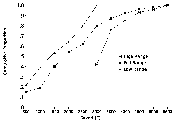
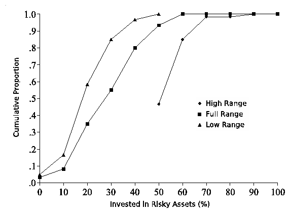
Saving questions There were five questions asking people to choose between savings options presented in monetary terms.

Choose how much to save without information about other variables.

Choose how much to save and see expected retirement income.

Choose how much to save and trade it off with retiring at different age and see the expected retirement income.

Choose how much to save and see the retirement income and its minimum and maximum variability happening because assume that 50% of the savings are invested in the High Risk asset.

Choose how much to save and take different levels of risk starting from low savings and investment risk and then increase both in parallel.

Risk questions. Next are the five questions asking people to choose levels of risk formulated as percentage of saving invested in the High Risk asset:

Choose how much to invest without information about other variables.

Choose how much to invest and see expected retirement income and its variability.

Choose how much to invest and trade-off it with retiring at different age and see the expected retirement income and its variability.

Choose how much to invest and trade-off it with amount to be saved (increasing investment corresponding to decreasing savings) and see the retirement income and its variability.

Choose between levels of variability of the retirement income. Variability reflects different investment strategies and is increasing with the income (higher variability corresponds to higher income).

The ten questions were presented in different order in the various conditions. We also counterbalanced the order of saving and risk questions by dividing the participants into two groups: one that first answered the saving questions and then the risk questions, and a second group that answered the risk questions before the saving ones.

The high range condition was derived by deleting the lower five rows of the table for each question in the full range condition and the low range condition was derived by deleting the higher five rows in the tables in the full range condition (i.e., the same was done for each question). Therefore, in the full range condition, the participants had to choose among eleven possible answer options for each questions, although in the high and low range conditions there were only six available answer options. Note that in this design the participant had to choose among predetermined option values in all conditions. This design was similar to the design used in Experiment 4 reported by Stewart et al., (2003), where in the full range condition the participants had to choose among predefined set of risky prospects (gambles), although in the two context conditions they were asked to choose among predetermined choice options that were either the higher half or the lower half of the list of options offered in the full range condition. Vlaev, Chater, and Stewart (2007) also used very similar design.

Realistic practical setting: In addition, the design of the experiment presented in this article had four new features relative to the work reported by Vlaev, Chater, and Stewart (2007). We designed these new characteristics in order to increase our study's relevance to real-world financial advice. These four new design features were:

1. Representative sample. The study was conducted on a sample of working people, rather than university students. In other words, we used participants who were more likely to be consumers of financial advice (e.g., people who were already working, had a family, and needed to save for retirement pension provision) than the student population used in Vlaev, Chater, and Stewart (2007).

2. Realistic financial assumptions. The future financial outcomes (e.g., expected annuity values) were calculated using very plausible financial assumptions (like inflation, risk free rate, risk premium rate, etc.). We undertook this work on consumer understanding of risk, both from a mathematical and from a psychological standpoint, with the help of the Actuarial Profession's Personal Financial Planning Committee in United Kingdom (who actively participated in creating the test materials and the descriptions of the risky assets). The age of the participants was also taken into account in calculating the time horizon of future returns.

3. Financial affordability questionnaire. In the light of the important discussion raised at our meetings with professional actuaries and personal financial advisers, we took account of financial affordability, as a constraint on people's choice of pension. We created a financial affordability test, which categorised people according to their individual financial circumstances. The financial affordability test was designed to help and encourage the participants to think through the practical viability of the financial options that they choose. An additional purpose of the financial affordability test was to make the experimental situation appear as a very realistic example of a financial advisory process. This was achieved by asking the participants concrete questions about their real life financial circumstances and problems. Thus, by explicitly focusing respondents' attention on their real life struggles at the beginning of the experimental session, we expected them to provide more adequate and valid responses to our saving and investment questions.

The financial affordability questionnaire is presented in Appendix B and it had the following main features:

a) Question 2 asked people to estimate to what extent their current income (question 1) was sufficient to cover their expenditures, and then to judge in percentage term whether, and by how much, this income was sufficient or insufficient to cover these expenses (e.g., "I would be happy to earn around 20% more than my current salary"). In addition, the participants were asked to indicate how much they are able to save at the moment (question 3).

b) In question 4, the participants were provided with a list of various types of spending and they had to answer how much of their current income is spend on each of these expenditures. In general, there were two types of expenditure examples - discretionary (e.g., leisure activities) and essential ones (e.g., food and rent) and we asked the respondents to give estimates of their expenditure across these categories.

c) Question 6 asked people whether they could give up some of their discretionary spending in order to increase their savings. Here the focus again was on the amount and type of current saving and discretionary spending; and hence the degree to which people could readily reallocate money towards a pension. Here we also aimed to test how important and essential some of these discretionary expenditures are (e.g., some people might be unwilling to give up some types of social life, hobbies, sport activities, etc.). Participants were also informed that, at the end of the experimental session, if their average preferred savings rate was above their current savings as indicated in question 3, then they had to readjust some of their expenditures in question 4 so that to be able to provide the additional capital, that is the lacking difference between their real savings and the saving levels selected in the second part of the experiment (in addition, question 5 separately asked what is the maximum amount that they would consider saving each year).

Appendix C presents the results from the Financial Affordability Questionnaire, which indicates that all respondents took their task seriously and carefully selected the saving options in the main test so that their choices reflected their real financial circumstances (these results are not discussed here in detail, because the purpose of this questionnaire was mainly to prompt the respondents to give realistic answers to the prospect relativity test).

4. Risk preference tests. We collected information about participants' risk attitudes in order to investigate the extent to which their decisions correlated with their self-reported risk attitudes. Thus, we expected to test whether people can be manipulated to take more risk than their explicit (conscious) risk attitudes would permit, or whether they intuitively know how much investment risk to take. Such results could also inform us whether it is worth trying to stimulate people to invest in a way that best matches their risk and time preferences (for example, to increase their investment risk exposure if they are particularly risk seeking), or, if people's decisions are easily manipulated by the context, whether to offer them financial products only on the bases of their individual goals and social and financial circumstances (e.g., to offer them relatively risky investments that will accomplish the desired retirement income, independently of their risk preferences). We used five different measures of risk aversion (presented in Appendix D) in order to measure whether the choices of investment risk in the high and low range conditions are due to natural risk preferences instead of context effects. These measures represented typical self-report hypothetical measures (as used in the literature) in the form of simple direct questions and hypothetical gambles

a) Questions 1-4 (Direct Risk, Direct Concern, Relative Risk, Relative Concern). These questions are rather simple and direct measures. We used these both as a base-line, and also because of existing results showing that simple self-report measures of risk preferences could be more powerful predictors of portfolio allocation than sophisticated measures based on economic theory (Kapteyn & Teppa, 2002). Two of these questions measured risk attitudes with the basic questions "How much risk are you prepared to take?" (Direct Risk) or "How much are you concerned about your financial future?" (Direct Concern) and the participants had to answer on a scale from 1 (not at all) to 5 (very much) to what extent they agree with these statements. There were also two questions about how people perceive their level of risk aversion in relation to other people - "Are you more or less willing to take risks than the average person?" (Relative Risk) or "Are you more or less concerned about your financial future than the average person?" (Relative Concern) and the participants had to answer on the following scale: 1, much less; 2, less; 3, the same as the average; 4, more; and 5, much more.

b) Question 5 (Income Gamble). Question 5 is a well-known test by Barsky, Juster, Kimball, and Shapiro (1997), which measures risk aversion by asking people to chose between gambles representing lifetime incomes. This approach is different from standard tests in the literature, which usually ask people to gamble over spending or consumption and offer relatively small amounts that have no significant effect on total wealth. Such stakes are too small to be meaningfully related to consumption and should not require a risk premium (on normative grounds), and therefore such gambles are not a good measure of economic risk preference. So a proper measure of risk aversion according to Barsky et al. should ask people to decide about gambles over lifetime income. In addition, after pre-testing, Barsky et al. concluded that people would find income lotteries easier to understand than consumption lotteries. The three questions in this test, in the first paragraph of Question 5 (Appendix D) and then in (a) and (b), group the respondents into four "risk preference categories," which is done on the basis of the combinations of their answers: (1) reject the risk to cut (family) income by one-third in the first paragraph and also reject the risk in (b) to cut income by one-fifth (20%); (2) reject the risk of a one-third income cut in the first paragraph but accept the possibility for one-fifth cut in (b); (3) accept the possibility for one-third income cut in the first paragraph but reject the one-half cut risk in (a); and (4) accept both the one-third income cut in the first question and the one-half cut in (a). These four categories rank the respondents according to their level of risk-seeking without assuming any functional form for their underlying utility function. Barsky et al. provide four numerical indices of relative increasing risk-seeking corresponding to each category respectively: 0.11, 0.36, 0.68, and 1.61. In the original study by Barsky et al., their measure was significantly correlated with various demographic factors, and it was positively related to risky behaviors such as smoking, drinking, being uninsured, and investing in company stocks vs. treasury bills.

2.3.3 Procedure

Participants were sent a booklet containing the financial affordability questionnaire, the ten saving and risk questions, and the five questions measuring risk aversion. They received written instruction explaining that the purpose of the experiment was to answer questions about savings and investment related to retirement income provision, that there were no right and wrong answers, and that they were free to choose whatever most suited their preferences. It was explained that the choice options were predetermined because these were the outcomes that can be realistically accomplished according to a standard economic model and that the task was to choose the option that was nearest to the their preferences. The participants were also informed that if they found them unsatisfactory then they could indicate values outside these ranges.

The questions and the answer options were presented as in the example question in Table 2, which shows the projected retirement income for the 40 years old age group (i.e., after 25 years of investment). The participants chose one of the values in the first column of the table (which were either savings or investment risk values) and they were provided with a separate answer sheet on which to write their answers. Participants were informed that their answers did not need to be consistent between the questions, and that they could freely change their preferences on each question and choose different savings and risk values.

Another issue that we had to deal with was how to account for people's existing savings because we wanted to make our session as realistic as possible. If we gave our questions to somebody who already had a good pension scheme, then she might have chosen very low saving amounts and investment risk just because she did not need to save much more. On the other side, if we told her to imagine that our scheme was offering her to start anew, then our calculation would have had to include also their accumulated savings up to date. This would have required some sophisticated software to be used online with every individual (and which is probably used by the real financial advisors). Our solution to this problem was to write in the instructions that most people in UK are underprovided and that we were studying what kind of pension top-up product people might find attractive (in addition to the social security scheme), and therefore this was an extra to what they already had.

Figure 2: Cumulative proportion of times each saving option was chosen in the low range, full range and high range conditions.

2.4 Results

2.4.1 Prospect relativity test

Figure 3: Cumulative proportion of times each investment risk option was chosen in the low range, full range, and high range conditions.

Note that, although the questions related to saving and risk asked the participants to trade-off different variables (e.g., savings versus retirement income in one question, and savings versus risk in another question), we used the weighted average of the answers of each participant across all five questions related to saving and all five questions related to risk, in order to derive the mean values for saving and risk in each condition; and these averaged results are discussed here. This was done because the results showed qualitatively the same pattern and there were no significant differences across the five questions for saving and risk respectively.

The cumulative proportion of times each saving option (percentage) was chosen in the low context, full context, and high context conditions is plotted in Figure 2. The results were averaged over all participants. The pattern of responses shown in Figure 2 is very similar to the co-linear pattern presented in Figure 1b indicating purely relative preferences, and is markedly dissimilar to Figure 1a showing fixed and absolute preferences.

The cumulative proportion of times each investment risk option was chosen in the full context, low context, and high context conditions is plotted in Figure 3. Here again the pattern of responses (shown in Figure 4) is similar to the co-linear pattern presented in Figure 1b indicating relative preferences. However, the distribution of responses in all conditions is skewed towards the lower options, suggesting that overall people are risk averse and prefer lower levels of investment risk.

Now we consider the direct statistical test of whether these data are compatible with stable absolute preferences, by comparing the restricted (high and low range) conditions (using the logic outlined earlier). The proportion of times the lowest saving option in the high range condition (the £3,000 option) was selected was .42 and was significantly lower than .77, which is the proportion of times the options below it were selected in the low range condition, t(38) = 3.34, p = .0019. This result indicates that the context has affected choices in the high range condition. The proportion of times the highest option in the low range condition (again the £3,000 option) was selected was .20, and this value was significantly lower than 0.58, which was the sum of the options in the high range condition, except the lowest option, t(38) = 3.60, p = .0009. This result also means that the hypothesis that participants' choices were unaffected by context should be rejected; the pattern of prospect relativity (Stewart et al., 2003) is evident.

Turning to the comparison of the high and low range conditions for risk, the proportion of times the lowest option in the high range condition (the 50% option) was selected was .58, which was significantly lower than the proportion of times the options below it were selected in the low range condition, .85, t(38) = 3.11, p = .0035. The proportion of times the highest option in the low range condition (again the 50% option) was selected was .11, which was significantly lower than .41, the sum of the options in the high range condition, except the lowest option, t(38) = 3.60, p = .0009. Again, the results are incompatible with the assumption that people have stable absolute preferences among the choices options, which is a further illustration of prospect relativity.

Table 3: Mean risk levels chosen for each risk preference measure and for Investment Risk in each condition. Investment Risk is calculated as the mean proportion (%) of the savings invested in the Risky Asset. p is the significance value of the F test in the ANOVA testing the hypothesis that average scores are equal across conditions. (Standard deviations in parentheses.)

	Condition
	Low	Full	High	ANOVA
Risk measure	range	range	range	p
Direct Risk	2.40	2.47	2.20	.5864
	(1.14)	(0.70)	(0.62)
Direct Concern	3.30	3.47	3.15	.6863
	(1.38)	(1.12)	(0.93)
Relative Risk	2.65	2.75	2.47	.6126
	(0.93)	(0.91)	(0.77)
Relative Concern	2.85	3.05	2.84	.7270
	(1.04)	(0.83)	(0.90)
Income Gamble	0.70	0.67	0.53	.5921
	(0.62)	(0.53)	(0.50)

In summary, the results for saving and risk clearly demonstrate that the choices were strongly influenced by the set of offered choice options.⁵ Thus, we replicated our previous findings (Vlaev, Chater, & Stewart, 2007) with realistic financial assumptions and population that does need to make this kind of decisions in real-life. Thus, we have demonstrated that prospect relativity can be replicated even when people are faced with familiar situations (like saving, consumption, pension plans, and investment in the capital markets), with which they are likely to have some exposure and practice (at least the media provides enough information on the last issue). Note, however, that even though the choices were significantly affected by the context in the high range condition, the skewed results in this condition clearly show that there is a tendency towards certain most preferred values for savings and risk. This result suggests that people's preferences are not completely malleable by the context.

2.4.2 Risk Preferences

Table 4: Spearman's rho correlations between the investment risk and the five risk aversion measures in the three conditions of the experiment. Investment Risk is calculated as the mean proportion (%) of the savings invested in the Risky Asset.

	Investment	Direct	Direct	Relative	Relative
	Risk	Risk	Concern	Risk	Concern
Low Range (N=20)
Direct Risk	.64**	-
Direct Concern	.38	.27	-
Relative Risk	.17	.29	-.10	-
Relative Concern	-.02	-.02	.39	-.37	-
Income Gamble	.34	.16	.08	.64**	-.39
Full Range (N=20)
Direct Risk	.68**	-
Direct Concern	.29	.33	-
Relative Risk	.48*	.75**	.08	-
Relative Concern	.40	.32	.58**	.38	-
Income Gamble	.10	.39	-.13	.43	-.10
High Range (N=20)
Direct Risk	.50*	-
Direct Concern	.07	.08	-
Relative Risk	.37	.60**	.19	-
Relative Concern	.25	.17	.75**	-.12	-
Income Gamble	.00	-.09	-.41	-.44	-.11
.

Table 3 presents the results from the five questions measuring respondents' risk preferences. All five risk-aversion measures indicate that the respondents typically perceived themselves to be moderately risk averse. Note that risk-averse preferences are implied by values that are: a) lower than 3.0 for Direct Risk; b) higher than 3.0 for Direct Concern; c) lower than 3.0 for Relative Risk; d) higher than 3.0 for Relative Concern; and e) lower than 0.69 for the Income Gamble, which is the mean between the four indices of relative risk-seeking. The average scores for the five risk preference tests were very similar. The significance value of the F test in the Analysis of Variance (ANOVA) test shown in Table 3 indicates that the average scores were not significantly different between the three conditions (there was a main effect of the factor Condition) for all five tests. In summary, these results demonstrate that the self-reported subjective risk preferences did not change as the context changed.

However, a rather interesting result in presented in Table 4, which shows the correlations between the risk preference measures and the investment risk in each condition. We used the Spearman's correlation coefficient because some of the measures were quantitative variables (the Investment Risk and the Income Gamble) and some were variables with ordered categories (the questions 1-4). Table 3 shows that in the Low Range condition, there was a strong correlation between the Direct Risk measure and Investment Risk, r = .64, p = .0022. In the Full Range condition, the Investment Risk correlated significantly again with Direct Risk, r = .68, p = .0015, but also with Relative Risk, r = .48, p = .0345. In the High Range condition, the Investment Risk correlated significantly only with Direct Risk, r = .50, p = .0264.

In summary, only Direct Risk was significantly associated with risky choice in all three conditions. In other words, within each context, people who selected the options with higher risk also indicated that they were more risk seeking, and vice versa. This result suggests that while people's choices are dependent on the context, their subjective risk-aversion is a stable trait. The predictive power of the simple question measuring Direct Risk could be explained if we assume that people are more or less aware about their risk preferences, but their risk perception is determined by the context. The fact that only the simplest Direct Risk measure was a significant predictor, suggests that people use some very crude heuristics (e.g., "How much risk I am prepared to take?") to select choice options, which are perceived as relatively safe or risky only in comparison to the other available options (i.e., in the current context). Thus, the significant predictive power of the Direct Risk measure implies that people define their preferences in relation to the available set of choice options, which again corroborates our claim that judgments are made relative to the available reference points in the current environment. Note also that the Relative Risk measure also correlated significantly with risky choice in the full range condition (which is the most sensitive condition as the participants had a biggest range of choices). Therefore, a definite conclusion that only one measure is useful might be premature at this stage.

One implications of this result is that directly asking people about their risk preferences may be as useful as apparently more sophisticated risk-diagnostics in helping people to choose financial products. Moreover, our results concerning prospect relativity, and the literature on framing effects more generally, suggest that attempting to associate individuals with an "economic" risk preference (e.g., the curvature of the utility or value functions) is likely to be ineffective, because results will depend substantially on the framing of the question, rather than reflecting an underlying attribute of the consumer. Nonetheless, simple direct risk measures may still be used to help in the design of the financial products offered by financial advisers, by making the range of offered investment options to vary depending on the risk profile of the consumer. For example, in order to prevent a risk-averse client to make an investment which is too risky for him/her, one could offer a relatively safe range of investment options, and thus utilise the powerful effect of the context in order to accomplish a better match with individual risk preferences.

3 General discussion and conclusions

Our results demonstrate that, when people make financial decisions the attractiveness of the choice options significantly depends on the other available options. In particular, the set of options offered as potential savings and risk options was shown to have a large effect on the selected options. In general, the context provided by items that are considered simultaneously does affect decisions about saving and investment risk. These results could be considered as suggestive replication of the prospect relativity principle, which is implies that risky financial prospects are judged relative to accompanying prospects.

These findings suggest that investors have ill-formed preferences about their financial investments, which is consistent with Stewart et al.'s (2003) claims. Part of the problem may be that investors are approximately indifferent among many of the options. Such indifference would increase the influence of context, yet do little harm in terms of leading people to make choices that were inconsistent with their utilities and risk attitudes. Our results do not speak to the question of how much expected utility would be lost as a result of a strong context effect.

We also tested whether people naturally tend to make decisions matching their subjective risk attitudes and whether they can be manipulated to pass this level by manipulating the context (which in reality might be necessary in order to accomplish some financial objectives). We found that very simple and direct risk preference measures are significant predictors of the investment choices within a particular context, although these choices might differ among (be influenced by) the different contexts. One conclusion is that preferences might be consistently defined in relation to the particular context.

We believe that our results reflect what would be likely to occur were these choices being made for real, e.g., in a session with a sales person or a financial advisor. The Financial Affordability questionnaire was designed to enforce the participants to make their decisions in light of their real financial circumstances.⁶

3.1 Theoretical accounts

Range-frequency theory (Parducci, 1965, 1995) is consistent with the result in our experiment, which showed that preferences for saving and risk are very much determined by the range of offered choice options (in particular, preferences for the £3,000 saving option and 50% risk option were different in the high and low context conditions). The success of range-frequency theory in accounting for our financial prospective relativity results (and also for choice in gambling, financial, and game theoretic contexts as discussed at the beginning) suggests that the mental representation of utility is analogous to the representation of any other magnitude information, and in particular like the representation of simple perceptual stimuli, as discussed earlier. Nonetheless, as we have already noted, behaviour in our task is by no means entirely driven by context (i.e., choice behaviour is not completely insensitive to whether the choices are from the low, high, or full range). In range-frequency theory, this might be captured, for example, by allowing some prior knowledge about income, expenditure, or current savings, to determine the range of considered options.

The predictive power of the simple question measuring Direct Risk suggests that people are more or less aware about their risk preferences, but their risk perception is affected by the context. Weber (1997) argues the perceived risk is different from risk preferences and that people's perceptions of risk may be different from any theoretical risk measures. Weber also demonstrates that people act on the basis of the perceived risk and that they could have stable responses to perceived risk within particular domains (like health, finance, environment, etc.). In a similar vein, Weber and Milliman (1997) provide support for the hypothesis that factors that change and affect choice also affect risk perception and that inherent risk preference may thus be a constant for a given individual. Furthermore, Weber and Milliman suggest that risk perception may arise from a number of different concerns like for example the chance of injury or loss, magnitude and/or probabilities of losses, aspiration levels/disaster levels, controllability, gain/loss balance, different domains (situational differences), and so on.

3.2 Practical applications

The results presented here show that we can increase savings and risky investment by manipulating the range of the choice options. This effect could be used to encourage people to save more, which is important because current saving rates are much less than the necessary level - the report by Oliver, Wyman and Company (2001) details the UK savings gap - and at the same time also to stimulate them to invest at a higher risk in the capital markets. The rationale behind the second aim is that by investing at a higher risk people would experience the least possible decrease in their current consumption, because higher market risk would bring higher expected returns and therefore would require less income portion to be saved.

The practical relevance of such results can be utilized by using such context manipulation methods during real financial advice, because financial advisers can encourage people to behave in a direction that is expected to maximise their expected welfare. This approach is similar to the libertatiran paternalism approach proposed by Thaler and Sunstein (2003), which preserves freedom of choice, but authorises both private and public institutions to steer people in directions that will promote their (suitably defined) welfare (and avoid arbitrary or harmful effects). For example, Thaler and Sunstein suggest that such institutions could set out arrangements that will prevail (e.g., after starting a new job, automatically being enrolled in a retirement savings plan) unless people affirmatively choose otherwise.

Our results also suggest that people have difficulty making optimal decisions about their financial future, as demonstrated by other empirical evidence (e.g., Benartzi & Thaler, 2002). Therefore, the present results are also a direct test of whether the various documented context effects could be used (in combination) to produce desirable social objectives.

References

Barsky, R. B., Juster, E. T., Kimball, M. S., & Shapiro, M. D. (1997). Preference parameters and behavioral heterogeneity: An experimental approach in the health and retirement study. Quarterly Journal of Economics, 112, 537-579.

Benartzi, S., & Thaler, R. (2002). How much is investor autonomy worth? Journal of Finance, 57, 1593-1616.

Birnbaum, M. H. (1992). Violations of monotonicity and contextual effects in choicebased certainty equivalents. Psychological Science, 3, 310-314.

Burnham, K. P., & Anderson, D. R. (2002). Model selection and multimodel inference: A practical-theoretic approach. 2nd Edition. Springer, New York.

Fechner, G. T. (1966). Elements of psychophysics (Adler, H. E., Trans.). New York: Holt, Rinehart, & Winston. (Original work published 1860).

Garner, W. R. (1954). Context effects and the validity of loudness scales. Journal of Experimental Psychology, 48, 218-224.

Helson, H. (1964). Adaptation-level theory: An experimental and systematic approach to behavior. New York: Harper & Row.

Kahneman, D., & Tversky, A. (1979). Prospect theory: An analysis of decisions under risk. Econometrica, 47, 313-327.

Kapteyn, A., & Teppa, F. (2002). Subjective measures of risk aversion and portfolio choice. Discussion Paper 11, Tilburg University, Center for Economic Research.

Laming, D. R. J. (1997). The measurement of sensation. London: Oxford University Press.

Oliver, Wyman & Company (2001). The future regulation of UK savings and investment. Research report conducted by Oliver, Wyman & Company and commissioned by the Association of British Insurers.

Parducci, A. (1965). Category judgment: A range-frequency theory. Psychological Review, 72, 407-418.

Parducci, A. (1995). Happiness, pleasure and judgment: The contextual theory and its applications. Mahwah, NJ: Lawrence Erlbaum.

Simonson, I. (1989). Choice based on reasons: The case of attraction and compromise effects. Journal of Consumer Research, 16, 158-174.

Simonson, I., & Tversky, A. (1992). Choice in context: Tradeoff contrast and extremeness aversion. Journal of Marketing Research, 29, 281-295.

Slovic, P. (1995). The construction of preference. American Psychologist, 50, 364-371.

Stevens, S. S. (1957). On the psychophysical law. Psychological Review, 64, 153-181.

Stewart, N., Brown, G. D. A., & Chater, N. (2005). Absolute identification by relative judgment. Psychological Review, 112, 881-911.

Stewart, N., Chater, N., & Brown, G. D. A. (2006). Decision by sampling. Cognitive Psychology, 53, 1-26.

Stewart, N., Chater, N., Stott, H. P., & Reimers, S. (2003). Prospect relativity: How choice options influence decision under risk. Journal of Experimental Psychology: General, 132, 23-46.

Thaler, R.T., & Sunstein, C. (2003). Libertarian paternalism. American Economics Review, 93, 175-179.

Vlaev, I. & Chater, N. (2006). Game relativity: How context influences strategic decision making. Journal of Experimental Psychology: Learning, Memory & Cognition, 32, 131-149.

Vlaev, I., Chater, N., & Stewart. N. (2007). Financial prospect relativity: context effects in financial decision-making under risk. Journal of Behavioral Decision Making.

Weber, E. (1997). The utility of measuring and modelling perceived risk. In A. A. J. Marley (Ed.). Choice, decision and measurement: Essays in honour of R. Duncan Luce (pp. 59-73). Mahwah, NJ: Erlbaum.

Weber, E. U., & Milliman, R. A. (1997). Perceived risk attitudes: Relating risk perception to risky choice. Management Science, 43, 123-144.

Appendix A: Retirement savings and investment decisions questionnaire⁶

Instruction

This is a questionnaire investigating how people make decisions related to retirement savings and risky investments. In the various questions you will see figures showing different retirement incomes (pensions) resulting from the various amounts that you decided to save per year, also from what portion of your savings you decide to invest in High Risk versus Low Risk assets, and also depending on when you decide to retire. In addition you will have to decide much your pension can vary (plus-minus some average). Thus you will have to make decisions about five different quantities that are related to your pension provision, and these quantities are the amount you would like to save, the proportion of your investment in the High Risk asset and the Low Risk asset (which is a measure of how much risk you take), your retirement age, your preferred retirement income, and how much this income can vary (plus-minus some average income). In some questions, you will have to trade-off between two or three of these variables at the same time like for example how much to save and how much retirement income to expect. There are five questions asking you to choose different amounts to save per year, and five questions asking you to choose different levels of investment risk. Note that all figures shown are in today's money terms (i.e. after taking out the effects of inflation).

Most people in United Kingdom are underprovided (don't save enough for pension) and we research what kind of pension top-up product you might find attractive (in addition to the social security scheme or other pension scheme). Therefore, assume that the decisions that you are asked to make are for providing you with an income in addition to what you already have as a pension scheme. We are interested to know what you would do if you really need to make these decisions now; so please try to answer as you would answer if your financial future REALLY depends on your answers now. Finally, note that there are no right and wrong answers and you are free to choose whatever most suits your preferences. You will see different financial outcomes that can be realistically accomplished according to our standard economic model, and your task is to choose the outcome that is nearest to your subjective preferences. You will be shown predefined ranges of possible answers for your financial decisions, but if you find them unsatisfactory then feel free to indicate values outside these ranges.

Please use the provided answer sheet to write down your answers. The answer options are presented in a table format after each question, and you need to write down one of the offered amounts for saving or investment risk, which are always presented in the first column of each table. All numbers express annual figures (i.e., how much you save, invest and receive as a retirement income per year). Please try to make your decisions as you would do if your financial future REALLY depends on your answers now. Therefore please make a good effort to read the questions very carefully and think trough the available choice options (otherwise the results will be random and useless and we cannot financially afford to run another study).

Thank you very much for your effort!

The first block of questions is related to your preferred savings strategy:

(1) Now you have to choose how much to save as a portion of your income in order to provide yourself with a retirement income after you retire at 65. Note that the more you save the greater your income will be after retirement, but of course you will have less money to spend in the meantime. Realistically, given the costs of living, which of the following amounts is closets to what you would save for your retirement income (pension).

Save per year
500
1,000
1,500
2,000
2,500
3,000
3,500
4,000
4,500
5,000
5,500

(2) You get here a trustworthy financial advice about how much you can expect to get back as a pension after you retire at 65 depending on how much you save during your working life. The estimated retirement income in the second column of the table below is based on the assumption that your savings are invested in a Low Risk investment asset, which provides interest rate of 1.5% per year with negligible variability (and thus we can predict on average how much you are going to get after you retire). Please choose how much to save per year.

Save per year	Retirement Income
500	1,000
1,000	2,500
1,500	3,500
2,000	4,500
2,500	5,500
3,000	7,000
3,500	8,000
4,000	9,000
4,500	10,000
5,000	11,500
5,500	12,500

(3) Now you need to make choice between investing different proportions of your current income and retiring at different age. The estimated average retirement income is based on the assumption that your savings are invested in Low Risk asset, which provides interest rate of 1.5% per year with negligible variability, and therefore we can predict how much you are going to get as a retirement income. Please decide how much you would save per year in the following scenarios (note that later you retire less you need to save in order to get certain retirement income):

Save	Retirement	Retirement
per year	Age	Income
500	68	1,500
1,000	66	2,500
1,500	64	3,000
2,000	62	3,000
2,500	60	3,000
3,000	58	3,000
3,500	56	3,000
4,000	54	2,500
4,500	52	2,000
5,000	50	2,000
5,500	48	1,500

(4) You get here a trustworthy financial advice about how much you can expect to get back as a pension if you retire at 65 depending on how much you are saving per year. In the table below, there is variability of your retirement income because we assume that you invest half of your savings (50%) in the High Risk asset, and therefore your income partially depends on the performance of the market and the economy in general, which might vary over time. Of course the precise amount of your pension is unpredictable, because of variation in investment performance, but it is very likely (more than 95% chance) that it will be between (i.e., cannot get below and above) the minimum and the maximum values indicated in the table below. For instance, if you save £3000 per year (see the table below), then it is very likely (95 percent chance) that your annual retirement income will be more than £6,500 and less than £11,000, and on average (50 percent chance) you can get more than £9,000. The table below indicates how much you could save and what you could expect on average and also minimum and maximum values for your retirement income. Please choose how much to save per year.

Save	Retirement income
per year	Minimum	Average	Maximum
500	1,000	1,500	2,000
1,000	2,000	3,000	3,000
1,500	3,500	4,500	5,500
2,000	4,500	6,000	7,500
2,500	5,500	7,500	9,000
3,000	6,500	9,000	11,000
3,500	7,500	10,500	13,000
4,000	9,000	11,500	14,000
4,500	10,000	13,000	16,500
5,000	11,000	14,500	18,500
5,500	12,000	16,000	20,000

(5) Assume that you will retire at 65. Now you need to choose between saving different proportions of your current income and undertaking different investment strategies expressed as the proportion (percentage) of your savings invested in the High Risk asset, while the rest of your savings will be automatically invested in the Low Risk asset. In the table below, the saved amount per year increase proportionally with the percentage of this amount invested in the High Risk asset. More investment in this asset usually offers higher annual investment returns (4.5 %) compared to the Low Risk asset (offering 1.5%). Note however that there is a risk associated with the market conditions and the companies' performance and therefore higher percentage of your income invested in the High Risk asset will also bring higher variability of your expected retirement income, i.e. the minimum and maximum figures will be increasingly lower and higher respectively. Now please choose how much to save per year.

Save	Invest in	Retirement income
per year	High Risk	Minimum	Average	Maximum
500	0 %	1,000	1,000	1,000
1,000	10 %	2,000	2,500	2,500
1,500	20 %	3,500	4,000	4,00
2,000	30 %	4,500	5,500	6,000
2,500	40 %	5,500	7,000	8,500
3,000	50 %	6,500	9,000	11,000
3,500	60 %	7,500	11,000	14,000
4,000	70 %	8,500	13,000	17,500
4,500	80 %	9,500	15,500	21,000
5,000	90 %	10,500	18,000	25,500
5,500	100 %	11,000	21,000	30,500

IMPORTANT!!!

Now find the highest answer value for savings among the five questions that you just answered (questions 1 to 5) and if this answer is above your current saving rate that you provided in question 3 in the Affordability Questionnaire, then you have to give up some of your essential or discretionary spending (again in the Affordability Questionnaire) in order to provide the additional capital that is required to cover the difference between your real current savings rate and this maximum savings rate (answered here). Please write down your answers back in the Affordability Questionnaire.

The next block of questions is related specifically to how much you want to save in products varying in the degree of risk you would like to take.

Risk is expressed here as the percentage of your savings, which is invested in a High Risk asset, which offers higher average returns of around 4.5% per year, and therefore will bring higher income on average, but also carry more risk that will result in higher variability of the expected retirement income. Variability is the difference between the minimum and the maximum possible retirement income, and it will be bigger if you invest more into the High Risk asset as opposed to the Low Risk asset, which offers interest rate of 1.5% per year and has very small variability. Therefore in the following questions when you see certain figures for the allocation of your savings to the High Risk investment asset, this implies that the rest of your retirement savings will be invested in the Low Risk asset.

(6) First you will have to decide about your investment strategy simply by choosing the relative proportion of investment into the High Risk asset. Note that the relatively higher proportion of investment in this asset can be expected to produce higher returns than low risk asset, but will also increase the possible variability of the returns. Now choose what percentage of your savings to invest in the High Risk asset (which is nearest to your preferred proportion if you make such an investment for real).

Invest in
High Risk
0 %
10 %
20 %
30 %
40 %
50 %
60 %
70 %
80 %
90 %
100 %

(7) Now assume that you decided to retire at 65 and to save £3000 per year in order to provide for your retirement income. The following options offer different ranges of retirement income depending on the percentage of your savings invested in the High Risk asset, and you can see in the table the effects on the expected average retirement income and its variability (minimum and maximum). There is such variability of your expected retirement income because when you invest in the High Risk asset your income partially depends on the performance of the market and the economy in general, which might vary over time. Note that the precise amount of your pension is unpredictable, because of possible variation in investment performance, but it is very likely (more than 95% chance) that it will be between (i.e., cannot get below and above) the minimum and the maximum values indicated in the table below. For instance, if you invest 50% per year in the High Risk asset (see the table below), then it is very likely (95 percent chance) that your annual retirement income will be more than £5,250 and less than £11,000, and on average (50 percent chance) you can get more than £9,000. Now please select how much to invest in the High Risk asset.

	Retirement Income
	Minimum	Average	Maximum
0 %	6,500	6,500	7,000
10 %	6,250	7,000	7,500
20 %	6,000	7,500	8,500
30 %	5,750	8,000	9,500
40 %	5,500	8,500	10,000
50 %	5,250	9,000	11,000
60 %	5,000	9,500	12,000
70 %	4,750	10,000	13,000
80 %	4,500	10,500	14,000
90 %	4,250	11,000	15,000
100 %	4,000	11,500	16,500

(8) The following options achieve different retirement incomes by manipulating the percentage of your savings investment in the High Risk asset and also the retirement age, and you need to make a trade-off between these two variables (increasing investment in the High Risk asset is related to decreasing retirement age). The level of your savings contribution is fixed at £3000 per year. Please select how much you prefer to invest in the High Risk asset.

Save	Retirement	Retirement income
per year	Age	Minimum	Average	Maximum
0 %	68	9,500	10,000	10,500
10 %	66	7,500	8,000	9,000
20 %	64	6,000	6,500	7,500
30 %	62	4,500	5,500	6,500
40 %	60	3,500	4,500	5,500
50 %	58	3,000	3,500	4,500
60 %	56	2,500	3,000	3,500
70 %	54	2,000	2,500	3,000
80 %	52	1,500	2,000	2,000
90 %	50	1000	1,500	1,500
100 %	48	500	1,000	1,000

(9) Assume that you decided to retire at 65. Now the options vary depending on the percentage of your savings invested in the High Risk asset and the saved amount per year. Note that less you want to invest more you need to save, and the variability of your expected retirement income also increases with increasing the percentage of your investment in the High Risk asset. Select how much to invest in the High Risk asset.

Invest in	Save	Retirement income
High Risk	per year	Minimum	Average	Maximum
0 %	5,500	12,000	12,500	13,000
10 %	5,000	11,000	12,000	13,000
20 %	4,500	10,000	11,500	12,500
30 %	4,000	9,000	10,500	12,500
40 %	3,500	8,000	10,000	12,000
50 %	3,000	6,500	9,000	11,000
60 %	2,500	5,500	7,500	10,000
70 %	2,000	4,500	6,500	8,500
80 %	1,500	3,000	5,000	7,000
90 %	1,000	2,000	3,500	5,000
100 %	500	1,000	2,000	3,000

(10) Now you have to choose between different levels of retirement income and different variability of this income. You need to trade-off the two columns of the table below - the first column indicates the percentage with which the income will vary around (plus and minus) the average expected income shown in the second column. For example, if your average expected income is £7,000 (see the table below), then 10% variability means plus-minus £700 (which is 10% out of £700), and then your minimum possible income will be £6,300 while your maximum possible will be £7,700. Note that you can get bigger retirement income, but with a higher variability (which is because you will need to invest more in the High Risk asset). Please choose the variability that you prefer.

% Variability above	Retirement
and below the average	Income
0 %	6,500
10 %	7,000
20 %	7,500
30 %	8,000
40 %	8,500
50 %	9,000
60 %	9,500
70 %	10,000
80 %	10,500
90 %	11,000
100 %	11,500

Appendix B: Financial Affordability Questionnaire

The following questions ask you about various facts and preferences related to your personal finances. We also expect you to provide absolute numbers on your income and expenditure (in pounds). The purpose of this test is to investigate to what extend your real financial circumstances at the moment affect your choices in the saving and investment experiment that follows. It is essential to be as accurate and honest as possible. We greatly appreciate your cooperation and we guarantee that the information that you provide will remain strictly confidential. Please answer the following questions:

What is your annual income: ____
Which of the following statements reflect your financial circumstances (circle the appropriate one and provide the appropriate figures):
a) You spend less than you earn; state by how much: ____
b) You spend exactly the amount that you earn: ____
c) You spend more than you earn (for example by borrowing or living on credit); state by how much: ____
In order to answer this question try to estimate to what extent your current annual income is sufficient to cover your necessities, and in particular try to figure out by how much your income is sufficient or insufficient to cover your annual expenses (for example, you could say that you spent around £2000 more than your current salary in order to cover your necessities).
Try to estimate how much you are able to save at the moment. Please write down here your average annual savings: ____
Here we provide you with a list of various types of spending and you have to answer how much of your current annual income is spent on each of these expenditures. There are two types of expenditure examples - essential (e.g., food and rent) and discretionary (e.g., leisure activities), and you have to give estimates of your annual spending across these categories (for example, you can say that you spend usually £200 on food, £250 on rent, and so on).
a) Essential expenditure
- Food _____
- Rent / Mortgage _____
- Utilities (electricity, gas, heat, light, water) _____
- Car _____
- Other transport (train busses) _____
- Debt repayment _____
- Communications (telephone, etc.) _____
- Childcare and Schooling _____
- Health _____
- Repairs and Maintenance _____
- Other (e.g., health and life insurance, etc.) _____
b) Discretionary expenditure
- Holiday _____
- Entertainment (e.g., cinema) _____
- Sport _____
- Hobbies _____
- Meals and Drinks _____
- Other _____
TOTAL EXPENDITURE: _____
What is the maximum amount that you would like to save per year: _____
Can you give up some of your discretionary spending in order to increase your current savings rate if it is below your preferred maximum amount indicated in question 5?
YES / NO (circle the appropriate)
In order to answer this question, you need to focus again on your discretionary spending and estimate the degree to which you can readily reallocate money towards a pension. Here we also aim to test how important and essential some these discretionary expenditures are for you (e.g., some people might be unwilling to give up certain hobbies, sport activities, etc.). Note that in the following experiment we will ask you series of questions about your preferred savings; and if you answer values that are above your current savings (provided in question 3), then we will ask you to give up some of your essential or discretionary spending in order to provide the additional capital that is required to cover the difference between your real current savings rate and the savings rate that you have indicated in some of the test questions.

Appendix C: Results from the Financial Affordability Questionnaire

We checked whether the participants were in a position to afford the saving levels selected in the experiment. None of the participants had selected inappropriate saving rates in relation to their income and expenditures. Only one person decided to give up half of her essential spending and also discretionary spending in order to provide the additional capital that is required to cover the difference between her real savings rate and the maximum savings rate that she had indicated in the main test. Table C shows the results.

Appendix D: Measures of risk aversion used in the study

(1) Please indicate here how much risk you are prepared to take on a scale from 1 (not at all - only sure outcomes) to 5 (very much):

Answer: ____

(2) How much are you concerned about your financial future? Indicate on a scale from 1 (not at all) to 5 (very much):

Answer: ____

(3) Are you more or less willing to take risks than the average person?

Indicate using the following scale:

1 - much less
2 - less
3 - the same as the average
4 - more
5 - much more

Answer: ____

(4) Are you more or less concerned about your financial future than the average person?

Indicate using the following scale:

1 - much less
2 - less
3 - the same as the average
4 - more
5 - much more

Answer: ____

(5) Suppose that you are the only income earner in the family, and you have a good job guaranteed to give you your current (family) income every year for life. You are given the opportunity to take a new and equally good job, with a 50-50 chance it will double your (family) income and a 50-50 chance that it will cut your (family) income by a third. Would you take the new job? Answer with YES or NO here:

Answer: ____

If your answer to this question is "yes," then answer only question (a) and if your answer is "no," then answer only question (b).

(a) Suppose the chances were 50-50 that it would double your (family) income, and 50-50 that it would cut it in half. Would you still take the new job? Answer with YES or NO here:

Answer: ____

(b) Suppose the chances were 50-50 that it would double your (family) income and 50-50 that it would cut it by 20 percent. Would you then take the new job? Answer with YES or NO here:

Answer: ____

Table C: Results from the Financial Affordability Questionnaire.

Question	Mean	S. D.
General
Annual income	19,235.5	15,492.6
Spend less than you earn by	3,601.1	3,032.7
Spend exactly the amount you earn	18,658.8	8,729.8
Spend more than you earn by	1,593.8	1,136.4
Current Saving	1,829.3	2,363.2
Essential expenditure
Food	2,147.3	1,905.0
Rent / Mortgage	3,177.0	1,990.6
Utilities (electricity, gas, water, etc.)	659.9	832.4
Car	1,301.5	1,616.8
Other transport (train, busses)	343.6	686.3
Debt repayment	1,021.2	1,234.8
Communications (telephone, etc.)	424.1	300.5
Childcare and Schooling	283.5	747.0
Health	76.3	109.7
Repairs and Maintenance	439.6	542.6
Other (e.g., health, life insurance)	425.0	479.6
Holiday	327.0	392.3
Discretionary expenditure
Entertainment (e.g., cinema)	234.0	356.5
Sport	177.5	222.1
Hobbies	554.7	516.4
Meals and Drinks	663.7	1,351.6
Other	1,249.0	5,816.9
Total Expenditure	13,504.9	1,123.6
Demographics
Desired Saving	3,606.9	3,589.4
Household Income	30,328.4	34,202.2
Give up discretionary spending	Yes	54.2%
to save	No	45.8%
Employment	Part-time	31.7%
	Full-time	68.3%
Education	School	5.08%
	College	28.8%
	University	66.1%
Time spent managing finances	Not at all	13.3%
	Occasionally	28.3%
	Regularly	35.0%
	Often	15.0%
	Very often	8.3%

Footnotes:

¹ This version contains corrections made on Dec. 24,2008. The work was supported by a grant from the Institute of Actuaries (London) to the Institute for Applied Cognitive Science, Department of Psychology, University of Warwick. We thank members of the actuarial profession Alan Goodman, Martin Hewitt, Ian Woods, and John Taylor for their comments and suggestions. Nick Chater was partially supported by European Commission grant RTN-HPRN-CT-1999-00065, the Leverhulme Trust, and the Human Frontiers Science Program. Address: Ivo Vlaev, Department of Psychology, University College London, London, WC1H 0AP, U.K. E- mail: i.vlaev@ucl.ac.uk.

²There are, of course, various types of risky assets, including a wide variety of bonds and equities; but in reality these various investment vehicles differ mainly in their risk-return characteristics. Therefore, we simply described the characteristics of these two assets - the High Risk Asset and the Low Risk Asset, rather than labelling them explicitly as bonds and equities, although while setting the basis so that it is not out of line with typical assumptions made about actual assets. This aimed to avoid some of the potential challenges that might otherwise result and which could draw attention away from the results.

³In order to derive plausible figures for the various economic variables we implemented a simple econometric model into a spreadsheets Monte Carlo simulator that calculates the likely impact of changes in each variable on the other four variables. For example, this model can derive what retirement income can be expected from certain savings, investment risk, and retirement age, or what are the possible potential investment options that could lead to the preferred retirement income. The sort of basis the professional actuaries suggested was 2.5% for Inflation, 1.5% real return on Low Risk asset, 4.5% real return on High Risk asset, and 15% annual volatility. Note also that all figures are in pounds and the participants knew this. It is important to stress that all figures shown were in today's money terms (i.e. after taking out the effects of inflation). This is important when comparing figures for different retirement ages.

⁴Most of the questions showed the expected retirement income and its variability like in the example above. The possible variability of the retirement income was explained by referring to the 95% and respectively 5% confidence intervals of the income variability, i.e., maximum and minimum possible values of the income, for which there is 5% chance to be more than the higher or less than the lower value respectively. On each row of the table these two values were placed on the both sides of the average expected retirement income. The confidence intervals were expressed also in verbal terms using the words very likely. For example, the participants were informed that it is very likely (95% chance) that their income will be below the higher value and above the lower value, and that these two values change depending on the proportion of the investment in equities.

⁵Additional analysis also established that the context effects are relatively similar for people from different income ranges. In other words, people who can least afford it are not more or less likely to be influenced by the range of options offered to them. We also did not find any gender differences in terms of saving and investment risk preferences, and context malleability on these two dimensions (i.e., women were not more context sensitive than men). All these analyses are not reported here, but these additional results are available on request.

⁶We believe that this type of test of context effects could not be done in more realistic conditions, because no regulating or legislative authority would allow people's choices of (real) investment products and saving rates to be manipulated in such a drastic way. Retirement investment and saving choices can fundamentally affect a person's quality of life (during her entire life span) and so ethical considerations preclude direct experimentation in the context of a real selling process.

File translated from T_EX by T_TH, version 3.78.
On 24 Oct 2007, 10:35.

Relativistic financial decisions: Context effects on retirement saving and investment risk preferences

Ivo Vlaev1 and Nick Chater Department of Psychology University College London, Neil Stewart Department of Psychology University of Warwick

Abstract

1 Introduction

1.1 Theoretical background

1.2 Previous results

2 Experiment

2.1 Prospect relativity principle and realistic financial decision scenarios

2.2 Hypotheses

2.3 Method

2.3.1 Participants

2.3.2 Design

2.3.3 Procedure

2.4 Results

2.4.1 Prospect relativity test

2.4.2 Risk Preferences

3 General discussion and conclusions

3.1 Theoretical accounts

3.2 Practical applications

References

Appendix A: Retirement savings and investment decisions questionnaire6

Instruction

Appendix B: Financial Affordability Questionnaire

Appendix C: Results from the Financial Affordability Questionnaire

Appendix D: Measures of risk aversion used in the study

Footnotes:

Ivo Vlaev¹ and Nick Chater
Department of Psychology
University College London, Neil Stewart
Department of Psychology
University of Warwick

Appendix A: Retirement savings and investment decisions questionnaire⁶