A shocking experiment: New evidence on probability weighting and common ratio violations

Gregory S. Berns¹, C. Monica Capra²¹ , Sara Moore¹, and Charles Noussair³
¹ Department of Psychiatry and Behavioral Sciences, Emory University School of Medicine
2 Department of Economics, Emory University
3 Department of Economics, Emory University and Tilburg University

Judgment and Decision Making, vol. 2, no. 3, August 2007, pp. 234-242.

Abstract

We study whether probability weighting is observed when individuals are presented with a series of choices between lotteries consisting of real non-monetary adverse outcomes, electric shocks. Our estimation of the parameters of the probability weighting function proposed by Tversky and Kahneman (1992) are similar to those obtained in previous studies of lottery choice for negative monetary payoffs and negative hypothetical payoffs. In addition, common ratio violations in choice behavior are widespread. Our results provide evidence that probability weighting is a general phenomenon, independent of the source of disutility.

Keywords: individual choice experiments, choice under risk, non-monetary losses, probability weighting function.

1 Introduction

Expected utility theory (EUT) is the standard theoretical model of choice under risk used in economic analysis. EUT posits that the utility assigned to a lottery or prospect is linear in the probability of each possible outcome of the lottery. While EUT is an appealing formulation for economic modeling, a number of experiments have called it into question as a descriptive model of choice under risk (see Starmer (2000) for a review of the literature). On the other hand, specifications allowing probabilities to be weighted by a function pi(p), where pi(p) has an inverted S-shape, provide a good empirical fit to the available experimental data (see for example Prelec, 1998, Wu and Gonzalez, 1996, Camerer and Ho, 1994, or Gonzalez and Wu, 1999). The inverted S-shape corresponds to an overweighting of low probabilities and an underweighting of high probabilities. In recognition of this empirical support, probability weighting is incorporated as a key assumption of several theories of choice under risk, including prospect theory (Kahneman and Tversky, 1979), rank dependent expected utility theory (Quiggin, 1993), and cumulative prospect theory (Tversky and Kahneman, 1992).

A particularly striking phenomenon that can arise as a consequence of probability weighting is the common ratio violation.² Consider two lotteries and an individual with a utility function U(x). The first yields a payoff of x_i not-equals 0 with probability p_i and a zero payoff with probability 1- p_i. The second lottery yields x_j not-equals 0 with probability p_j and zero otherwise. The linearity assumption of expected utility theory implies that an individual who chooses the first lottery over the second one must also choose a lottery that delivers x_i with probability q*p_i over a lottery that yields x_j with probability q*p_j. Clearly, if p_iU(x_i) is greater than or equal to , p_jU(x_j)), then q*p_iU(x_i) is greater than or equal to q*p_jU(x_j)). As originally conjectured by Allais (1953), common ratio violations which result in indifference curves in the probability triangle (explained later) that fan out or fan in, have been found to be widespread in the domain of positive payoffs for lotteries involving monetary outcomes (see for example Starmer and Sugden, 1989).

The empirical support underlying probability weighting and common ratio violations comes primarily from experimental studies in which all outcomes involve non-negative monetary payments (see for example Loomes, 1991; Hey and Orme, 1994; or Harless and Camerer, 1994).³ However, many economic decisions involve the possibility of losses. Examples include a decision to invest in a stock, to choose among alternative medical procedures, or to trust another person or institution in a business or personal transaction. A few studies have explored decisions in the domain of losses, and they have used one of two techniques to induce negative payoffs. In some studies, researchers use hypothetical payoffs; examples include Kahneman and Tversky (1979) and Abdellaoui (2000). In other studies, participants are given a real cash endowment at the beginning of the experiment and real losses are deducted from this initial balance; examples include Holt and Laury (2004) and Mason et al. (2005).

However, many real life decisions involve negative outcomes that are not monetary. Consider a cancer patient who is asked to make a choice between two uncomfortable medical treatments that involve tradeoffs between probabilities and utilities of different prospective states of health (e.g., radiation therapy versus extensive surgery). Another example is the decision of a defendant in a criminal case to accept or reject a plea bargain for a reduced sentence in prison. The defendant faces a choice between lotteries over the time of incarceration.

However, a methodological challenge exists when studying decisions over non-monetary adverse outcomes: how do we induce real outcomes of this type⁴ in the laboratory? Some authors have used aversive stimuli to investigate other principles of decision making. For example, Ariely et al. (2003) used annoying sounds as well as having subjects place their fingers inside a tightening vice to study the effects of anchoring on preferences. Coursey et al. (1987) required individuals to drink sucrose octa-acetate, an unpleasant tasting liquid, to study willingness-to-pay and willingness-to-accept decisions for a "bad", that is, a good with negative value. In this paper, we use painful electric shocks to induce negative payoffs. Pain is a good measure of disutility as almost everyone would rather avoid it. In addition, as a means of inducing disutility, the use of electric shocks satisfies Smith's (1982) precepts pertaining to the appropriateness of a reward medium for an experiment: monotonicity and dominance. We can presume that a larger shock (in either magnitude or duration) is worse than a smaller one.⁵ For a fixed duration, the disutility of a shock is monotonic in the current, and therefore it is monotonic in its voltage. Furthermore, for our simple decision task, which is described below, and given the voltage levels applied in our experiment, it is quite reasonable to presume that the differences between voltage levels from the alternative choices are large enough to dominate the costs of deciding between alternatives. Physical pain, unlike cash payments, also has other advantages in inducing individual incentives, in that the recipient consumes it instantly and cannot transfer it to other individuals.

In this paper, we consider whether the phenomenon of probability weighting, and in particular the inverted S-shaped pattern of probability distortion, is observed when people face lotteries that involve painful shocks, and whether common ratio violations, which have been observed for lotteries involving positive monetary payments, also appear in our setting. In addition, although probability weighting can predict a complex pattern of fanning in and fanning out inside the probability triangle, for the particular gambles that we consider, we expect to see more risk aversion when gambles get better (i.e., when there is a lower overall chance of a shock); which means that indifference curves would tend to fan-out. We find that both probability weighting and common ratio violations are prominent features of our data. The median probability weighting parameter we estimate is very similar to those observed in decisions over negative hypothetical monetary payoffs (Tversky and Kahneman, 1992; Abdellaoui, 2000). The results suggest that a similar process of probability weighting characterizes lottery choice for both monetary and non-monetary outcomes when payoffs are negative.

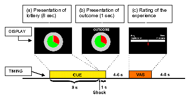Figure 1: Display on subjects' screens and timing of activity during the passive phase of the experiment

2 Experimental design and procedures

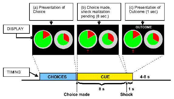Figure 2: Display on subjects' screens and timing of activity during the active phase of the experiment

A total of 37 subjects participated in the study. Seventeen were male and 20 were female. The average age of participants was 25 years, and 17 of the 37 subjects were students. Each individual participated in the experiment at a separate time, and thus during each session only one participant was present. Sessions were conducted at the Emory University Hospital in Atlanta, Georgia, USA. Each session lasted an average of two hours and each participant was awarded $40 at the end of his session. Each session consisted of a series of 180 trials, in which in each trial subjects had the possibility of receiving an electric shock. Shocks were delivered using a Grass SD-9 stimulator⁶ through shielded, gold electrodes placed 2-4 cm apart on the dorsum of the left foot. Each shock was a monophasic pulse of 10-20 ms duration. During their session, individuals were lying down in an MRI scanner.⁷ While in the scanner, the participant observed a computer screen and used a handheld device to submit their decisions.

At the beginning of the session, the voltage range was titrated for each participant. The detection threshold was determined by delivering pulses starting at zero volts and increasing the voltage until the individual indicated that he could feel them. The voltage was increased further, while each participant was instructed, "When you feel that you absolutely cannot bear any stronger shock, let us know - this will be set as your maximum; we will not use this value for the experiment, but rather to establish a scale. You will never receive a shock of maximum value." The purpose of this procedure was to control for the heterogeneity of the skin resistance between subjects and to administer a range of potentially painful and salient stimuli in an ethical manner. We measured the strength of the shock administered to an individual by the parameter s, where the associated voltage for an individual was V = s(V_min-V_min) + V_min, where V_min is the detection threshold (not painful, but just noticeable) and V_max is the maximum value for the individual. For the remainder of the experiment, s took on values of 0.1, 0.3, 0.6, and 0.9.

After the voltage titration, the first phase of the experiment, which we call the passive phase, began. The software package, COGENT 2000 (FIL, University College London), was used for stimulus presentation and response acquisition. The passive phase consisted of 120 trials. The sequence of activity in each trial is illustrated in Figure 1. The upper part of the figure illustrates the displays that subjects observed on their computer screen. The lower part of the figure shows the timing of events within each trial. At the beginning of each trial, each participant was presented with a pie chart, called the cue, which conveyed both the magnitude of the potential impending shock and the probability with which it would be received. The magnitude of the shock was indicated by the size of an inner circle relative to an outer gray circle. This outer circle corresponded to the individual's maximum tolerable voltage, V_max. The area of the inner circle was V_s, where s equaled 0.1, 0.3, 0.6, or 0.9, depending on the trial. The probability was indicated by the proportion of the inner circle colored in red on participants' computer screens, which is shown in Figure 1 as the percentage of the inner circle shaded in the darker color. The five possible probabilities were 1/6, 1/3, 2/3, 5/6, and 1. The particular example shown on the left part of Figure 1 depicts a voltage level with the value of s = 0.6, and a 1/3 probability of the shock being applied. The four possible voltage levels and five possible probabilities yielded 20 voltage-probability combinations, each of which was presented 6 times in the 120 trials that constituted the passive phase of the experiment.

After the cue was presented for 8 seconds, the shock was then delivered with the appropriate probability.⁸ The word, "outcome," as shown in the second image located in the upper middle of Figure 1, was presented concurrently with the delivery of the shock on those trials in which a shock occurred. It also appeared at the same point in time on those trials in which a shock was not delivered, providing an indicator to the participant that the trial was over. It remained on display for one second⁹, after which a display consisting of a visual analog scale appeared on the participant's screen. The display is shown in the upper-right part of Figure 1. The subject was then required to rate the experience of the trial in a range between "very unpleasant" and "very pleasant." To indicate his rating, he marked a location on the scale, using a cursor operated by hand. The process then continued to the next trial.

The next phase of the session, which we call the Active Phase, consisted of 60 trials. In each trial, individuals were required to choose between two of the probability/shock combinations that were presented in the passive phase. The available choices differed from one trial to the next. Figure 2 shows an example of the displays that appeared on participants' screens during a typical trial as well as the timing of a trial. At the beginning of each round, a display similar to the one shown in the upper left of the figure appeared. The figure shows two lotteries presented side by side, and subjects were required to choose one of the two using the keypad provided to them. The two options available in a given trial always had the property that one alternative specified both a higher voltage shock as well as lower probability than the other alternative. For instance, the example shown in Figure 2 represents a choice between 1/6 chance of a shock with s = 0.9 vs. a 1/3 chance of a shock with s = 0.6. The larger inner circle represents the larger shock (i.e., s = 0.9); the probability is represented by the proportion of the area of the inner circle that is colored in red.

After the participant made his choice, there was an 8 second interval, in which the display was augmented by an arrow indicating the lottery chosen. After the 8 seconds had elapsed, the outcome was realized and the word "outcome" was included on the display for 1 second, as shown in the upper right part of Figure 2. Then, the current trial ended and the next of the 60 trials that made up the active phase began. The experimental session ended after the active phase was completed.

3 Results

The results show that the data are consistent with probability weighting, and that the sample parameter value of the particular probability weighting function we estimate is very close to the values reported in previous studies. We first tested the hypothesis that expected utility theory can explain our data. To do so, we estimated the value of a prospect or lottery, V(L)=sum_ipi(p_i)U(x_i), where p_i is the probability of outcome x_i. using the specification for probability weighting of Tversky and Kahneman (1992).¹⁰ Under this specification, the value of a prospect that yields non-positive payoffs under all possible realizations is given by:

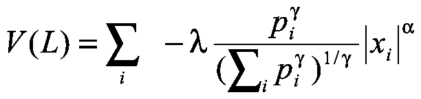(1)

The expected utility hypothesis is consistent only with gamma = 1. In contrast, previous estimates of the median value of gamma for samples of experimental participants incurring hypothetical monetary losses are .69 obtained by Tversky and Kahneman (1992) and .70 observed by Abdellaoui (2000). All values gamma in (0,1) imply an inverted S-shape probability weighting function, in which relatively low probabilities are over weighted, and relatively high probabilities are underweighted (probabilities of 0 and 1 receive accurate weight for all gamma in (0,1].) The parameter lambda is a scaling factor. The parameter alpha measures the convexity (or concavity) of the utility function. The variable x_i is the voltage of the shocks administered. There is no guide from prior research about the appropriate level of lambda or alpha because there is no reason to believe that the scale or curvature of the utility function would be the same for electric shocks as for the real and hypothetical monetary payments previous authors have investigated, though there is evidence (Stevens, 1961) that the psychological reaction to the intensity of electric shocks applied to the fingers follows a power function with an exponent of approximately 3.5.

Because we did not elicit certainty equivalents in our experiments, we used a ranking procedure to derive a measure of the relative value of each of the 20 lotteries to each subject. There were 190 possible lottery pairs, but we only observed actual choices for 60 pairs for each individual (i.e., all those pairs for which there was a tradeoff between higher probability and higher pain determined by the value of s). For these sixty pairs, individuals' choices yielded a revealed preference between the two lotteries. To construct "revealed" preferences for the other 130 pairs (those that were not presented to the subject), we applied a strict dominance criterion. We assumed that individual i would have always chosen a lottery with a lower probability and lower pain over a higher pain, higher probability option.¹¹ We determined the rank or "relative preference" of each of the 20 lotteries based on the percentage of times that it was "revealed preferred" to other lotteries. This procedure yields a complete and transitive preference ordering of the 20 lotteries. We then used the ranked lotteries, determined separately for each individual participant, as data to fit the specification in (1). The parameters, alpha, lambda, and gamma, were estimated jointly using nonlinear least squares regression with normally distributed errors.¹²

The mean estimated value of the probability weighting parameter gamma for the 37 subjects was 0.659, with a standard deviation among the 37 individual estimates of 0.218. The median estimated value was 0.685.¹³ Females tended to have higher estimates (median=0.769 vs. 0.570 for males), but the difference between the two genders was not significant. We then classified our subjects into groups based on whether (a) the EUT value of 1 or (b) the value of gamma estimated in Tversky and Kahneman (1992) of 0.69, fell within the 95% confidence interval of the estimated individual gamma (individual estimated values and standard errors can be found in the Appendix). Forty-six percent (17 out of 37) of our subjects' estimated probability weighting parameters were consistent with Tversky-Kahneman but not with EUT, whereas 14% (5 out of 37) were consistent with EUT but not with Tversky-Kahneman. The rest of the subjects were consistent with both values (24%) or with neither (16%).¹⁴ Figure 3 shows the proportion of estimated values that fell into the four categories listed above.

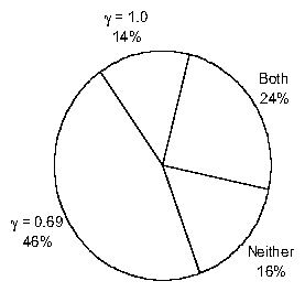Figure 3: Percentage of subjects for whom the gamma values of 1 or 0.69 fell within the 95% confidence interval of their individual gamma estimate

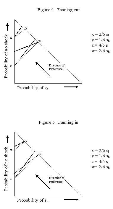We now consider the incidence of common ratio violations in the data. Let s_h be the more painful and s_l be the less painful of two alternative potential shocks presented as a pair-wise choice, and let p_h and p_l be the higher and lower probabilities among the two alternatives, respectively. In our experiment, common ratio violations were observed when the lottery (s_h, p_l = 1/6) was chosen over (s_l, p_h = 2/6), but (s_l, p_h = 4/6) was chosen over (s_h, p_l = 2/6), or alternatively, vice versa. Within the context of the Marschak-Machina triangle and under the assumption that the indifference curves are linear¹⁵, the first sequence of decisions corresponds to "fanning in" of indifference curves; the second sequence, on the other hand, is consistent with "fanning out" of indifference curves. Figure 4 depicts the Marschak-Machina (M-M) triangle with indifference lines. An individual who is indifferent between x and y, and indifferent between z and w will have parallel indifference lines passing through each of the two pairs of points. However, if the individual prefers x to y, then her indifference line will have a higher slope as shown by the darker dashed line passing through x in the figure. Under EUT, if x is preferred to y, then z is preferred to w (shown by the lighter dashed line passing through z). A choice of w would constitute a common ratio violation, and would imply that the indifference line passing through w has a smaller slope than the one passing through x, as depicted by the darker solid line in the figure. Note that the choice of x and w means that the indifference curves are "fanning out". Similarly, Figure 5 depicts "fanning in." In the active phase of the experiment, there were a total of six instances in which common ratio violations could occur. The observed type and number of violations per subject can be found in the Appendix.

The results show that the average number of common ratio violations by individual was 1.95 with a standard deviation of 1.39, which is clearly different from the prediction of EUT.¹⁶ There is a tendency to commit more fanning out violations than fanning in violations. This is not surprising, as indifference curves that fan out are consistent with overweighting of small probabilities. About 68% of the subjects (25 out of 37) committed one or more fanning out violations, whereas about 46% (17 out of 37) committed one or more fanning in violations. The Fisher exact test shows that the null hypothesis that the proportion of subjects who commit at least one fanning in and fanning out violations are the same is rejected in favor of the alternative of more people committing fanning out violations (p = 0.049; one-tailed). Five subjects committed fanning in violations only; in contrast, seventeen subjects committed uniquely fanning out violations. Finally, there were small differences between the average number of violations committed by females (2.10; std = 1.37) as compared to males (1.76, std = 1.43).

We also considered whether there was consistency between our above classification of subjects (Figure 3) and the observed number of common ratio violations. None of the five subjects whose estimated gamma value was consistent with only EUT committed more than two common ratio violations. In contrast, the number of violations by subjects with estimated gamma significantly less than 1 ranged from zero to five. Overall, however, there are no statistically significant differences in the median number of violations between these two groups (p > 0.188, one-tailed).

Although the overall fanning effect was as predicted, there were large individual differences. Some participants showed no fanning; whereas others showed fanning in the opposite directions. Were these consistent differences, or just random variation? We found that, within an individual, the direction of violations was consistent, in a specific sense, with their overall choice behavior in the 60 trials of the active phase. To study this consistency, we computed a "mean fanning effect" for each subject from the six instances where individuals could switch preferences, and we asked whether this effect could be predicted from an index of fanning computed from the remaining 54 cases. Fanning out is indicated by a lower tendency to choose the low-probability-high-shock option when overall shock probabilities are smaller (i.e., closer to the top of the M-M triangle in Figure 4). Using the 54 decisions between which common ratio violations cannot be detected from decisions, we conducted a regression with the chosen lottery as the dependent variable. The independent variables were the difference in the logs of the shock intensity of the two options, the difference in the logs of the probabilities of a shock under the two options, and the sum of the two probabilities of receiving a shock under the two options. The regression coefficient for this last variable, which is a measure of the distance from the top of the M-M triangle, was our index of the fanning effect. The coefficient takes on a smaller value, the more the tendency toward fanning out. We found a positive correlation between the individual estimated coefficients of the fanning index, and whether they committed more fanning out than fanning in violations (r=.31, t(35)=1.95, p=.0293, one-tailed).¹⁷ Thus, individuals differ in a consistent manner in the direction and magnitude of this effect.

4 Discussion

In this paper we provide evidence that non-linear probability weighting, which has been observed when prospective losses are framed in terms of money, also occur in lottery choices when real adverse outcomes are induced with a non-monetary medium. As in previous studies, our estimated values of the probability weighting parameters provide little support for EUT. We find that about 14% of our subjects' estimated probability weighting parameters is consistent with EUT. In contrast, about 46% of the subjects overweight small probabilities and underweight large probabilities, exhibiting a typical inverted S-shape probability weighting function. Furthermore, the estimated sample median probability weighting parameter we obtain is closely in line with values reported in previous studies. This suggests that probability weighting acts in a similar manner for lottery choice when outcomes are measured in terms of physical pain as well as for hypothetical monetary transfers. This result is consistent with the conjecture that probability weighting is a general phenomenon, and independent of the source of disutility.

We also find that common ratio violations, which are inconsistent with EUT, are widespread. A greater proportion of subjects commit violations consistent with indifference curves that fan out than with fanning in. However, there are large individual differences in the direction and incidence of the violations. Despite these differences, we were able to determine that the direction of subjects' violations is largely consistent with their overall choice behavior, and not random.

In our view, the results we obtain are encouraging evidence that traditional methodologies used in economics and psychology to study decisions in the domain of negative payoffs lead to the same principles of decision making as those applied in decisions over non-monetary media with real losses. Indeed, we reach almost identical conclusions to previous studies. Our results also suggest a conjecture that in the domain of positive payoffs, the probability weighting parameters estimated for monetary payments would carry over to non-monetary media. In the future, we believe that the methodology of applying physical pain to study decision making may be used to explore the robustness of other behavioral anomalies observed in the laboratory that occur when payoffs are negative.

References

Abdellaoui, M. (2000). Parameter-free elicitation of the probability weighting function. Management Science, 46, 1497-1512.

Allais, M. (1953). Le comportement de l'homme rationnel devant le risque: Critique des postulats et axioms de l'école américaine. Econometrica, 21, 503-546.

Ariely, D., Loewenstein, G., & Prelec, D. (2003). Coherent arbitrariness: Stable demand curves without stable preferences, Quarterly Journal of Economics, 118, 73-105.

Baltussen, G., Post, T., Van den Assem, M. J., & Thaler, R. (2007). Reference-dependent risk attitudes: Evidence from versions of Deal or No Deal with different stakes. Tinbergen Institute/Erasmus University working paper.

Berns, G., Capra, M., Chappelow, J., Moore, S., & Noussair, C. (2006). Neurobiological probability weighting functions over losses. Emory University working paper.

Bleichrodt, H. & Pinto, J. (2000). A Parameter-free elicitation of the probability weighting function in medical decision analysis. Management Science, 46, 1485-1496.

Camerer, C. & Ho, T.-H. (1994). Violations of betweenness axiom and nonlinearity in probability. Journal of Risk and Uncertainty, 8, 167-196.

Coursey, D. L., Hovis, J. L., & Schulze, W. D. (1987). The disparity between willingness to accept and willingness to pay measures of value. Quarterly Journal of Economics, 102, 678-690.

De Roos, N., & Sarafidis, Y. (2006). Decision making under risk in Deal or No Deal. University of Sydney and CRA International working paper.

Gonzalez, R. and G. Wu (1999). On the Shape of the Probability Weighting Function, Cognitive Psychology, 38, 129-166.

Harless D. & Camerer, C. (1994). The Predictive Utility of Generalized Expected Utility Theories. Econometrica, 62, 1251-1289.

Hey, J. & Orme, C. (1994). Investigating Generalizations of Expected Utility Theory Using Experimental Data. Econometrica, 62, 1291-1326.

Holt, C. & Laury, S. (2005). Further reflections on prospect theory., Georgia State University working paper.

Kahneman, D., & Tversky, A. (1979). Prospect theory: An analysis of decision under risk. Econometrica, 47, 263-291.

Loomes, G. (1991). Evidence of a new violation of the independence axiom. Journal of Risk and Uncertainty, 4, 91-108.

Malinvaud, E. (1952). Note on von-Neumann-Morgenstern's strong independence axiom. Econometrica, 20, 679. Machina, M. (1982). Expected Utility Analysis without the Independence Axiom. Econometrica, 50, 277-323.

Mason, C., Shogren, J., Settle, C., & List, J. (2005). Investigating risky choices over losses using experimental data. Journal of Risk and Uncertainty, 31, 187-215.

Prelec, D. (1998). The probability weighting function. Econometrica, 66, 497-527.

Quiggin, J. (1993). Generalized expected utility theory: The rank dependent model. Heidelberg, Germany: Springer Verlag Publishers.

Smith, V. (1982). Microeconomic systems as an experimental science. American Economic Review, 72, 923-955.

Starmer, C., (2000). Developments in non-expected utility theory: The Hunt for a descriptive theory of choice under risk. Journal of Economic Literature, 38, 332-382.

Starmer C. & Sugden, R. (1989). Violations of the independence axiom in common ratio problems: An experimental test of some competing hypotheses. Annals of Operations Research, 19, 79-102.

Tversky, A. & Fox, C. (1995). Weighing risk and uncertainty. Psychological Review, 102, 269-323.

Tversky, A., & Kahneman, D. (1992). Advances in prospect theory: cumulative representations of uncertainty. Journal of Risk and Uncertainty, 5, 297-323.

Wakker, P. & Deneffe, D. (1996). Eliciting von Neumann-Morgenstern utilities when probabilities are distorted or unknown. Management Science, 42, 1676-1690.

Wu G. & Gonzalez, R. (1996). Curvature of the probability weighting function, Management Science. 42, 1676-1690.

Appendix.

Estimates of individual gamma parameters, and type and number of fanning violations

Subject	Sex	Est. gamma	Std. err.	Fan out	Fan in
1	F	1.0127890	0.0796662	2	0
2	F	0.3915420	0.1450381	0	0
3	M	0.5452798	0.1469481	1	0
4	F	0.8426407	0.0907564	3	0
5	F	0.7069833	0.1078082	2	0
6	M	0.7641525	0.1032662	1	2
7	M	0.5423165	0.1307505	1	0
8	M	0.9610685	0.0648182	1	0
9	F	0.4574296	0.1382386	1	0
10	M	0.4818398	0.1515036	0	1
11	M	0.8285788	0.1330844	1	1
12	F	0.2973379	0.1289225	0	0
13	M	0.3323089	0.1426116	0	0
14	M	0.6006711	0.1175138	0	0
15	F	0.2707158	0.1300445	1	0
16	F	0.4599991	0.0932652	1	2
17	M	0.6856989	0.1550794	0	5
18	F	0.7670457	0.1119126	3	1
19	F	0.7078283	0.1031506	4	0
20	M	0.4624952	0.1245585	0	0
21	F	1.0176710	0.0874302	1	0
22	M	0.8409525	0.0796012	1	1
23	M	0.5703915	0.1138435	0	1
24	F	0.9963527	0.1260562	2	0
25	M	0.6664429	0.1116457	1	2
26	F	0.4039314	0.1187758	0	0
27	F	1.0344640	0.0756161	0	1
28	F	0.7988346	0.1216859	1	1
29	M	0.5665003	0.1288915	2	0
30	F	0.7718875	0.1614382	0	4
31	M	0.5567840	0.1339346	2	2
32	M	0.3608489	0.1084658	0	1
33	F	0.7960892	0.1137703	2	2
34	F	0.9279254	0.1309254	3	0
35	M	0.7009950	0.1272274	2	1
36	F	0.7771528	0.0873558	1	2
37	F	0.4700133	0.1200721	2	0

Footnotes:

¹Corresponding author, Department of Economics, Emory University, 1602 Fishburne Drive, Atlanta, GA 30322. Email: mcapra@emory.edu. Supported by grants from the National Institute on Drug Abuse (DA016434 and DA20116). We would like to thank an anonymous referee and the editor of this journal, Jonathan Baron, for working out the intricacies of individual differences and other invaluable suggestions. All errors are ours.

²Common ratio violations also result when the independence axiom on preferences is relaxed or violated. See Malinvaud (1952) for a discussion of the relationship between the independence axiom and expected utility theory. See Machina (1982) for an analysis of the implications of relaxing the assumption that the independence axiom holds.

³Some recent studies using real decisions of participants in the TV game show "Deal or No Deal" also find support for generalized expected utility models when decisions are over possible large sums of money. De Roos and Sarafidis (2006) find that rank dependent utility models are better at describing decisions. Using cross-country data from the same game, Baltusen et al. (2007) find that theories that include reference dependence, an assumption of Prospect Theory, but not EUT, are better at describing observed decisions.

⁴ Bleichrodt and Pinto (2000) also study choices under risk over non-monetary losses, but their outcomes are hypothetical medical maladies.

⁵ Indeed, self-reports of participants, who evaluated the experience after the shocks, show that shocks were perceived negatively and shocks of different voltages were preceived differently from each other. As described in the procedures, participants were required to rate the experience of each trial of the experiment on a scale, which ranged from "very unpleasant" to "very pleasant". We find that the stronger the shock was, the more unpleasant the experience was.

⁶ The Grass stimulator (West Warwick, RI) was modified by attaching a servo-controlled motor to the voltage potentiometer. The motor allowed for computer control of the voltage level without comprising the safety of the electrical isolation in the stimulator. The motor was controlled by a laptop through a serial interface.

⁷ Skin conductance responses to the shocks were also registered. The analysis of the fMRI and the skin conductance response data are reported in a companion paper (see Berns et al, 2006).

⁸ The outcomes were predetermined (although unknown beforehand to participants) to ensure that there would be at least one trial under each of the 20 conditions (4 different voltages times 5 different probabilities) in each of the three 60-trial fMRI scan runs. Although the outcomes were predetermined, the total number of shocks received in each of the conditions reflected the actual probabilities.

⁹Following the shock, the cue remained visible for another 1 second to prevent conditioning to the cue offset.

¹⁰ Our parametric estimations of the probability weighting function using alternative functional forms such as those proposed in Tversky and Fox (1995), and Wu and Gonzalez (1996) result in similar conclusion.

¹¹ Implicit is the assumption that in decisions in which there are no tradeoffs between probability and pain (where one alternative has both higher voltage and probability than the other), the subject would not make common ratio violations.

¹²Other authors such as Tversky and Kahneman, (1992), Camerer and Ho (1994) and Tversky and Fox (1995) have also made parametric estimates of the probability weighting function and the utility function. Some authors such as Abdellaoui (2000) and Bleichrodt and Pinto (2000), have used parameter free estimations employing a trade-off technique of Wakker and Deneffe (1996). Overall, however, there seems to be little difference in the median values of the estimated gamma parameters using either method.

¹³The estimated parameters were robust to a wide range of economically relevant initial values.

¹⁴ Using the trade-off technique, Bleichrodt and Pinto (2000) found that over 80% of their subjects exhibited a probability weighting function with lower and upper subadditivity (i.e, the inverted S-shape). Other authors do not report individual data for their entire sample. In line with Bleichrodt and Pinto's results, we find that about 84% of or subjects exhibit probability weighting consistent with subadditivity.

¹⁵We are aware that with only two points in the border of the MM triangle, we cannot make inferences about the shapes of the indifference curves. We use linear indifference curves in the figures for the specific purpose of illustrating the fanning effects in an easy manner.

¹⁶ The Friedman test for no differences between the observe number of violations versus the number that would happen randomly can be rejected (Chi-square 10.80; df = 1; p < 0.01).

¹⁷With respect to the six critical cases where preference reversals can be observed, a reliability test also shows that decisions are consistent (Cronbach's alpha = 0.45).

File translated from T_EX by T_TH, version 3.74.
On 25 Aug 2007, 11:52.