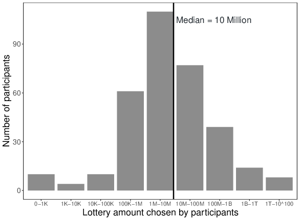
| Figure 1: Frequency distribution of participants’ preferred lottery win (K = thousand, M = million, B = billion, T = trillion) for Study 1. |
Judgment and Decision Making, Vol. 17, No. 6, November 2022, pp. 1229-1254
Do people believe that you can have too much money? The relationship between hypothetical lottery wins and expected happinessTessa Haesevoets* Kim Dierckx# Alain Van Hiel$ |
Abstract: Do people think that there is such a thing as too much money? The present research investigated this question in the context of hypothetical lottery wins. By employing a mental simulation approach, we were able to examine how people respond to increasing envisioned jackpot amounts, and whether there are individual differences in people’s reactions. Across five empirical studies (total N = 1,504), we consistently found that, overall, the relationship between imagined lottery wins and expected happiness is characterized by an inverted U-shaped curve, with expected happiness being highest around an envisioned win of roughly 10 million pounds. Both lower and higher envisioned wins reduced participants’ overall expected happiness. In addition to this overall pattern, we identified three clusters of participants who react differently to expected increases in wealth. These clusters mainly differed in terms of how soon the top of the expected happiness curve was reached, and if and when the curve started to drop. Finally, we also found some interesting cluster differences in terms of participants’ prosocial and proself motivations.
Keywords: hypothetical lottery wins; expected happiness; inverted U-curve; cluster analysis; individual differences
“You can never be too rich or too thin” – attributed to Wallis Simpson
The link between money and happiness has been a central topic of scientific study, with most prior studies either investigating how people’s income level correlates with their actual happiness rating or comparing the actual happiness level of wealthy people (millionaires and/or lottery winners) with that of a control group from the general population. Although many of these studies have reported a positive connection between wealth and happiness (e.g., Lindqvist et al., 2020; Oswald & Winkelmann, 2019; Stevenson & Wolfers, 2013), there is also some evidence that wealthy people are not necessarily much happier — and sometimes even less happy — than those who are less wealthy (e.g., Brickman et al., 1978; Nissle & Bschor, 2002; Lutter, 2007; Raschke, 2019). The present study aims to provide a fresh look at this classical topic, and this by examining if people indeed believe that money will buy them happiness and whether they think it is possible to have too much money. To this end, instead of investigating the “true” relationship between money and happiness (as has been done in most prior studies in this domain), we explored people’s naïve theories of the money-happiness relation in the context of hypothetical lottery wins. The objectives of our study were threefold.
The first objective of our research was to examine the exact nature of the relationship between hypothetical lottery wins and expected happiness. Specifically, we employed a mental simulation approach to investigate how various imagined jackpot amounts influence one’s expected happiness level. This approach allowed us to ask whether, generally speaking, people’s expected happiness continues to rise when the amount of money that they imagine winning increases, or whether there is a certain inflection point after which higher envisioned wins no longer increase — and possible even reduce — expected happiness. In testing which of these perspectives most accurately reflects people’s general preference pattern, we also aimed to identify what people ‘overall’ consider to be the optimal lottery amount that they believe will bring them the most happiness.
It is plausible that people do not react all alike to expected increases in wealth. Therefore, as a second research objective, we investigated whether the shape of the relationship between hypothetical lottery wins and expected happiness varies across individuals. More specifically, we asked whether we could identify different clusters of people who react differently to increasing envisioned jackpot amounts. Which clusters then might exist? We expected a first cluster of people who react according to the non-satiation (or, as it is more commonly called, the ‘more-is-better’) assumption (Smith, 1976). This assumption holds that more of a certain good is better than less of it. As such, it can be predicted that for some people expected happiness will rise indefinitely with the amount of money that one supposedly won (resulting in a boundlessly rising curve). Seligman and Csikszentmihalyi (2014) have, however, noted that “what makes people happy in small doses does not necessarily add satisfaction in larger amounts” (p. 11). The principle of diminishing returns speaks to this issue (Brue, 1993). If this principle holds, then a second cluster of people might emerge, showing an initial increase in expected happiness when the amount of money that one allegedly won increases, but for whom expected happiness stagnates at large envisioned wins (resulting in diminishing return curve). Finally, prior research has shown that ordinarily beneficial antecedents can become counterproductive when taken too far, a phenomenon which is known as the ‘too-much-of-a-good-thing’ effect (Grant & Schwartz, 2011). As such, we anticipate a third cluster of people who react with decreased happiness when the imagined lottery wins cross a specific threshold (resulting in an inverted U-curve).
The third and final objective of our research was to explore the nature of potential cluster differences. One concept that may be particularly relevant in this context is Social Value Orientation (SVO), which refers to stable individual differences in preferences for particular distributions of outcomes for oneself and others (Messick & McClintock, 1968; Van Lange, 1999). The literature typically distinguishes individuals with a prosocial orientation (who tend to maximize outcomes for self and others, and minimize differences between these outcomes) and those with a proself orientation (who tend to maximize outcomes for themselves, either in an absolute or a relative sense; see Kuhlman & Marshello, 1975; McClintock & Liebrand, 1988; Van Lange & Kuhlman, 1994). We expect the cluster in which no satiation effect is present (and who thus reacts according to the ‘more-is-better’ assumption) to be more proself and less prosocially oriented than the other two clusters for whom happiness is expected to stagnate or decrease at large envisioned wins. Importantly, however, people might display the hypothesized preference patterns for different reasons. Therefore, besides pitting the general prosocial and proself dimension against each other (as is done in most measures of SVO), we additionally examined whether and how the hypothesized clusters differ from each other in terms of more specific prosocial and proself motivational traits. As specific prosocial motives, we included fairness, altruism, and concern for others. As specific proself motives, we included greed, competitiveness, and entitlement.
To test the aforementioned research objectives, we conducted five empirical studies (see Table 1 for an overview). Given that our research focusses on the relationship between hypothetical lottery wins and expected happiness (rather than the association between real money and actual happiness), we relied on a mental simulation manipulation (see Sharif et al., 2021, for a recent application of this methodology) that required participants to vividly imagine winning particular jackpot amounts in a lottery. The aim of our first study was to obtain a general estimate of which particular lottery prize participants would prefer to win in a lottery. Using various different research designs, our four subsequent studies all employed an experimental approach to map how different jackpot amounts affect participants’ expected happiness (Objective 1). Our last three studies additionally also explored the existence of individual difference patterns in participants’ preferences for different jackpot amounts (Objective 2), as well as the defining motivations underlying these individual difference patterns (Objective 3). Unless mentioned otherwise, the data were analyzed using SPSS (version 28.0.0). The data, data analysis scripts, codebooks, and Supplementary Material (Online Appendix) can be accessed through https://osf.io/j9sxa.
Table 1: Overview of the five empirical studies (total N = 1,504).
Study N Presentation order Test of objective(s) Study 1 333 - Objective 1 Study 2 275 - Objective 1 Study 3 220 Fixed Objectives 1, 2, & 3 Study 4 327 Random Objectives 1, 2, & 3 Study 5 349 Random Objectives 1, 2, & 3
We recruited a sample of 333 adult UK participants through Prolific (125 men, Mage = 34.17, SD = 13.11; more descriptive statistics can be found in Appendix A). At the start of the study, participants were presented with the following introductory statement:
Please try to imagine that there is a new worldwide lottery game, which is similar to Euro Millions. With this new lottery game, you can win an infinitely large amount of money (that is, this new lottery game has no upper boundary, except for “all the money in the world”).
After reading this statement, participants were asked to mentally simulate this situation and subsequently answer the following open-ended question: “Which amount (in GBP) would you prefer to win with this new lottery game?” Participants could answer this question by entering their preferred amount.
The amounts chosen by participants ranged from zero up to a googol (i.e., the digit 1 followed by 100 zeros), with the median amount chosen by participants being 10 million pounds. A closer look at Figure 1, however, illustrates that the majority of the participants (more than 75%) chose an amount between 100 thousand pounds and 100 million pounds. As such, these results provide a first indication that, for most participants, there indeed seems to be an upper limit to their desire for money. Moreover, these findings also indicate that the preferred lottery win varies considerably across participants (with some preferring rather small and others preferring really large wins).
Figure 1: Frequency distribution of participants’ preferred lottery win (K = thousand, M = million, B = billion, T = trillion) for Study 1.
In our second study, we used an experimental approach to statistically test which lottery amount participants expect will bring them most happiness. To this end, we recruited a sample of 296 participants who lived in the UK through Prolific. Twenty-one participants (7.1%) were excluded from the analyses because they failed our manipulation check (see below). The remaining 275 participants (106 men) were on average 35.76 years old (SD = 12.90). More descriptive statistics of the sample (education and income) can be found in Appendix A.
At the beginning of the study, participants were presented with the same introductory statement as in Study 1. After reading this statement, participants were randomly assigned to one of the five experimental conditions that varied the allegedly won amount of money. In this vein, we included the median amount of Study 1 (i.e., 10 million pounds) as well as two smaller amounts and two larger amounts. Specifically, participants were asked to mentally simulate that they had won 1 thousand pounds in the first condition (n = 60; 21.8%), 1 million pounds in the second condition (n = 46; 16.7%), 10 million pounds in the third condition (n = 52; 18.9%), 10 billion pounds in the fourth condition (n = 61; 22.2%), and 10 trillion pounds in the fifth condition (n = 56; 20.4%).These lottery amounts were presented to participants both in numbers (e.g., 1,000) and in words (e.g., one thousand).
We first asked participants, as a manipulation check, how much money they supposedly won, and provided the five included lottery amounts as response options. The 21 participants whose response was inconsistent with their allocated condition were removed from the analyses (2 to 6 per condition). In all five conditions, we subsequently asked participants to answer the following questions: “To what extent would you be satisfied with this amount?”, “To what extent would you be happy with this amount?”, and “To what extent would you be pleased with this amount?” Participants could answer these questions on a 11-point Likert scale ranging from (1) not at all to (11) very much so. Because responses on these three items all loaded strongly on a single factor (which explained 92.8% of the variance; all factor loadings > .93), they were averaged into a general expected happiness scale (M = 9.44, SD = 2.54, Cronbach’s α = .96).
As shown in Figure 2, the relationship between the hypothetical lottery wins and expected happiness seems to be characterized by an inverted U-shape. To formally substantiate the presence of a “cutoff” or breakpoint in expected happiness, we used Simonsohn’s (2018) two-lines approach. This technique formally tests the existence of an inverted U-shaped relation between variables by simultaneously estimating two regression lines, one for lower values and one for higher values of the predictor. Using the “Robin Hood” algorithm (Simonsohn, 2018), this method automatically derives the optimal breakpoint or cutoff point between the lines. An inverted U-relation is formally present if the slope of the first regression line is significant and positive and the slope of the second regression line is significant and negative. The results of this analysis showed that the slope of the first regression line was significantly positive (b = 1.23, p < .001) whereas the slope of the second regression line significantly negative (b = –0.84, p < .001), thereby clearly supporting the existence of an inverted U-shaped relation. Moreover, these results further corroborated the presence of a breakpoint in expected happiness at an envisaged lottery win of 10 million pounds.
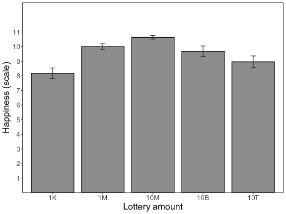
Figure 2: Expected happiness (mean of happy, satisfied, and pleased item) as a function of the different lottery amounts (K = thousand, M = million, T = trillion) for Study 2. Error bars represent standard errors.
The results of Study 2 show that, from a certain point onwards, additional money starts to have an adverse impact on participants’ expected happiness. Study 3 aimed to replicate and extend this finding using a different research methodology. Specifically, we employed a similar setup as in Study 2, but this time we used a within-subjects (instead of a between-subjects) design to administer the different jackpot amounts. An important limitation of manipulating lottery amounts between-subjects in Study 2 is that participants had to judge only one single lottery amount. The use of a within-subjects design in the present study — in which the same participants had to judge multiple lottery amounts — allowed us to not only undertake a more fine-grained investigation of how the different jackpot amounts affect expected happiness but also to test for the possible individual difference patterns.
We recruited 229 UK participants through Prolific. To identify participants who answered with insufficient care, we deployed an attention check (based on Meade & Craig, 2012). Nine participants (3.9%) failed this attention check question, and, as a result, their responses were excluded from further analyses. The remaining 220 participants consisted of 67 males. They were on average 34.14 years old (SD = 13.00; for more descriptive statistics of the sample, see Appendix A).
Participants were presented with the same introductory statement as in the previous two studies. In the present study, we included the following 12 lottery amounts (which were expressed in GBP): 1 thousand, 10 thousand, 100 thousand, 1 million, 10 million, 100 million, 1 billion, 10 billion, 100 billion, 1 trillion, 10 trillion, and “all the money in the world”. For each of these 12 amounts, participants were asked to answer the following question: “To what extent would you be satisfied with this particular amount?” (1 = not at all, 11 = very much so). This item was randomly selected from the three items that were used in Study 2 (given that they all three probed the same underlying construct). The 12 included lottery amounts were presented to participants in a fixed order, starting with the lowest and ending with the highest amount.
At the end of the study, participants’ social value orientation was measured using the six primary items of the SVO Slider Measure of Murphy et al. (2011), which yields a reliable unidimensional index of an individual’s general social preferences. Each of these six items measures participants’ preferences for particular distributions of valuable points between themselves and another person (see Appendix B for details). An important advantage of this measure is that it assesses participants’ social value orientation on a continuous scale in terms of an angle. A positive angle indicates a positive concern for the payoff of the other person (increasing concern for others), while a negative angular value indicates a negative concern for the payoff of the other person (increasing concern for the self). Thus a larger SVO angle indicates a greater prosocial preference (Mangle = 28.87, SD = 13.65).
Figure 3 shows that the relationship between the hypothetical lottery wins and expected happiness seems to be characterized by an inverted U function. We again used Simonsohn’s (2018) two-lines approach to test the existence of an inverted U-shaped relation. The results (using all 12 lottery amounts) clearly support the existence of an inverted U-shape: The slope of the first regression line was significantly positive (b = 1.09, p = .001), whereas the slope of the second regression line was significantly negative (b = –0.51, p = .001). Analogous to Study 2, the breakpoint was again estimated at an envisioned win of 10 million pounds.1
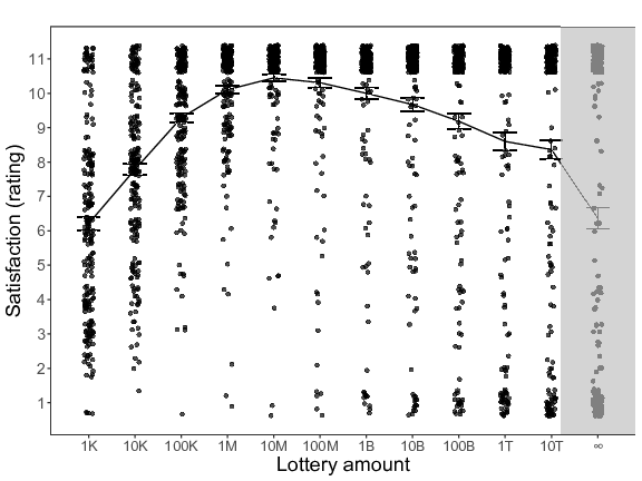
Figure 3: Expected happiness (satisfaction rating) as a function of the different lottery amounts (K = thousand, M = million, B = billion, T = trillion) for Study 3. Error bars represent standard errors.
Importantly, the existence of such a general preference pattern does not preclude the possibility of distinct clusters of individuals reacting differently to increasing expected lottery wins. Indeed, such an inverted U-curve may arise when a sample consists of various subgroups (i.e., clusters), and the resulting general trend may just reflect the mere mean tendency of distinctive patterns. To test this possibility, we ran two cluster analyses using the k-means function in R: One analysis in which all 12 lottery amounts were included (see the left panel of Figure 4) and one analysis in which the “all the money” condition was excluded (see the right panel of Figure 4). Visual inspection of scree plots and calculation of the “gap statistic” (Tibshirani et al., 2001) revealed that in both analyses the best-fitting model was a model with two clusters.
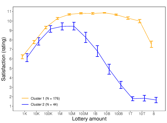
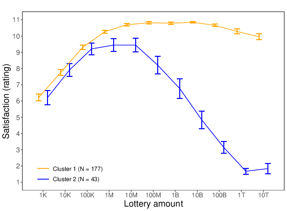
Figure 4: Two different reactions to the increasing lottery amounts (K = thousand, M = million, B = billion, T = trillion) for Study 3. Left panel = with all lottery amounts; right panel = without the “all the money” condition. (Error bars represent standard errors.)
As shown in Figure 4, Cluster 1 consists of a subgroup of participants whose expected satisfaction ratings increased up until an amount of 10 million pounds. From this point onwards, the curve stagnated and this up until 100 billion pounds, after which the curve started to drop. In Cluster 2, participants also initially responded with increased satisfaction to the rising monetary amounts, but here the top of the curve was already reached around 100 thousand pounds. In this second cluster, the curve remained flat between 100 thousand pounds and 10 million pounds. After 10 million pounds, there was a steep downward trend. And, at 1 trillion pounds the expected satisfaction curve even reached almost the lower end of the scale, indicating that participants in this second cluster actually expected to be very dissatisfied with such large envisioned lottery wins. Taking these findings together, it can be concluded that in both analyses the two extracted clusters mainly differed in terms of how soon the top of the satisfaction curve was reached, and from which particular point onwards the curve started to drop — and how deep the curve eventually fell. Interestingly, however, in none of the extracted clusters expected satisfaction increased indefinitely with the envisioned lottery wins.
We subsequently asked whether the two clusters (which were extracted using all 12 lottery amounts; see left panel of Figure 4) differed from each other in terms of participants’ social value orientation. The results of a one-tailed t-test showed that participants’ SVO angle was significantly lower in Cluster 1 (M = 28.08, SD = 13.84) than in Cluster 2 (M = 32.02, SD = 12.50), t(218) = –1.72, p = .044, which indicates (weakly) that participants in Cluster 1 are more proself and less prosocially oriented than those in Cluster 2.
An important drawback of Study 3’s within-subjects design is that it asked participants to rate the different lottery amounts sequentially; that is, one at a time. Based on the evaluability framework (Hsee, 1996; Hsee et al., 1999; Hsee & Zhang, 2010), it can be expected that participants will be much more sensitive to monetary differences when they evaluate multiple jackpot amounts comparatively, rather than sequentially. The results of Study 3 showed that participants in Cluster 1 expected to be equally satisfied with an envisioned win of 10 million pounds as with an envisioned win of 100 billion pounds. It is, however, possible that when these participants have to explicitly choose between 10 million and 100 billion pounds, some of them will prefer to win 10 million pounds whereas others will prefer to win 100 billion pounds. To investigate this interesting possibility, in the present study we employed a pairwise comparison methodology to administer the different lottery wins.
A sample of 327 Belgian participants, recruited through snowball sampling as part of a graduate research project, completed the present study. The sample consisted of 102 males. In terms of age, 16 participants (4.9%) were younger than 20 years, 175 (53.5%) were 21–30 years, 51 (15.6%) were 31-40 years, 21 (6.4%) were 41–50 years, 45 (13.8%) were 51–60 years, and 19 (5.8%) were older than 60 years. More descriptive statistics of the sample (in terms of participants’ education and income level) can be found in Appendix A.
Participants were presented with the same introductory statement as in the previous studies. We included the following 11 lottery amounts: 100 thousand, 500 thousand, 1 million, 5 million, 10 million, 50 million, 100 million, 500 million, 1 billion, 5 billion, and 10 billion. As mentioned above, to administer these amounts we employed a pairwise comparison methodology. The aim of this method is to establish an ordering of objects on a ‘preference’ scale according to specific attributes. Therefore, the paired comparison method splits the ordering process into a series of evaluations carried out on two objects at a time. For each of these pairs, a decision is made which of the two objects is preferred (see Hatzinger & Dittrich, 2012, for more detailed information on this method). In the context of the present study, the objects were embodied by the 11 included lottery amounts — which resulted in a total of 55 pairwise comparisons for each participant to complete. For each of these comparisons, participants were asked the following question: “Which of the following two amounts will bring you most happiness?” The amounts were expressed in EUR (1 EUR equaled approximately 0.90 GBP and 1.10 USD at the time that the present studies were conducted) and the presentation order of the comparisons was randomized. To measure participants’ general social preferences, at the end of the study we again administered the six primary items of the SVO Slider Measure (Mangle = 32.37, SD = 10.77).
A preference scale was constructed to numerically describe participants’ expected happiness of the different lottery amounts. This scale was estimated through a Bradley-Terry probability model using the Prefmod package (Hatzinger & Dittrich, 2012) in R. Bradley-Terry models are a variant of loglinear models (Dittrich et al., 1998; Sinclair, 1982) which assume that, given J objects, the observed number of times in which object j was preferred over object k follows a Poisson distribution. The location of each object on the preference scale is estimated in a worth parameter π j that can be estimated through the following function:
| p(j>k|πj, πk) = |
|
Figure 5 shows that the estimated worth parameters suggest the existence of an inverted U-shaped relation. We again used Simonsohn’s (2018) two-lines approach to formally test the existence of an inverted U-shaped relation. The slope of the first regression line was positive albeit not statistically significant (b = 0.01, p = 220), whereas the slope of the second regression line was significantly negative (b = –0.02, p < 001). Given that the resulting two slopes had opposite signs, but that only one was found to be significant, the null hypothesis that there was no inverted U-shaped relation could not formally be rejected. Interestingly, however, analogous to Studies 2 and 3, the breakpoint was again estimated at an envisaged lottery win of 10 million.
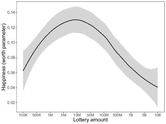
Figure 5: Expected happiness (worth parameter) as a function of the different lottery amounts (K = thousand, M = million, B = billion) for Study 4. The line represents a loess-curve fitted to the estimated worth parameters for visualization purposes.
Individual differences were investigated using the klaR package (Weihs et al., 2005) in R, which allows for the clustering of categorical data by using the k-modes algorithm (Huang, 1997) an extension of the k-means algorithm by MacQueen (1967). Our analysis showed that the best-fitting model contained three clusters (see Figure 6). In Cluster 1, expected happiness continued to rise when the amount of money that one supposedly won increased. In fact, in this first cluster the curve reached its highest point at the largest included jackpot amount of 10 billion euro. The curve of Cluster 2 was characterized by an inverted U-shape (or, more precisely, an inverted V-shape). In this second cluster the peak of the curve was reached at 50 million euro, after which the curve dropped sharply. Finally, in Cluster 3 the curve started quite high and the top of the curve was already reached at 1 million euro. After this point, there was a sharp drop in expected happiness.
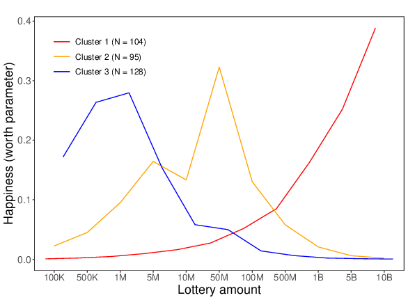
Figure 6: Three different reactions to the increasing lottery amounts (K = thousand, M = million, B = billion) for Study 4. The lines represent the estimated worth parameters of the three clusters.
One-tailed t-tests showed that participants’ SVO angle was significantly lower in Cluster 1 (M = 29.37, SD = 11.83) than in Cluster 2 (M = 33.39, SD = 10.00; t(197) = –2.58, p = .005) and Cluster 3 (M = 34.06, SD = 9.94; t(230) = –3.28, p < .001); with the difference between Cluster 2 and Cluster 3 being non-significant (t(221) = 0.50, p = .310). In line with our predictions, these findings illustrate that participants in Cluster 1 are indeed more proself and less prosocially oriented than those in Clusters 2 and 3.
If we compare the two-cluster solution that we obtained in Study 3 (see Figure 4) with the three-cluster solution that we obtained in Study 4 (see Figure 6), we can see that there are some similarities but also some differences. One notable difference is that in Study 3 the expected satisfaction curve for Cluster 1 flattened out once the optimum was reached, whereas in Study 4 this was not the case in any of the three clusters (i.e., in the first cluster expected happiness continued to rise with increasing money; whereas in the second and third cluster the expected happiness curve immediately dropped after the apex was reached). However, such differences can possibly be ascribed to the use of two different measurement methods (i.e., a within-subjects design in Study 3 and a pairwise forced-comparisons methodology in Study 4). Yet, because these two studies were conducted among two different samples, we are unable to directly compare the two clusters of Study 3 with the three clusters of Study 4. In order to allow for such a direct cluster comparison, in Study 5 we used a setup in which the same participants were presented with both methodologies. That is, in Study 5 all participants were asked to rate the lottery amounts both separately as well as in pairs.
We recruited 370 participants from the UK through Prolific. We employed the same attention check as in Study 3, which led to the exclusion of 21 participants (5.7%). The remaining 349 participants consisted of 131 males. They were on average 34.53 years old (SD = 13.04; see Appendix A for more descriptive statistics of the sample).
The present study consisted of two different measurement moments.
During the first measurement moment, participants were presented with the same introductory statement as in the previous studies. In order to cover the full range of potential wins, we included the following 12 lottery amounts: “no money at all”, 1 thousand, 10 thousand, 100 thousand, 1 million, 10 million, 100 million, 1 billion, 10 billion, 100 billion, 1 trillion, and “all the money in the world”. This first part of the study consisted of two different blocks. In Block 1, for each of the 12 lottery amounts, participants were asked to answer to following question: “To what extent would you be happy with this particular amount?” (1 = not at all, 11 = very much so). In Block 2, participants were asked to judge the same 12 lottery amounts in pairs. For each of the resulting 66 pairwise comparisons, we asked participants: “Which of the following two amounts will bring you most happiness?” The presentation order of the lottery amounts (in Block 1) and the comparisons (in Block 2) were randomized. The amounts were expressed in GBP and the two blocks were additionally also presented in a random order (i.e., half of the participants were first exposed to Block 1, whereas the other half was first exposed to Block 2).
Approximately four months later, participants who could consistently be categorized in one of the three clusters (see below for details) were contacted again. Of the 279 contacted participants, 214 (76.9%) participated in the follow-up part of our study. During this second measurement moment, participants were asked to complete the six primary items of the SVO Slider Measure.
Additionally, we also measured individual differences in three specific prosocial (i.e., fairness, altruism, and concern for others) and three specific proself (i.e., greed, competitiveness, and entitlement) motivational traits (see Haesevoets et al., 2019, for a similar approach). Fairness was measured using a five-item scale of which the items were based on the Fairness Attribution Scale of Van Hiel et al. (2008). A sample item is: “When I have to make a decision that also influences others, I want to make a decision that leads to a fair outcome for everyone.” Altruism was measured using three-items which were adapted from the MaxOther scale of Tazelaar et al. (2005). A sample item is: “When I have to make a decision that also influences others, I take especially the outcomes of the others into account.” Concern for others was measured using a five-item scale of which the items are based on the Concern for Others subscale of Selenta and Lord (2005). A sample item is: “If someone else were having a personal problem, I would help him or her even if it meant sacrificing my time or money.” Greed was measured using the six-item Greed Scale of Krekels and Pandelaere (2015). A sample item is: “No matter how much I have of something, I always want more.” Competitiveness was measured using the ten-item Competitive Personality Scale of Lu et al. (2013). A sample item is: “Even in a group working towards a common goal, I still want to outperform others.” Entitlement, finally, was probed using the nine-item Psychological Entitlement Scale of Campbell et al. (2004). A sample item is: “I honestly feel I’m just more deserving than others.” The items of these measures were all rated on seven-point Likert scales (1 = strongly disagree, 7 = strongly agree). The means, standard deviations, Cronbach’s alphas, and intercorrelations among these measures can be found in Table 2. The full item lists are included in Appendix C.
Table 2: Means, standard deviations, Cronbach’s alphas, and intercorrelations (Pearson’s r) among the individual difference measures (Study 5).
M SD α 1. 2. 3. 4. 5. 6. 1. SVO angle 26.20 13.50 2. Fairness 5.71 1.20 .93 .65** 3. Altruism 4.79 1.33 .87 .46** .69** 4. Concern for others 5.71 0.86 .86 .20** .43** .49** 5. Greed 3.53 1.16 .85 -.18** -.22** -.09 -.13 6. Competitiveness 3.68 1.30 .92 -.18** -.16* -.14* -.13 .44** 7. Entitlement 2.90 1.07 .89 -.29** -.29** -.15* -.22** .40** .46** Note. * p < .05, ** p < .01.
We first analyzed the within-subjects data of Block 1 (see Figure 7). As in the previous studies, we again used Simonsohn’s (2018) two-lines approach to formally substantiate the presence of an overall inverted U-shaped reaction. The results (using all 12 lottery amounts) again pointed in the direction of an inverted U-shape: The slope of the first regression line was positive (b = 1.62, p = 054) whereas the slope of the second regression line was significantly negative (b = –0.50, p < .001), with the breakpoint being estimated at an envisioned win of 10 million pounds.2
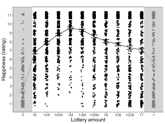
Figure 7: Expected happiness (happiness rating) as a function of the different lottery amounts (K = thousand, M = million, B = billion, T = trillion) for Study 5 (based on the within-subjects data of Block 1). Error bars represent standard errors.
Next, we analyzed the pairwise comparison data of Block 2. As in Study 4, we again used a Bradley-Terry probability model to construct a scale that numerically describes participants’ expected happiness about the different lottery amounts. We first ran an analysis in which all 12 lottery amounts were included (left panel of Figure 8), and then reran the analysis without the “no money” and the “all the money” conditions (right panel of Figure 8). In both analyses the estimated worth parameters point towards the existence of an inverted U-relation. Simonsohn’s (2018) two-line approach again formally established the existence of a general inverted U-pattern (left panel: slope of the first regression line: b = 0.03, p = .004; slope of the second regression line: b = –0.03, p = .032; right panel: slope of the first regression line: b = 0.02, p < .001; slope of the second regression line: b = –0.04, p < .001). In both analyses the breakpoint was estimated at an envisioned win of 100 million pounds.
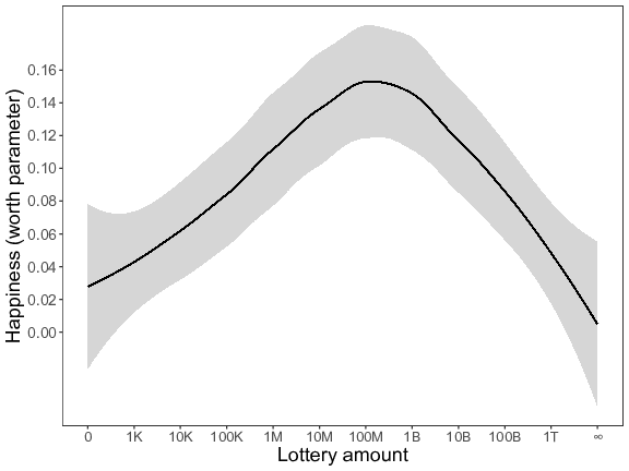
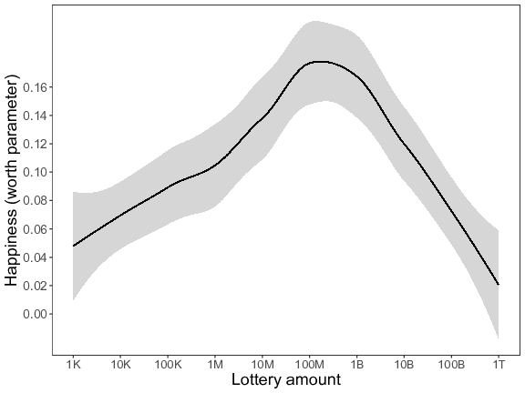
Figure 8: Expected happiness (worth parameter) as a function of the different lottery amounts (K = thousand, M = million, B = billion, T = trillion) for Study 5 (based on the pairwise comparison data of Block 2). The lines represent a loess-curve fitted to the estimated worth parameters for visualization purposes. Left panel = with all lottery amounts; right panel = without the “no money” and the “all the money” conditions.
Similar to Study 3, individual difference patterns in the within-subjects data of Block 1 were examined using the k-means function. Here too, we conducted an analysis with all lottery amounts (see left panel of Figure 9) and an analysis without the “no money ” and the “all the money” conditions (see right panel of Figure 9). In both analyses the best-fitting model contained two clusters. In Cluster 1, participants’ expected happiness ratings increased up until an amount of 10 million pounds. Then, the curve remained flat and this up until 100 billion pounds, after which the curve started to drop. In Cluster 2, the curve peaked sooner — that is, at 1 million pounds. After this point, the curve of the second cluster dropped sharply.
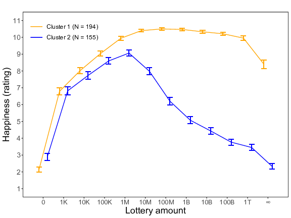
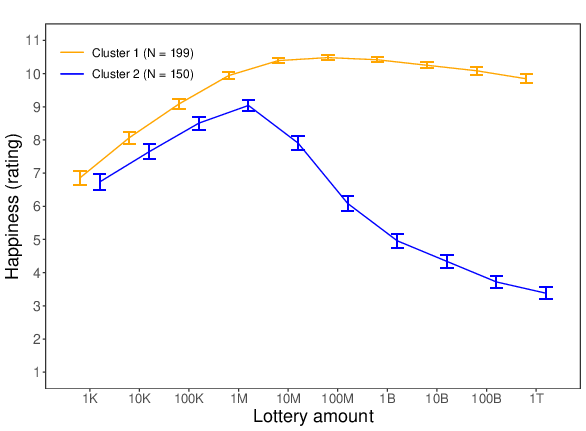
Figure 9: Two different reactions to the increasing lottery amounts (K = thousand, M = million, B = billion, T = trillion) for Study 5 (based on the within-subjects data of Block 1). Error bars represent standard errors. Left panel = with all lottery amounts; right panel = without the “no money” and the “all the money” conditions.
Similar to Study 4, individual difference patterns in the pairwise comparison data of Block 2 were investigated using the klaR package. Both the analysis with and the analysis without the “no money” and the “all the money” conditions (see, respectively, the left and the right panel of Figure 10) showed that the best-fitting model contained three clusters. In Cluster 1, expected happiness continued to rise when the amount of money that one supposedly won increased, and this up until 1 trillion pounds in the left panel and 100 billion pounds in the right panel, after which the curve in both panels decreased a bit. The curves of Clusters 2 and 3 were both characterized by an inverted V-shaped pattern. In the second cluster, the peak of the curve was reached around 1 billion pounds (in both the left and the right panel), whereas in the third cluster the curve already peaked at 10 million pounds in the left panel and at 100 thousand pounds in the right panel.
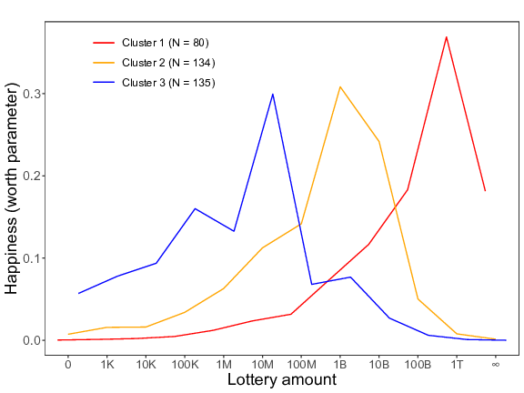
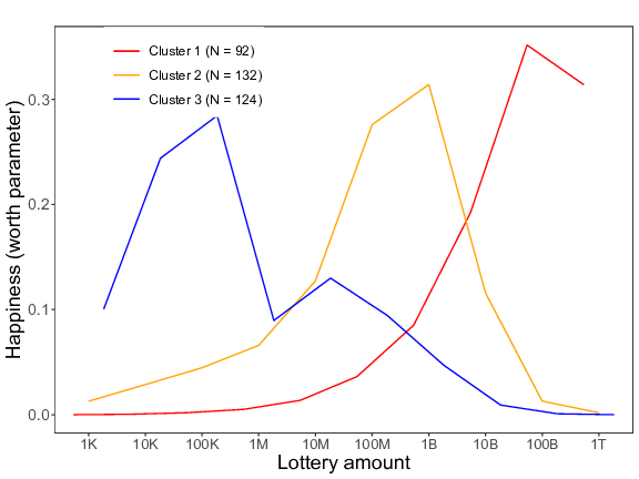
Figure 10: Three different reactions to the increasing lottery amounts (K = thousand, M = million, B = billion, T = trillion) for Study 5 (based on the pairwise comparison data of Block 2). The lines represent the estimated worth parameters of the three clusters. Left panel = with all lottery amounts; right panel = without the “no money” and the “all the money” conditions.
In the present study, the same participants were asked to evaluate the 12 different lottery amounts both separately (in Block 1) as well as in pairs (in Block 2). This particular design feature allows us to directly compare the two clusters that were extracted from the within-subjects data (Figure 9) with the three cluster that were extracted from the pairwise comparison data (Figure 10). For this comparison, we used the clusters that were extracted using all lottery amounts (left panels of Figures 9 and 10).
Table 3 illustrates that, in total, 279 of the 349 participants (79.9%) could “consistently” be categorized in one of the three clusters. More precisely, of the 194 participants of Cluster 1 in the within-subjects data, most participants belonged to either Cluster 1 (n = 75; 38.6%) or Cluster 2 (n = 94; 48.5%) in the pairwise comparison data. And, of the 155 participants of Cluster 2 in the within-subjects data, 110 participants (71.0%) belonged to Cluster 3 in the pairwise comparison data.
Table 3: Crosstabulation of the two within-subjects clusters by the three pairwise comparisons clusters (Study 5). Bold typeface denotes participants who were consistently categorized.
Pairwise comparisons clusters (Block 2) Cluster 1 Cluster 2 Cluster 3 Total Within-subjects clusters (Block 1) Cluster 1 75 94 25 194 Cluster 2 5 40 110 155 Total 80 134 135 349
In line with our expectations, these findings hence indicate that the cluster which stagnated in the within-subjects data indeed falls apart into two different clusters when using our pairwise comparisons methodology. Specifically, some of these participants (i.e., those who pertained to Cluster 1 in the pairwise comparison data) preferred the largest amounts above the intermediate amounts, whereas others (i.e., those who pertained to Cluster 2 in the pairwise comparison data) preferred the intermediate amounts above the largest amounts.
For those participants who could consistently be categorized in one of the three clusters (i.e., the ones indicated in boldface in Table 3) and who completed the follow-up part of our study, we subsequently tested for potential cluster differences. Like in Study 4, one-tailed t-tests again revealed that participants in Cluster 1 (M = 19.24, SD = 14.90) scored significantly lower on our SVO measure than those in Cluster 2 (M = 26.27, SD = 13.14, t(127) = –2.84, p = .003) and Cluster 3 (M = 30.56, SD = 10.92, t(137) = –5.16, p < .001). Here, the difference in SVO between Clusters 2 and 3 also reached statistical significance (t(158) = –2.25, p = .013). These findings thus once again illustrate that participants in Cluster 1 are more proself and less prosocially oriented than those in Clusters 2 and 3.
In order to investigate which specific prosocial and proself motivations drive participants’ responses in the three clusters, we subsequently ran a discriminant analysis (DDA). DDA is a multivariate statistical technique to compare groups for a set of continuous variables and/or to identify which variables best capture group differences (Betz, 1987; Thompson, 1998). In brief, DDA combines a set of linear covariates into K-1 composite dependent variables (i.e., the “canonical discriminant functions”), with K referring to the number of groups in the analysis (three in our case). These functions can then be evaluated to determine which variables contributed to differences between the groups (or, in other words, which variables “discriminate” best between the groups; Henson, 2000; Sherry, 2006).
We included all six motivational traits (i.e., fairness, altruism, concern for others, greed, competitiveness, and entitlement) as discriminating variables, and our three-cluster solution as the independent variable (here too, only those who were consistently categorized and who completed the follow-up part of our study were included; see above for details). This analysis yielded two canonical discriminant functions (eigenvalue Function 1 = 0.34, % explained variance = 87.4; eigenvalue Function 2 = 0.05, % explained variance = 12.6). Furthermore, there was a large canonical correlation (.50) on Function 1 with an effect size of R2 = .25, and a second, smaller canonical correlation (.21) on Function 2 with an effect size of R2 = .05. The tests of Function 1 was found to be highly significant (p < .001). The test of Function 2, however, did not reach statistical significance (p = .081), and was therefore excluded from the subsequent analyses.
We next examined the coefficients associated with Function 1 (i.e., the standardized discriminant function coefficients and structure coefficients), in order to determine which variables contributed to differences between the three clusters. In particular, the standardized coefficient associated with a variable is informative about its relative importance (i.e., it shows the “unique” contribution of that variable to the discriminant function score, similar to a regression coefficient). As shown in Table 4, for Function 1, fairness, concern for others, greed, and entitlement were primarily responsible for cluster differences, with the former two traits being negatively related.
Table 4: Standardized discriminant function and structure coefficients of the three clusters for Function 1 (Study 5).
Motivational trait Std. Coefficient r Fairness –.32 –.51 Altruism .07 –.29 Concern for others –.20 –.38 Greed .66 .82 Competitiveness .00 .45 Entitlement .37 .66 Note. Std. coefficient = standardized discriminant function coefficients. r = structure coefficients.
Finally, to determine which clusters have more (or less) of the above discriminant traits, we examined the group centroids (i.e., the mean of discriminant function scores within a group). Higher group centroids indicate that participants in that cluster display higher levels of traits that contribute positively to the relevant function and lower levels of traits that contribute negatively to the relevant function, compared to the other clusters. The results showed that, for Function 1, the group centroid of Cluster 1 is substantially higher than that of the other two clusters. More specifically, from highest to lowest centroids, the groups are Cluster 1 (.744), Cluster 2 (.215), and Cluster 3 (–.663). Comparing this to the standardized coefficients (see Table 4), it can be concluded that participants in Cluster 1 are less concerned about fairness, less concerned about others, more greedy, and feel more entitled than participants in the other two clusters, and particularly than those in Cluster 3. Although the structure coefficients indicate that altruism and competitiveness also contribute in a meaningful way to cluster differences, the standardized coefficients show that (because of their overlap with the other traits; see also the correlation matrix in Table 2) their contribution in not (largely) unique.
We started our paper with a quote attributed to Wallis Simpson, “You can never be too rich or too thin.” Most people will recognize that you can be too thin, and, as our results illustrate, many people also seem to believe that you can be too rich. Across five studies, we consistently found that, overall, the relationship between hypothetical lottery wins and expected happiness is characterized by an inverted U-shaped pattern, with the overall desired optimal lottery win being a jackpot amount of approximately 10 million pounds. Considering that in our studies participants were explicitly told that there was no upper boundary to the amount of money that they could possibly win, it can be concluded that this ‘overall’ optimum is situated at the rather low end of the continuum (and considerably lower than the global jackpot average which is situated around 29 million pounds; see Rodger, 2017). After this particular point, the overall expected happiness curve started to drop, which illustrates that, on average, the prospect of receiving too much money negatively impacts people’s overall expected happiness.
Importantly, however, is that our cluster analyses revealed that this general pattern is actually the mere mean tendency of distinct subgroups of people reacting differently to expected increases in wealth, rather than a uniform psychological reaction that is shared by all people. More specifically, our pairwise comparison data revealed the existence of a first cluster of participants (i.e., Cluster 1) who react according to the ‘more-is-better’ (non-satiation) logic. For these people, the expected happiness curve continued to rise when the amount of money that they supposedly won increased, and this even up until the highest included monetary amount of 10 billion euro (in Study 4) and 1 trillion pounds (in Study 5). So, for this type of people there does not seem to be a point of satiation (although the results of Study 5 indicate that they do not necessarily want to have “all the money in the world”). Conversely, the responses of the other two identified clusters (i.e., Clusters 2 and 3) were more in accordance with the ‘too-much-of-a-good-thing’ logic, as these participants expected to be more satisfied with the intermediate wins than with the smallest and the largest envisaged wins. So, for these types of people there is a point beyond which they anticipate that more money will negatively affect their happiness; this point was reached much sooner in the third cluster than in the second cluster. And, at very high lottery amounts the curve of the third cluster even plummeted towards the bottom of the expected happiness scale. This latter finding suggests that this particular subgroup of people does not seem to value money when it comes in great amounts, and even anticipates that this will make them quite unhappy.
Ample prior studies have demonstrated that people fundamentally differ with respect to their prosocial and proself tendencies (e.g., Au & Kwong, 2004; Bogaert el al., 2008; Van Lange, 2000). To contribute to this body of research, as a third objective, we examined if and how the clusters that could empirically be distinguished differed from each other in terms of participants’ proself and prosocial motivations. Across our studies, and in line with our expectations, we consistently found that the cluster of participants for whom there is no satiation effect (i.e., Cluster 1, which reacted according to the ‘more-is-better’ logic) is generally more proself and less prosocially oriented than the other two clusters which included participants for whom there is a point after which expected happiness decreased (i.e., Clusters 2 and 3, which reacted according to the ‘too-much-of-a-good-thing’ logic). Interestingly, our discriminant analysis clarified that the three clusters also differ in terms of more specific proself and prosocial motives. In particular, we found that participants in Cluster 1 were more greedy and also felt more entitled than those in Clusters 2 and 3, with these differences being most pronounced between Cluster 1 and Cluster 3. Furthermore, participants in Cluster 1 are not only driven more by these two specific proself motivations, they are also less concerned about fairness considerations and the welfare of others (which constitute two specific prosocial motivations).
An important strength of our work is that we collected data using a variety of research methods, including both a between-subjects design (Study 2), within-subjects designs (Studies 3 and 5), and pairwise comparisons (Studies 4 and 5). The fact that we could replicate our key findings using this divergence in methods and designs strengthens our confidence in the robustness and generalizability of the reported findings. Yet, our approach to employ hypothetical lottery scenarios also contains two important constraints. First, because the lottery wins in our studies were imagined, participants did not really experience the surprise of receiving the message or actually using the money. Instead, they formed a mental model of what they believed would happen. Secondly, lottery wins are a windfall gain whereas other sources of wealth often have a strong link to meritocracy (or at least the illusion of it). In this vein, Donnelly et al. (2018) have shown that earned wealth is associated with greater happiness than inherited wealth.
Although we found some interesting motivational differences between the three emerging clusters, we did not consider all relevant motivational traits and personality factors in our research. A first important motivation that we did not consider in any of our studies is inequality aversion. Given that lotteries by their nature increase inequality, this concept might be particularly relevant to consider in future studies. Another important personality factor that was not included in the present research is the Honesty-Humility dimension of the HEXACO model (Hilbig & Zettler, 2009), which specifically contains a facet called greed avoidance. Low scorers on this trait want to enjoy and display wealth and privilege, whereas high scorers are not especially motivated by monetary or social-status considerations. In light of our research, it can be expected that those whose reactions are in accordance with the ‘too-much-of-a-good thing’ logic (i.e., Clusters 2 and 3) will score higher on inequality aversion and greed avoidance than those whose reactions endorse the ‘more-is-better’ logic (i.e., Cluster 1), but future research is needed to verify these claims.
The empirical evidence presented in the present paper sheds new light on the question if people believe that money will buy them happiness, and whether they think that more money also leads to greater happiness. Our mental simulation experiments show that, generally speaking, people indeed believe that money and happiness are positively connected. Critically, however, our research also illustrates that there is a clear upper limit to most people’s general desire for money, and that a substantial part of the population even anticipates that having too much money will make them less happy. Excesses in everyday life are not always wonderful, and money does not seem to be an exception in this respect, at least in many people’s perception.
Au, W. & Kwong, J. (2004). Measurements and effects of social-value orientation in social dilemmas: A review. In R. Suleiman, D. Budescu, I. Fischer, & D. Messick, (Eds.), Contemporary Psychological Research on Social Dilemmas (pp. 71-98). New York: Cambridge University Press
Betz, N. E. (1987). Use of discriminant analysis in counseling psychology research. Journal of Counseling Psychology, 34, 393–403.
Bogaert, S., Boone, C., & Declerck, C. (2008). Social value orientation and cooperation in social dilemmas: A review and conceptual model. British Journal of Social Psychology, 47, 453-480.
Brickman, P., Coates, D., & Janoff-Bulman, R. (1978). Lottery winners and accident victims: Is happiness relative? Journal of Personality and Social Psychology, 36, 917–927.
Brue, S. L. (1993). Retrospectives: The law of diminishing returns. Journal of Economic Perspectives, 7, 185–192.
Campbell, W. K., Bonacci, A. M., Shelton, J., Exline, J. J., & Bushman, B. J. (2004). Psychological entitlement: Interpersonal consequences and validation of a self-report measure.
Dittrich, R., Hatzinger, R., & Katzenbeisser, W. (1998). Modelling the effect of subject-specific covariates in paired comparison studies with an application to university rankings. Journal of the Royal Statistical Society: Series C (Applied Statistics), 47, 511–525.
Donnelly, G. E., Zheng, T., Haisley, E., & Norton, M. I. (2018). The amount and source of millionaires’ wealth (moderately) predict their happiness. Personality and Social Psychology Bulletin, 44, 684-699.
Grant, A. M., & Schwartz, B. (2011). Too much of a good thing: The challenge and opportunity of the inverted U. Perspectives on Psychological Science, 6, 61–76.
Haesevoets, T., Van Hiel, A., Van Assche, J., Bostyn, D., & Reinders Folmer, C. (2019). An exploration of the motivational basis of take-some and give-some games. Judgment and Decision Making, 14, 535–546.
Hatzinger, R., & Dittrich, R. (2012). Prefmod: An R package for modeling preferences based on paired comparisons, rankings, or ratings. Journal of Statistical Software, 48, 1–31.
Henson, R. K. (2000). Demystifying parametric analyses: Illustrating canonical correlation as the multivariate general linear model. Multiple Linear Regression Viewpoints, 26, 11–19.
Hilbig, B. E., & Zettler, I. (2009). Pillars of cooperation: Honesty–Humility, social value orientations, and economic behavior. Journal of Research in Personality, 43, 516-519.
Hsee, C. K. (1996). The evaluability hypothesis: An explanation for preference reversals between joint and separate evaluations of alternatives. Organizational Behavior and Human Decision Processes, 67, 247–257.
Hsee, C. K., Loewenstein, G. F., White, S. B., & Bazerman, M. H. (1999). Preference reversals between joint and separate evaluations of options: A review and theoretical analysis. Psychological Bulletin, 125, 576-590.
Hsee, C. K., & Zhang, J. (2010). General evaluability theory. Perspectives on Psychological Science, 5, 343–355.
Huang, Z. (1997). A fast clustering algorithm to cluster very large categorical data sets in data mining. Dmkd, 3, 34–39.
Krekels, G., & Pandelaere, M. (2015). Dispositional greed. Personality and Individual Differences, 74, 225–230.
Kuhlman, D. M., & Marshello, A. (1975). Individual differences in game motivation as moderators of preprogrammed strategy effects in prisoner’s dilemma. Journal of Personality and Social Psychology, 32, 922-931.
Lindqvist, E., Östling, R., & Cesarini, D. (2020). Long-run effects of lottery wealth on psychological well-being. The Review of Economic Studies, 87, 2703–2726.
Lu, S., Au, W., Jiang, F., Xie, X., & Yam, P. (2013). Cooperativeness and competitiveness as two distinct constructs: Validating the Cooperative and Competitive Personality Scale in a social dilemma context. International Journal of Psychology, 48, 1135–1147.
Lutter, M. (2007). Book Review: Winning a lottery brings no happiness! Journal of Happiness Studies, 8, 155–160.
MacQueen, J. (1967). Classification and analysis of multivariate observations. In 5th Berkeley Symp. Math. Statist. Probability (pp. 281-297).
McClintock, C. G., & Liebrand, W. B. G. (1988). The role of interdependence structure, individual value orientation and other’s strategy in social decision making: A transformational analysis. Journal of Personality and Social Psychology, 55, 396–409.
Meade, A. W., & Craig, S. B. (2012). Identifying careless responses in survey data. Psychological methods, 17, 437–455.
Messick, D. M., & McClintock, C. G. (1968). Motivational bases of choice in experimental games. Journal of Experimental Social Psychology, 4, 1–25.
Murphy, R. O., Ackermann, K. A., & Handgraaf, M. (2011). Measuring social value orientation. Judgment and Decision making, 6, 771-781.
Nisslé, S., & Bschor, T. (2002). Winning the jackpot and depression: Money cannot buy happiness. International Journal of Psychiatry in Clinical Practice, 6, 183–186.
Oswald, A. J., & Winkelmann, R. (2019). Lottery Wins and Satisfaction: Overturning Brickman in Modern Longitudinal Data on Germany. In Rojas M. (Ed), The Economics of Happiness (pp 57-84). Springer, Cham.
Raschke, C. (2019). Unexpected windfalls, education, and mental health: Evidence from lottery winners in Germany. Applied Economics, 51, 207–218.
Rodger, J. (2017). This is how much the average lottery win is in each country. https://www.coventrytelegraph.net/news/coventry-news/how-much-average-lottery-win-13218034.
Sharif, M. A., Mogilner, C., & Hershfield, H. E. (2021). Having too little or too much time is linked to lower subjective well-being. Journal of Personality and Social Psychology, 121, 933–947.
Sherry, A. (2006). Discriminant analysis in counseling psychology research. The Counseling Psychologist, 34, 661–683.
Selenta, C., & Lord, R. G. (2005). Development of the levels of self-concept scale: Measuring the individual, relational, and collective levels. Working paper, University of Akron.
Seligman, M. E., & Csikszentmihalyi, M. (2014). Positive psychology: An introduction. In Flow and the foundations of positive psychology (pp. 279-298). Springer, Dordrecht.
Simonsohn, U. (2018). Two lines: A valid alternative to the invalid testing of U-shaped relationships with quadratic regressions. Advances in Methods and Practices in Psychological Science, 1, 538–555.
Sinclair C. D. (1982). GLIM for Preference. In R. Gilchrist (ed.), Proceedings of the International Conference on Generalised Linear Models (pp. 164-178). New York: Springer-Verlag.
Smith, V. L. (1976). Experimental economics: Induced value theory. The American Economic Review, 66, 274–279.
Stevenson, B., & Wolfers, J. (2013). Subjective well-being and income: Is there any evidence of satiation? American Economic Review, 103, 598-604.
Tazelaar, M. J. A., Van Lange, P. A. M., & Ouwerkerk, J. W. (2004). How to cope with “noise” in social dilemmas: the benefits of communication. Journal of Personality and Social Psychology, 87, 845–859.
Thompson, B. (1998, April). Five methodological errors in educational research: The pantheon of statistical significance and other faux pas. Invited address presented at the annual meeting of the American Educational Research Association, San Diego, CA.
Tibshirani, R., Walther, G., & Hastie, T. (2001). Estimating the number of clusters in a data set via the gap statistic. Journal of the Royal Statistical Society: Series B (Statistical Methodology), 63, 411-423.
Van Hiel, A., Vanneste, S., & De Cremer, D. (2008). Why did they claim too much? The role of causal attributions in explaining level of cooperation in commons and anticommons dilemmas. Journal of Applied Social Psychology, 38, 173–197.
Van Lange, P. A. (1999). The pursuit of joint outcomes and equality in outcomes: an integrative model of social value orientation. Journal of Personality and Social Psychology, 77, 337–349.
Van Lange, P. A. M. (2000). Beyond self-interest: A set of propositions relevant to interpersonal orientations. In W. Stroebe & M. Hewstone (Eds.), European review of social psychology (Vol. 11, pp. 297-331). New York: Wiley.
Van Lange, P. A. M., & Kuhlman, D. M. (1994). Social value orientations and impressions of partner’s honesty and intelligence: A test of the might versus morality effect. Journal of Personality and Social Psychology, 67, 126-141.
Weihs, C., Ligges, U., Luebke, K. and Raabe, N. (2005). klaR Analyzing German Business Cycles. In Baier, D., Decker, R. and Schmidt-Thieme, L. (Eds.), Data Analysis and Decision Support (pp. 335-343). Springer-Verlag, Berlin.
Data transparency: The data and data analysis scripts of our studies are made publicly available and can be accessed through the following OSF webpage: https://osf.io/j9sxa.
Funding information: This research was supported by Grant BOF.PDO.2017.0017.01 of the Special Research Fund (Bijzonder Onderzoeksfonds) of Ghent University.
Acknowledgement: The authors would like to thank Emiel Van Den Eynden for his help with the data collection of Study 4.
Copyright: © 2022. The authors license this article under the terms of the Creative Commons Attribution 4.0 License.
This document was translated from LATEX by HEVEA.