Judgment and Decision Making, Vol. 17, No. 6, November 2022, pp. 1287-1312
Value-directed information search in partner choice
Hongyi Wang*
Jiaxin Ma#
Lisheng He$ |
Abstract: It is a widely held view that people rely on incomplete information to find a relationship partner, resulting in non-compensatory choice heuristics. However, recent experimental work typically finds that partner choice follows compensatory choice strategies. To bridge this gap between theory and experimental evidence, we characterize the mate choice problem by distinguishing the information search process from the evaluation process. In an eye-tracking experiment and a MouseLab experiment, we show that people display strong value-directed search heuristics in response to all types of cues and that the magnitude of value-directed searches increases with cue primacy. Cue primacy also explains the interaction effect of cue type and participant sex on the extent of valued-directed search. We further argue that value-directed searching does not necessarily lead to non-compensatory choice rules but may serve compensatory decision-making. Our results demonstrate that people may adopt remarkably smart search heuristics to find an ideal partner efficiently.
Keywords: information search, partner choice, cue primacy, process tracing, computational modeling.
1 Introduction
Finding the right person as a relationship partner is one of the most important decisions grown-ups make in life. Partner selection is difficult. In general terms, it can be described as a large-scale bipartite game in which intra-sexual members compete to get their desirable partners, obtaining from the relationship entities such as good genes, financial resources, social status, and a good intra-relationship match (Buss & Schmitt, 1993; Chiappori, 2020; Dupuy & Galichon, 2014; Gale & Shapley, 1962; Miller & Todd, 1998). Quite apart from the bipartite strategic dynamics, the preferential partner choice is not necessarily easy. We have many opportunities to interact with others to evaluate their mate values and eventually find a desirable partner. People use various cues such as facial attractiveness, financial resources, social status, intelligence, and resemblance to themselves to form mate values (see Buss et al., 2001 for a review). The acquisition of information requires a sequential search involving asking questions, conversing, and interacting with the person, or at least looking at the person to judge how good-looking they are. Considering the vast number of potential candidates and cues, as well as the financial and cognitive costs involved in information search, it would, therefore, be maladaptive to evaluate all possible candidates and cues for a complete evaluation (Miller & Todd, 1998).
In response, researchers have proposed that people use cognitive shortcuts to make efficient information searches, guiding subsequent choices (Lenton et al., 2013; Miller & Todd, 1998). The sequential aspiration model, for example, assumes that people assess the values of potential candidates sequentially and pursue further courtship only if the potential candidates’ trait value exceeds the aspiration level. Such features are built into online dating apps that present only a primary cue (in most cases, a profile photo that displays a person’s physical appearance) and do not disclose further information until the primary cue meets a certain threshold. Similarly, heuristic models, such as take-the-best, assess the cues in the order of importance and stop when one option exceeds others on one cue, which may result in non-compensatory choice behavior that may violate normative principles of rational choice such as transitivity (Gigerenzer & Goldstein, 1996; Miller & Todd, 1998).
However, the evidence for non-compensatory strategies for mate choice is lacking in experimental research. Instead, recent studies suggest that human and nonhuman mate preferences rarely violate rational choice axioms such as transitivity (Arbuthnott et al., 2017; Dechaume-Moncharmont et al., 2013; Wang et al., 2021). Furthermore, mate choice data are better described by compensatory strategies (e.g., weighted additive model, Euclidean distant model) than non-compensatory heuristic strategies (e.g., sequential aspiration model, take-the-best) (Brandner et al., 2020; Conroy-Beam, 2018). Brandner et al. (2020), for example, made a comprehensive comparison of different models using different numbers of cues and found consistent evidence that supports the compensatory view of mate choice. Those results stand in stark contrast with the widely held view of heuristic mate choice behavior.
In this study, we reconcile this conflict by distinguishing the information search process from the evaluation process in the mate choice problem, drawing upon research on the cognitive processes of human decision-making (Jekel et al., 2018; Payne et al., 1993). Recent advances in cognitive science suggest that people display value-directed search tendencies in which more information about high-value options is collected in the decision processes (e.g., Gluth et al., 2020). Furthermore, such a value-directed search does not necessarily lead to suboptimal choices. In fact, it has been argued that value-directed search is the product of efficient allocation of attention when the decision-maker needs to learn about the value of the options from the acquired information (Callaway et al., 2021; Jang et al., 2021). The intuition is as follows: In choosing the highest-value option, decision-makers do not need to reveal the value of all options, as they only need to find the one with the highest value. Therefore, the decision-maker should prioritize information acquisition from high-value options and rationally undersearch low-value options (Callaway et al., 2021; Sepulveda et al., 2020). Closer to home, our idea is closely related to the influential sequential aspiration model (Miller & Todd, 1998), and can be seen as an implementation of the model regarding information gathering for mate choice.
We hypothesize that observing a high cue value (e.g., an attractive face) in a candidate would increase the chance of searching for other cues in the same candidate. Similar value-directed search patterns have been observed in other choice tasks. For example, in risky choice, observing a high probability increases the likelihood of fixating on its associated payoffs (Fiedler & Glöckner, 2012). In hotel choice, observing a high cleanliness rating increases the likelihood of searching for price information (Jekel et al., 2018; Scharf et al., 2019). Therefore, we expect to observe similar patterns in mate choice. That is, observing a high cue value in a candidate makes the decision maker more likely to search for more information about the candidate under evaluation.
The value-directed search would also depend on cue primacy because diagnostic cues contribute more to the mate value than non-diagnostic ones. Men typically weigh physical attractiveness more heavily than women do, while women tend to weigh financial resources and intelligence more heavily than men do (Buss, 1989; Buss & Barnes, 1986). Such sex differences are highly robust across studies, although the origin of the sex differences in cue primacy remains debatable (Eagly & Wood, 1999; Kenrick et al., 1993). Therefore, we further hypothesize that men would display a stronger value-directed search in response to facial attractiveness than women would and that women would display a stronger value-directed search in response to resource- or intelligence-related cues than men would.
We tested our hypotheses in two process-tracing experiments that tracked participants’ information search processes while they were making partner choice. Experiment 1 was an eye-tracking experiment, during which participants were asked to choose between two candidates using two cues, face and monthly income. Experiment 2 was a MouseLab experiment, where participants chose one from six candidates varying in three cues: face, monthly income, and creativity. Over the two experiments with varying numbers of options and cues, participants reliably displayed the hypothesized value-directed information search for partner choice.
2 Experiment 1: Eye-tracking
2.1 Methods
Participants. Fifty-eight heterosexual women (mean age = 21.60 years, SD = 2.22) and 49 heterosexual men (mean age = 21.67 years, SD = 2.38) participated in the study. All the participants were college students at a university in China, and all reported normal or corrected-to-normal vision. All participants received a flat payment of 20 CNY. The study was conducted in accordance with the Declaration of Helsinki and was approved by the Committee of Human Research Protection at a university in China.
Stimuli. We created two sets of profiles. One set consisted of 18 male profiles (for female participants), and the other set consisted of 18 female profiles (for male participants). Each profile contained information on two cues: physical attractiveness and financial resources (indicated by monthly income). Following previous studies, we used face images to convey physical attractiveness (e.g., Brandner et al., 2020; Wang et al., 2021). We created 153 pairs of profiles by exhausting all pairwise combinations from the 18 profiles in each set.
The 36 profiles were created as follows. The face images were scraped from an open online employee database of a brokerage company (www.lianjia.com). All face images were anonymized portrait photos displayed in 300px × 400px ellipses. To obtain face images that spanned different attractiveness levels, we recruited an independent group of participants (15 heterosexual men and 15 heterosexual women) to rate the perceived attractiveness of opposite-sex face images. Eighteen male face images and 18 female face images were selected based on the average attractiveness ratings, such that female and male face images are similar in the mean and standard deviation of the rated attractiveness. The monthly income for each profile was randomly generated from a uniform distribution between 6,000 CNY and 25,000 CNY. We set the monthly income in the middle range, without extremely high or low values. At the time of the experiment, 1,000 CNY was worth approximately 157 USD.
Procedures. Participants were seated approximately 70 cm from a 23-inch screen with a resolution of 1920 × 1200 pixels. Before the experiment started, they could adjust the seat height to make themselves comfortable while looking at the screen before the experiment began. After that, we asked them to remain seated as still as possible throughout the experiment. Eye movements were recorded using a Tobii TX300 Eye Tracker at a sample rate of 300 Hz. A nine-point eye calibration was performed at the beginning of the experiment to ensure the precision of eye tracking.
Participants were then instructed to imagine that they were browsing online dating profiles and making binary choices in pairs of potential romantic partners’ profiles. Each trial began with a fixation cross at the center of the screen for 500ms, followed by two profiles on display, one on the left side and the other on the right side of the screen (Figure 1). In each trial, we presented the participants with one pair of profiles. The two profiles were horizontally aligned and displayed either on the left or right side of the screen at random. The face images were placed at the upper corners, and the monthly incomes were placed at the lower corners of the screen. The placement order was held constant across trials. Participants were allowed to view the profiles in a self-paced manner until a choice was made by pressing either F or J on the keyboard (pressing “F” selected the left profile and pressing “J” selected the right one). The order of the 153 trials was randomized across participants.

| Figure 1: Illustration of the trials in Experiment 1. Each trial was a binary choice between two profiles varying on two cues: facial attractiveness and monthly income. Facial attractiveness was indicated by the profile photos at the upper corners, while the income was displayed using bars and Arabic numbers at the lower corners of the screen. Participants pressed “F” to choose the left profile, and “J” to choose the right profile. In the figure, the profile photos have been replaced by abstract symbols for privacy and copyright reasons. |
Following the choice tasks, participants rated all the faces on attractiveness using a 9-point scale. We did not record eye movements during the rating task.
Data pre-processing. To analyze the eye-tracking data, we created four areas of interest (AOIs) corresponding to Left Face, Left Income, Right Face, and Right Income, respectively. We used circles with a radius of 378px as the AOIs. We chose this radius because it made the AOIs tangential to one another, obtaining the largest number of valid fixations in the eye-gaze data. Eye fixations outside of the AOIs were excluded from the subsequent eye-gaze data analysis. Trials that yielded less than two valid fixations were excluded, as no transitions were available. The data from one participant were excluded because of a low gaze sample rate (< 50%, meaning that the eye tracker captured less than half of the gaze data for this participant). After pre-processing, we were left with 15,504 trials from 106 participants.
Choice models. We used the compensatory weighted additive (WADD) choice model to evaluate the extent to which the different cues determined partner choice and how that extent differed between men and women. The main weighted additive choice model, WADDFull, took both cues into consideration:
|
| |
Pr[Left|Left, Right]j = L
| ⎛
⎝ |
α1 Δ attrj + α2 Δ incomej + α3 Δ attrj · sex + α4 Δ incomej · sex
| ⎞
⎠ |
|
(1) |
where L(·) is the logistic transformation. Δ attrj denotes the difference in attractiveness between the left and right profiles in trial j using the participant’s own ratings. A positive Δ attrj indicates that the left profile was more attractive than the right profile. Δ incomej denotes the difference in monthly income between the two profiles in trial j. A positive Δ incomej indicates that the left profile had a higher income than the right profile. Δ attrj and Δ incomej were both standardized in the models. sex∈ {−0.5,0.5} denotes participant sex, where sex=−0.5 indicates a woman participant, and sex=0.5 indicates a man.
In two additional weighted additive models, we used one of the two cues for choice predictions, respectively. In WADDAttractiveness, we only used the rated attractiveness to predict partner choice and thus turned off α2 and α4 in the model. In WADDIncome, we only used the monthly income to predict partner choice and thus turned off α1 and α3.
We fitted the WADD models using the hierarchical Bayesian method in rstanarm (Goodrich et al., 2020). In the hierarchical Bayesian model fits, α1 and α2 were allowed to vary across participants whereas α3 and α4 were held constant across participants, as participant sex was a between-subject factor. The priors were set as default (i.e., standard normal). For each fit, we drew four independent chains each containing 5,000 formal iterations after 5,000 burn-in iterations, totaling 20,000 formal iterations. In the paper, we report posterior mean and 95% credible intervals (95% CIs) of the parameters in the hierarchical Bayesian fit, unless otherwise specified.
Markov search model of eye movement. We used a Markov search model to characterize the value-directed search dynamics, while rigorously controlling for other search tendencies. The model predicted the switches between the four AOIs (denoted by S) using transition probabilities Pr[st|st−1], where st−1, st ∈ S and t = 2,3,...,T are the time steps. We further wrote Pr[st|st−1] as a function of the following sets of predictor variables:
|
| |
Pr[st|st−1]= σ
| ⎛
⎝ |
β1 BtOpt + β2 BtCue + β3 ItFaceSameOpt + β4 ItIncomeSameOpt + (β5 ItFaceSameOpt + β6 ItIncomeSameOpt) · zt−1 + sex · (β7 BtOpt + β8 BtCue) + sex · (β9 ItFaceSameOpt + β10 ItIncomeSameOpt) + sex · (β11 ItFaceSameOpt + β12 ItIncomeSameOpt)· zt−1
| ⎞
⎠ |
|
(2) |
where σ(·) is the softmax function such that ∑st ∈ SPr[st|st−1] = 1.
In Line 1 of Eq. 2, BtOpt denotes whether st was in the left or right option (0 = Left, 1 = Right) and BtCue denotes whether st was a face or an income cue (0 = Income, 1=Face). Therefore, β1 describes the search bias toward the right option (versus the left option) and β2 describe the search bias toward the faces (versus the income information).
In Line 2, ItFaceSameOpt indicates whether st−1 was a face cue and st and st−1 belonged to the same option (1 = yes, 0 = no), whereas IIncomeSameOpt indicates whether st−1 was an income cue and st and st−1 belonged to the same option (1 = yes, 0 = no). Correspondingly, β3 describes the extent of within-option search after observing a face cue, and β4 describes the extent of within-option search after observing an income cue.
In Line 3, zt−1 stands for the revealed cue value in step st−1. We standardized the raw values within each cue into z-scores to make the values of facial attractiveness and monthly income comparable. Therefore, β5 captures the extent to which the observed facial attractiveness determines subsequent within-option switches, and β6 captures the extent to which the observed monthly income determines subsequent within-option switches.
Lines 4 to 6 capture the sex differences in the various eye movement tendencies. The three lines correspond to Lines 1–3 respectively. sex indicates whether the participant was a man (sex=0.5) or a woman (sex=−0.5). As sex is a between-participant variable, β7 through β12 in the three lines were held constant across participants (i.e., no individual-level variation was allowed) in the hierarchical Bayesian model fitting.
We also specified starting point probabilities using: Pr[s1|s0] = σ((β1 + β7 · sex)B1Opt + (β2 + β8 · sex)B1Cue), where s0 represents the start of a trial. This specification allowed the first searched state s1 in each trial to depend on the right-side search bias in β1 and the face cue search bias in β2, as well as the corresponding sex differences in β7 and β8.
We fitted the model using the hierarchical Bayesian method in rstan (Stan Development Team, 2021). The hyperprior of the group-level parameters was set as the standard normal distribution. For each of the parameters, we needed to specify the dispersion of individuals’ deviation from the group-level mean σk and used a half-Cauchy distribution (with location = 0 and scale = 5) as the prior specification such that σk ≥ 0. We allowed participants to have different values for parameters β1 through β6 in Eq. 2, as in a typical hierarchical Bayesian analysis. We ran four independent chains, each consisting of 2,500 formal iterations after 1,000 burn-in iterations, totaling 10,000 formal iterations for the posterior approximation. All Rubin-Gelman R values were below 1.05, indicating excellent convergence of the MCMC simulation (Gelman & Rubin, 1992).
Open Practices Statement. The data and code for Experiment 1 are available at the associated OSF repository: https://osf.io/pzxgd/. None of the analyses in Experiment 1 was formally preregistered.
2.2 Results
Data summary. Participants, on average, chose 52.2% of the left profiles across all trials. A mixed-effect logistic regression model suggested a small but significant left bias in choice data (z = 5.49, p < 10−7). In each trial, participants made an average of 9.38 fixations on the four AOIs, as defined in the Methods section. Of the fixations, 49.4% were on the left profile, and 72.% were on the face cues.
In attractiveness ratings, female face images and male face images were rated as equally attractive (Mfemale = 4.83, Mmale = 4.67; t34 = 0.36, p = .72). Furthermore, the standard deviation of the rated attractiveness of female and male profile photos were comparable (SDfemale = 1.39 versus SDmale = 1.43). Since heterosexual female and male participants were only treated with opposite-sex profiles, the similarity in the rated attractiveness of female and male face images was important for comparing sex differences in the role of facial attractiveness in information search and decision making.
In eye-movement data, women gazed at faces 69.7% of the time, while men gazed at faces 75.7% of the time (t103.5 = 3.32, p = .001), suggesting that men devoted more attention to acquiring facial information than women did. This result was consistent with the choice data below that revealed that facial attractiveness was more diagnostic in men’s choices than in women’s.
Cue primacy in choice data. The hierarchical Bayesian estimation of WADDFull examined the extent to which facial attractiveness and monthly income of the profiles determined partner choices (see Table 1). In line with the large body of literature, attractiveness and income strongly predicted partner choice (α1, α2 > 0). We also observed a strong interaction between participant sex and attractiveness , suggesting that men’s choices were more strongly determined by the perceived attractiveness than women’s choices were (α3 > 0). While women chose the more attractive profile 68% of the time, men chose 81% of the more attractive profile in binary choices. No interaction between participant sex and income was observed (α4).
| Table 1: Hierarchical Bayesian estimation of the full weighted additive choice model in Experiment 1 (Equation 1). |
| 2*Parameter | 2*Interpretation | Posterior estimation |
| | | Mean | 95% CI |
| α1 | Attractiveness | 1.20 | [0.98, 1.43] |
| α2 | Income | 1.63 | [1.24, 2.03] |
| α3 | Sex × Attractiveness | 2.08 | [1.71, 2.46] |
| α4 | Sex × Income | 0.29 | [-0.31, 0.87] |
To further determine the relative cue primacy of facial attractiveness and income, we used two additional weighted additive models to predict participants’ choice data, and evaluated their predictive accuracy. In WADDAttractiveness, only facial attractiveness was used for choice predictions, whereas in WADDIncome, only monthly income was used for choice predictions. We found that WADDAttractiveness predicted choice data more accurately than WADDIncome did, with a log Bayes factor (using natural base) margin of 253 (Kass & Raftery, 1995). Both models performed substantially worse than the full model WADDFull, with log Bayes factor (using natural base) margins of 2127 and 1874 respectively. Therefore, although both cues contributed to the final decisions, facial attractiveness emerged as a more important cue in partner selection than financial income in the experiment.
Interactive search dynamics. Our main prediction was the value-directed interactive search and that the value-directed interactive search dynamics differed across cues and participant sexes depending on cue primacy. To test these, we correlated the perceived attractiveness with the transition probability to the income information in the same option, separately for men and women to test how the perceived attractiveness influenced subsequent within-option information sampling. As Figure 2 shows, we found that an attractive face led to increased transitions to its corresponding income information for both men and women and that this pattern appeared to be stronger in men than in women (men: r = 0.83, p = .005; women: r = 0.44, p = 0.240). Note that the face-to-income within-option transitions were relatively infrequent for both sexes, with transition probabilities below the baseline level of 0.25. This was likely because income was a less important cue for partner choice, and was less often attended to, than the faces in the experiment.
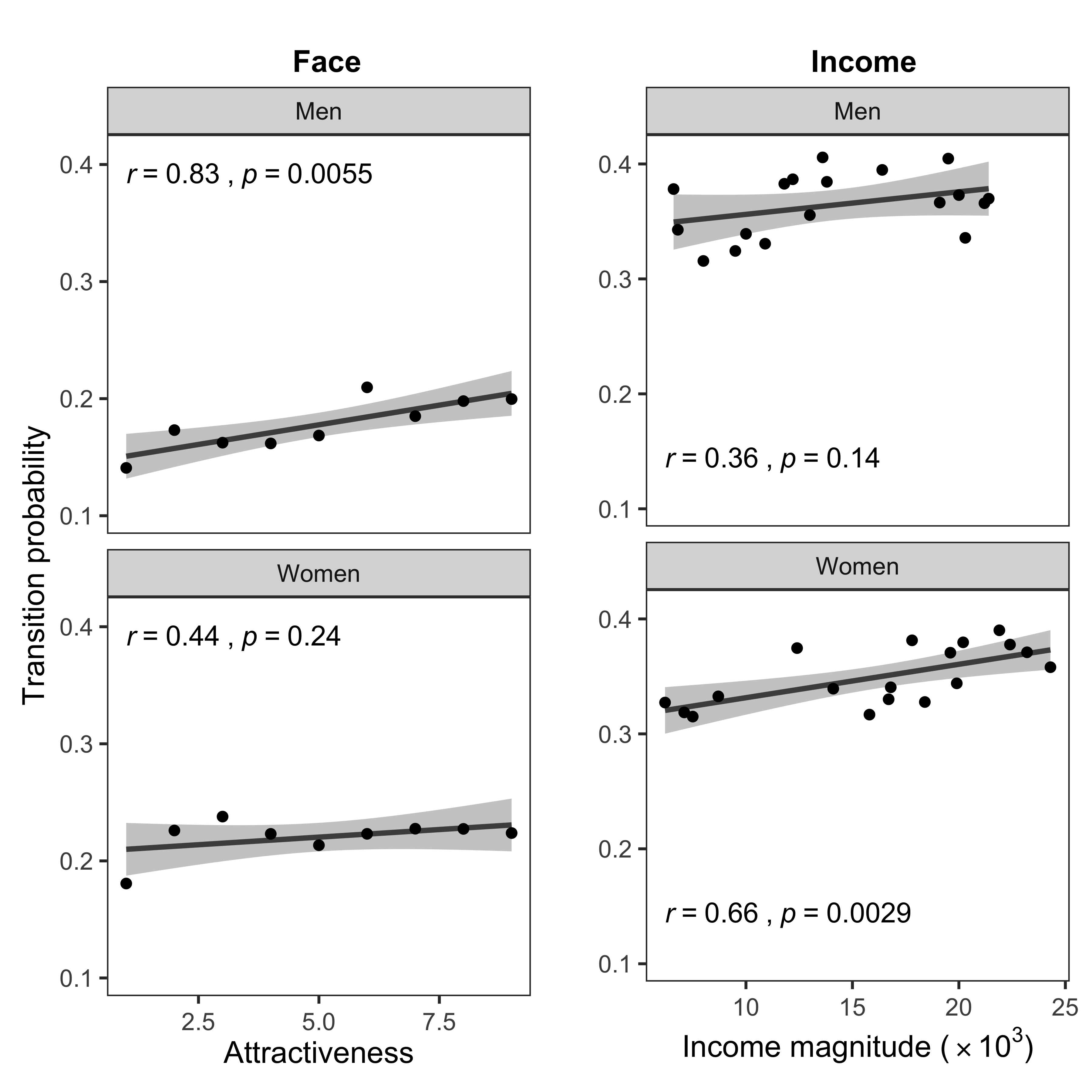
| Figure 2: Interactive search dynamics in Experiment 1. Group-level correlations between cue desirability and subsequent within-option transition probabilities, separately for men and women. |
Similarly, we tested whether observing a high income led to increased transition probabilities to the corresponding profile’s face. This effect existed in men and women and appeared to be stronger in women than in men (men: r = 0.36, p = .14; women: r = 0.66, p = .003). The income-to-face within-option transitions were more likely than the reverse, This was likely due to the fact that faces were fixated on much more often than the income information in the experiment.
We tested these patterns more rigorously, using a Markov search model characterizing the interactive search while controlling for a number of search tendencies. We fitted the model to eye-gaze data in a hierarchical Bayesian framework (see Table 2 for a summary of group-level parameters). In aggregate, participants showed substantial face-to-income interactive search (β5 > 0), whereby high facial attractiveness led to more transitions to the income in the same profile, and income-to-face interactive search (β6 > 0), whereby high income led to more transitions to the face in the same profile. A comparison of the two directions of interactive search suggested that the overall face-to-income interactive search was stronger than the reverse (β5 − β6 = 0.04, 95% CI = [0.003, 0.08]). Additionally, according to Table 2, participants in Experiment 1 were slightly tilted towards searching for the right profiles ( β1> 0), were far more likely to search for the facial than the income information ( β2 > 0), and displayed strong within-option transitions in response to both types of cues ( β3,β4 > 0).
In the Markov search model, we also tested sex differences in the interactive search dynamics. We found that men made more face-to-income interactive search than women did (β11 > 0), but men and women did not differ substantially in the reverse direction (i.e., 95% CI of β12 contains zero). There were also sex differences regarding other search tendencies. For example, men displayed more right-side search bias (β7 > 0), allocated more attention toward faces (β8 > 0), and made fewer within-option transitions (β9, β10 < 0) than women did.
| Table 2: Hierarchical Bayesian estimation of the Markov search model in Experiment 1 (Equation 2). |
| 2*Parameter | 2*Interpretation | Posterior estimation |
|
| | Mean | 95% CI |
| β1 | Right bias | 0.03 | [0.00, 0.05] |
| β2 | Cue bias | 1.05 | [0.95, 1.14] |
| β3 | FaceSameOption | 0.81 | [0.75, 0.87] |
| β4 | IncomeSameOption | 0.43 | [0.37, 0.49] |
| β5 | FaceSameOption×Attractiveness | 0.14 | [0.12, 0.16] |
| β6 | IncomeSameOption×Magnitude | 0.10 | [0.07, 0.13] |
| β7 | Sex×Right | 0.10 | [0.05, 0.15] |
| β8 | Sex×Cue | 0.32 | [0.12, 0.51] |
| β9 | Sex×FaceSameOption | -0.23 | [-0.35, -0.12] |
| β10 | Sex×IncomeSameOption | -0.12 | [-0.24, -0.00] |
| β11 | Sex×FaceSameOption×Attractiveness | 0.10 | [0.06, 0.13] |
| β12 | Sex×IncomeSameOption×Magnitude | -0.01 | [-0.08, 0.05] |
2.3 Discussion
In Experiment 1, the participants exhibited extensive value-directed interactive search, and the extent of interactive search depends on cue primacy. The between-sex asymmetry in interactive search was consistent with the adaptive information search with the goal to find a high-value person. As shown above, although both men and women treat attractiveness as the primary attribute, women relies slightly less on attractiveness in mate choice. Correspondingly, revealing an attractive face image (via gazing at the face) is particularly informative for men seeking to find a high-value person and therefore leading to more within-option transitions to the income information.
Note that the overall face-to-income within-option transition probabilities were lower than the income-to-face within-option transition probabilities. That was likely because the participants paid a disproportionate amount of attention to faces and thus the overall attention probabilities to the income information are relatively low. Nonetheless, we observed the predicted interactive search dynamics in both directions. The Markov search model further allows us to measure the extent of the interactive search in a principled yet tractable manner.
3 Experiment 2: MouseLab
In Experiment 2, we used the MouseLab paradigm to accommodate more cues and more profiles in the search-and-choice task (Willemsen & Johnson, 2011). Here, participants chose one from six candidates varying in three cues: facial attractiveness, monthly income, and creativity.
3.1 Methods
Participants. Fifty heterosexual women (mean age = 21.64 years, SD = 1.71) and 54 heterosexual men (mean age = 21.70 years, SD = 1.91) participated in the study. All the participants were university students recruited via online advertisements and received a flat payment of 20 CNY after finishing the experiment. The study was conducted in accordance with the Declaration of Helsinki and was approved by the Committee of Human Research Protection at a university in China.
Stimuli. We created two sets of profiles, one set of male profiles for female participants and one set of female profiles for male participants. Each set consisted of 192 profiles. Each profile contained three cues that were highly relevant to mate preferences: facial attractiveness, monthly income, and creativity.
Face images were obtained in the same manner as in Experiment 1. We selected 192 male and 192 female face images that spanned a wide range of attractiveness. The monthly income was randomly generated from a uniform distribution between 6,000 CNY and 25,000 CNY. The creativity score was randomly selected from a uniform distribution between 50 and 100. We told the participants that the creativity scores were the test scores of a creativity measurement with a total mark of 100.
The 192 profiles were randomly assorted into 32 trials, with six profiles in each trial. In each trial, the participants were asked to select the profile as they preferred.
Procedures. After reporting sex and sexual orientation, participants were directed to the experimental page containing the sets of profiles. In each trial, participants were presented with information about six profiles varying in three cues and were asked to select the most desirable one. The 18 pieces of information were presented in a 3 × 6 matrix, in which each column contained a profile and each row corresponded to a cue (see Figure 3 for an example screenshot). The order of profiles (columns) and the order of the three cues (rows) were fully randomized both within- and across-participants.
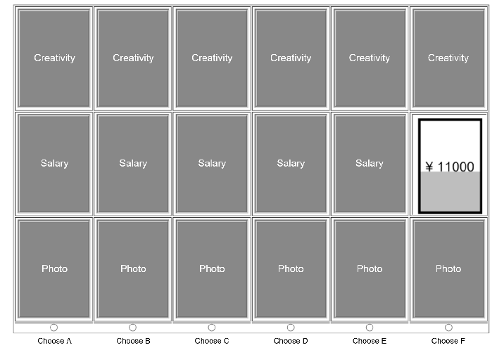
| Figure 3: Example trial of Experiment 2. Each trial contained six different profiles varying on three cues: facial attractiveness, income, and creativity. All information was hidden in the boxes. Participants needed to move the mouse over the box to reveal the information. Once the mouse was moved away from the box, the information was hidden in the box again. Participants could open the boxes as many times as they wanted, until they chose one of the options by clicking the radio button below. The original labels were in Chinese and have been translated into English for illustration purposes. |
At the beginning of each trial, all the information was hidden in boxes with labels displayed on the top of the boxes for participants to locate the information they wanted to acquire. To acquire the information in the boxes, participants had to move the mouse over the boxes to open them. Moving the mouse away from a box would close the box. Participants were allowed to open any box at any time using the mouse.
The experiment consisted of 32 formal trials and three additional filler trials for attention checks. The 32 formal trials were made from the 192 profiles, with each trial containing six profiles. Each filler trial also contained six options. Therefore, the participants were unable to tell whether a trial was a formal or a filler trial before opening the boxes. The fillers, however, had a designated option that the participants were asked to choose. To ensure that participants could find the designated option even if they did not open all the boxes, we added arrows in the neighboring options that navigated the participants to the designated option. The 35 trials were presented in a random order. After the MouseLab task, participants rated the facial attractiveness of all 192 face images using a 7-point scale.
Data pre-processing. In line with previous studies (Payne et al., 1988; Willemsen & Johnson, 2011), we removed box-opening events with acquisition time shorter than 200 ms or longer than 5,000 ms. We excluded three participants who failed more than one attention check trial and two additional participants who on average opened fewer than two boxes per trial. This left us with 3,168 trials from 99 participants for formal data analysis.
Choice models. We used a softmax function to accommodate the one-out-of-six choice structure in the weighted additive choice model and implemented the model under a hierarchical Bayesian framework. In the full choice model WADDFull, the choice probability associated with option ok (ok ∈ {o1,o2, ... ,o6 }) in trial j is defined using the set of predictors as follows:
|
| |
Pr[ok]j= σ
| ⎛
⎝ |
α1 attrjk + α2 incomejk + α3 creatjk + sex · (α4 attrjk + α5 incomejk + α6 creatjk)
| ⎞
⎠ |
|
(3) |
where σ(·) is the softmax function that sets ∑k = 16 Pr[ok]j = 1. Here, attrjk, incomejk and creatjk represent the rated attractiveness, monthly income, and creativity of profile ok for trial j, respectively. Participants may not open some boxes. In such cases, missing values were imputed by the average of the corresponding attribute values across all trials, rather than the hidden values unknown to them (note that the results remain unchanged even if the hidden values were used in the model). sex indicates the participant’s sex, where sex=−0.5 indicates a woman participant and sex=0.5 indicates a man. In the hierarchical Bayesian fit, α1 to α3 were allowed to vary across participants whereas α4 to α6 were held constant across participants, as participant sex was a between-subject factor.
In three additional weighted additive models, we used only one of the three cues for choice predictions. In WADDAttractiveness, we only used the rated attractiveness to predict partner choice and thus turned off α2, α3 ,α5, and α6 in the model. Likewise, WADDIncome, turned off α1, α3 ,α4, and α6, and WADDCreativity turned off α1, α2 ,α4, and α5 in the model.
We fitted the weighted additive choice models using the hierarchical Bayesian method in rstan. The group-level hyperpriors for α1 through α6 were set at the standard normal distribution. For α1 through α3 (the parameters that allowed for individual-level variation), the hyperpriors of individual-level variations (from the group mean) were set using a half-Cauchy distribution (with location = 0 and scale = 5) such that σk ≥ 0. We ran four independent chains, each consisting of 2,500 formal iterations after 1,000 burn-in iterations, totaling 10,000 formal iterations for the posterior approximation. All Rubin-Gelman R were below 1.05, indicating excellent convergence of the MCMC simulation (Gelman & Rubin, 1992).
Markov search model of box-opening data. We used a Markov search model to characterize the value-directed search dynamics in the MouseLab box-opening data on the individual level. The model predicted the switches between the 18 boxes (denoted by S) using transition probabilities Pr[st|st−1], where st−1, st ∈ S and t = 2,3,...,T are the time steps. We further wrote Pr[st|st−1] as a function of the following six sets of predictor variables:
|
| |
Pr[st|st−1]= σ
| ⎛
⎝ |
β1 BtOpt + β2 BtFaceCue + β3 BtCreatCue + β4 ItFaceSameOpt + β5 ItIncomeSameOpt + β6 ItCreatSameOpt +(β7 ItFaceSameOpt + β8 ItIncomeSameOpt + β9 ItCreatSameOpt) · zt−1 + sex · (β10 BtOpt + β11 BtFaceCue + β12 BtCreatCue) + sex · (β13 ItFaceSameOpt + β14 ItIncomeSameOpt + β15 ItCreatSameOpt ) + sex · (β16 ItFaceSameOpt + β17 ItIncomeSameOpt + β18 ItCreatSameOpt)· zt−1
| ⎞
⎠ |
|
(4) |
where σ(·) is the softmax function such that ∑st ∈ SPr[st|st−1] = 1.
In Line 1 of Eq. 4, BtOpt denotes the location of the option associated with st (0 = Leftmost, followed by 0.2, 0.4, 0.6, and 0.8; 1 = Rightmost). BtFaceCue denotes whether st was a face cue or otherwise (1 = Face, 0 = Otherwise). BtCreatCue denotes whether st was a creativity cue or otherwise (1 = Creativity, 0 = Otherwise). We did not include BtIncomeCue in the model to avoid multicollinearity. Therefore, β2 captures the relative search bias of the face cue compared with the income cue and β3 captures the relative search bias of the creativity cue compared with the income cue.
As in Eq. 2, ItFaceSameOpt indicates whether st−1 was a face cue and st and st−1 belonged to the same option (1 = yes, 0 = no). IIncomeSameOpt indicates whether st−1 was an income cue and st and st−1 belonged to the same option (1 = yes, 0 = no). ICreatSameOpt indicates whether st−1 was a creativity cue and st and st−1 belonged to the same option (1 = yes, 0 = no). Therefore β4 through β6 describe the tendencies of within-option search in response to the three types of cues, respectively.
In Line 3, zt−1 stands for the cue value in step st−1. To make the values of different types comparable, we standardized the raw values within each type into z-scores. Therefore, β7 captures the extent to which the observed facial attractiveness determined subsequent within-option switches, β8 captures the extent to which the observed monthly income determined subsequent within-option switches, and β9 captures the extent to which the observed creativity determined subsequent within-option switches.
Lines 4 to 6 captures the sex differences in the various box-opening search tendencies. The three lines correspond to Lines 1–3 respectively. sex indicates whether the participant was a man (sex=0.5) or a woman (sex=−0.5). As sex is a between-participant variable, parameters β10 through β18 in the three lines were held constant across participants (i.e., no individual-level variation was allowed) in the hierarchical Bayesian model fitting.
We also specified starting point probabilities using: Pr[s1|s0] = σ((β1 + β10 · sex)B1Opt + (β2 + β11 · sex)B1FaceCue + (β3 + β12 · sex)B1CreatCue), where s0 represents the start of a trial. This specification allowed the first searched state s1 in each trial to depend on the right-side search bias in β1, the face cue search bias in β2 and the creativity cue search bias in β3, as well as their corresponding sex differences in β10, β11 and β12.
We fitted the Markov search model in rstan using the same settings as in Experiment 1.
Open Practices Statement. We pre-registered Experiment 2 at Open Science Framework (https://osf.io/pzxgd/) after completing the data analysis for Experiment 1. The planned sample size was 50 heterosexual men and 50 heterosexual women. The data and code are available at the same OSF repository.
3.2 Results
Data summary. The proportions of profiles on each of the six locations being chosen ranged from 12.2% to 21.7%. Participants opened an average of 25.4 boxes in each trial to reveal the cue values beneath, meaning that some boxes were opened for more than once. 49.4% of the opened boxes were face cues, 26.5% were income cues, and 24.0% were creativity cues. Face cues attracted much more attention than the other two cues.
The rated attractiveness of female face images was higher than that of the male face images (Mfemale = 3.76, Mmale = 3.38; t382 = 5.86, p < 10−7). However, the standard deviations of the rated attractiveness of female and male face images were comparable (SDfemale = 0.65 versus SDmale = 0.64). Although the average attractiveness differed, the comparable standard deviations of the rated attractiveness of male and female images were important for testing sex differences in the role of facial attractiveness in information search and partner choice.
Cue primacy in choice data. We evaluated to what extent the participants’ choices were determined by the three cues from the hierarchical Bayesian estimation of the full weighted additive choice model (Table 3). On the group level, all three cues positively contributed to the selection of profiles (i.e., α1, α2 and α3 > 0 in Equation 3). There was also a sex difference in the primacy of creativity, whereby creativity played a stronger role in women’s choices than in men’s choices (α6 < 0). The primacy of attractiveness and income appeared not to differ between men and women.
To further determine the relative cue primacy, we evaluated three additional WADD models that used each of the three cues for choice predictions, respectively. Again, we found that the WADDAttractiveness that used simply facial attractiveness as the choice predictor, strongly outperformed the other two choice models, WADDIncome and WADDCreativity, with log Bayes factors (using natural base) of 703 and 812 respectively (Kass & Raftery, 1995). WADDIncome showed stronger predictive performance than WADDCreativity did, with a log Bayes factor (using natural base) margin of 110. Thus, in this experiment, the facial attractiveness is the most important cue for mate preferences, followed by income and creativity, successively.
| Table 3: Hierarchical Bayesian estimation of the full weighted additive choice model in Experiment 2 (Equation 3). |
| 2*Parameter | 2*Interpretation | Posterior estimation |
| | | Mean | 95% CI |
| α1 | Attractiveness | 1.39 | [1.26, 1.52] |
| α2 | Income | 0.98 | [0,82, 1.15] |
| α3 | Creativity | 0.95 | [0.79, 1.10] |
| α4 | Sex × Attractiveness | -0.10 | [-0.34, 0.14] |
| α5 | Sex × Income | -0.14 | [-0.46, 0.18] |
| α6 | Sex × Creativity | -0.34 | [-0.64, -0.03] |
Interactive search dynamics. In the MouseLab box-opening data, we again showed that the value of the acquired information influenced subsequent within-option information acquisition. As Figure 4 shows, attractive faces led to more within-option information acquisitions in the other two cues (i.e., income and creativity) than unattractive faces did. While the within-option transition probability following an unattractive face (i.e., attractiveness rating = 1) was lower than 0.1, the probability of a within-option transition following a highly attractive face (i.e., attractiveness rating = 7) reached as high as 0.4. This pattern was extremely strong for both men and women, as measured by Pearson’s correlation. Similar group-level patterns also emerged for the income and creativity cues among both men and women.
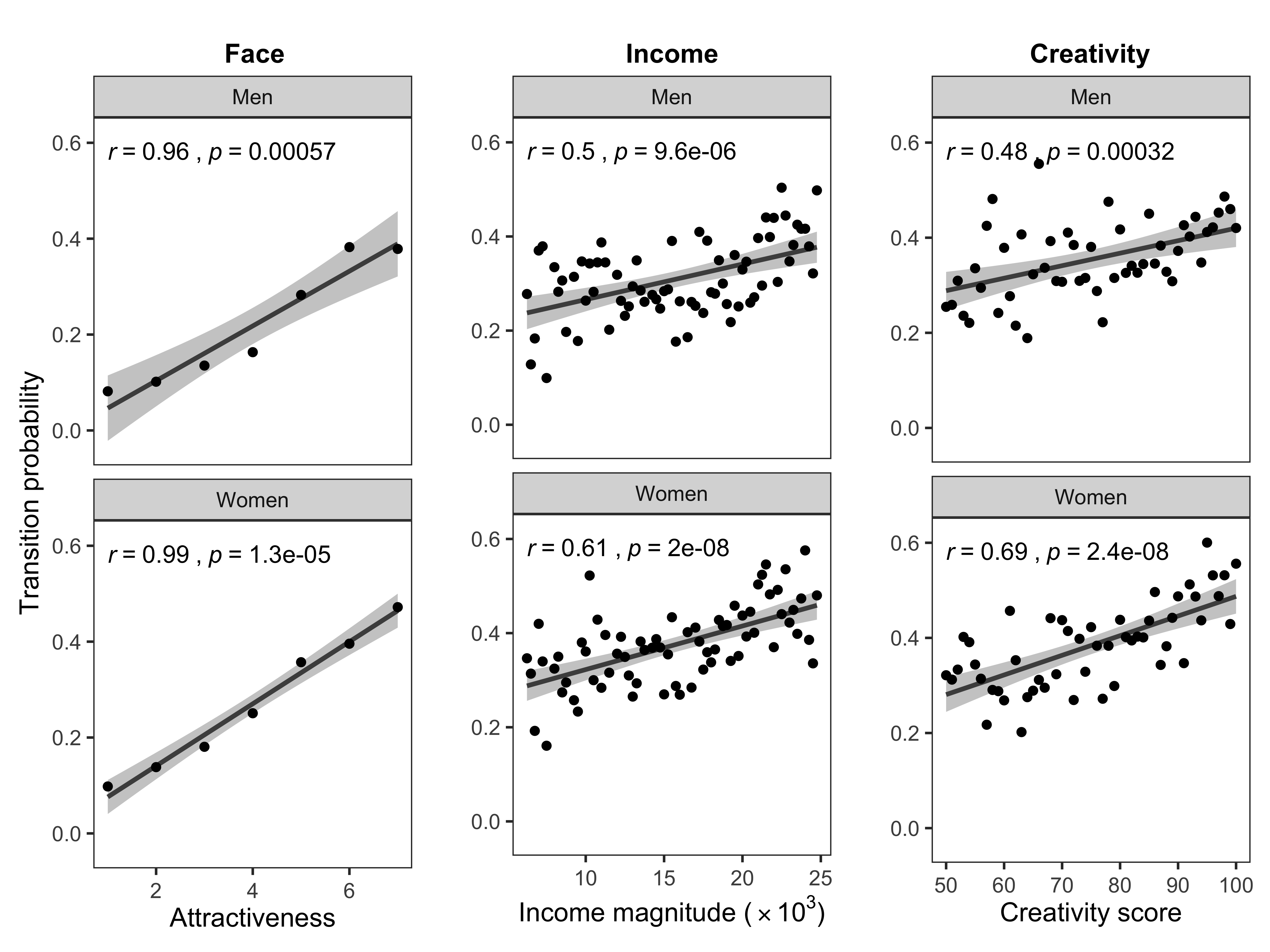
| Figure 4: Interactive search dynamics in Experiment 2. Group-level correlations between cue desirability and subsequent within-profile transition probabilities, separately for men and women. |
We characterized these patterns more rigorously using a Markov search model, fitted to the information acquisition data under a hierarchical Bayesian framework (see Table 4 for a summary of group-level parameters). On the group level, the model suggested that value-directed interactive search was strong for all three cues (β7, β8, β9 > 0), and that the strength of interactive search was stronger for the face cues than the income cues (β7 − β8 = 0.22, 95% CI = [0.15, 0.30]) and the creativity cues (β7 − β9 = 0.24, 95% CI = [0.18, 0.31]). The extent of interactive search in response to income did not differ from that in response to the creativity cue (β8 − β9 = 0.02, 95% CI = [-0.05, 0.09]). Additionally, the participants exhibited substantial left-side search bias (β1 < 0). They searched more often for facial information (β2 > 0), but less creativity information (β3 < 0) than searching for the income information. They were also likely to make within-option transition in response to all types of cues (β4, β5, β6 > 0).
The Markov search model also allowed us to examine the sex differences in the various search dynamics. There was slight evidence suggesting that men made more attractiveness-directed interactive search than women did (β16>0), while the former’s income- and creativity-directed interactive search were slightly weaker than the latter’s (β17, β18< 0, though their 95% CIs include 0). Other sex differences included men exhibited more left-side search bias (β10<0) and fewer within-option transitions (β13,β14,β15 <0) than women did.
| Table 4: Hierarchical Bayesian estimation of the Markov search model in Experiment 2 (Equation 4). |
| 2*Parameter | 2*Interpretation | Posterior estimation |
|
| | Mean | 95% CI |
| β1 | Right bias | -0.19 | [-0.22, -0.16] |
| β2 | Face bias | 0.68 | [0.55, 0.80] |
| β3 | Creativity bias | -0.11 | [-0.22, -0.01] |
| β4 | FaceSameOption | 0.25 | [0.11, 0.38] |
| β5 | IncomeSameOption | 1.21 | [1.06, 1.35] |
| β6 | CreativitySameOption | 1.10 | [0.96, 1.24] |
| β7 | FaceSameOption×Attractiveness | 0.44 | [0.40, 0.49] |
| β8 | IncomeSameOption×Magnitude | 0.22 | [0.16, 0.27] |
| β9 | CreativitySameOption×Score | 0.20 | [0.15, 0.24] |
| β10 | Sex×Right | -0.08 | [-0.15, -0.02] |
| β11 | Sex×Face | -0.05 | [-0.30, 0.20] |
| β12 | Sex×Creativity | -0.02 | [-0.21, 0.18] |
| β13 | Sex×FaceSameOption | -0.29 | [-0.58, -0.01] |
| β14 | Sex×IncomeSameOption | -0.22 | [-0.52, 0.06] |
| β15 | Sex×CreativitySameOption | -0.30 | [-0.58, -0.01] |
| β16 | Sex×FaceSameOption×Attractiveness | 0.09 | [-0.01, 0.18] |
| β17 | Sex×IncomeSameOption×Magnitude | -0.08 | [-0.19, 0.03] |
| β18 | Sex×CreativitySameOption×Score | -0.04 | [-0.13, 0.05] |
3.3 Discussion
The MouseLab data in Experiment 2 replicated and extended the findings in the eye-tracking study in Experiment 1. The interactive search dynamics were strong for all three cues, including the newly added creativity. We once again showed that the extent of interactive search dynamics depends on cue primacy. The interactive search dynamics were particularly strong in response to faces, followed by those in response to the income and creativity cues. We also observed some evidence on the interaction between cue type and participant sex on the magnitude of interactive search dynamics, as predicted. This interaction is consistent with the differential cue primacy among men and women.
4 Compensatory versus non-compensatory choice strategies
As a distinct feature of our paper, we primarily focus on the information search strategies during partner selection in the above sections. Yet in the extant literature, the heuristics or smart shortcuts people rely on for partner selection are typically framed as decision strategies that immediately lead to final choices. To make a closer connection to this strand of literature (Brandner et al., 2020; Conroy-Beam, 2018; Lenton et al., 2013; Miller & Todd, 1998), we revisit the ideas of compensatory versus non-compensatory choice strategies that are directly fitted to the choice data. To this end, we formulate instances of compensatory and non-compensatory choice models respectively, and compared their relative accuracy in describing the choice data.
4.1 Aspiration model
We compared the full weighted additive model with the aspiration choice model (Miller & Todd, 1998), as an instance of non-compensatory models. Since we have distinguished the evaluation process from the information search process, following Brandner et al. (2020), we treated the aspiration model as an atemporal choice model (i.e., the model assumes simultaneous evaluation of all the cues). Therefore, the aspiration model assumes that the decision maker compares each cue value with some threshold (i.e.,the aspiration level) and then accumulates the support for an option depending on whether its cue values exceed the corresponding thresholds. In the experiment, the activation of ojk, the kth option in trial j is defined as:
|
ajk = | |
| ⎧
⎨
⎩ | | cjkl ≥ tl 0cjkl < tl |
|
(5) |
where L=2 (in Experiment 1) or 3 (in Experiment 2) represents the number of cues, tl is a free parameter that represents the decision maker’s threshold for cue l, and cjkl is the cue value in option ojk. For undisclosed cue value cjkl in Experiment 2, we replaced cjkl with the mean attribute value. For each trial j, the values of ajk were passed to the softmax function (or its reduced form, logistic function, in Experiment 1) to generate the probability of choosing ojk.
Because of the discontinuous nature of the aspiration model (i.e., the likelihood function is not a continuous function of free parameters), the hierarchical Bayesian fitting method using Hamilton Markov chain in rstan was inappropriate. We thus used the maximum likelihood method to evaluate the models’ goodness of fit to data at the individual level and penalized model complexity using Akaike information criterion (AIC). The lower the AIC value, the better the model performance.
4.2 Experiment 1 results
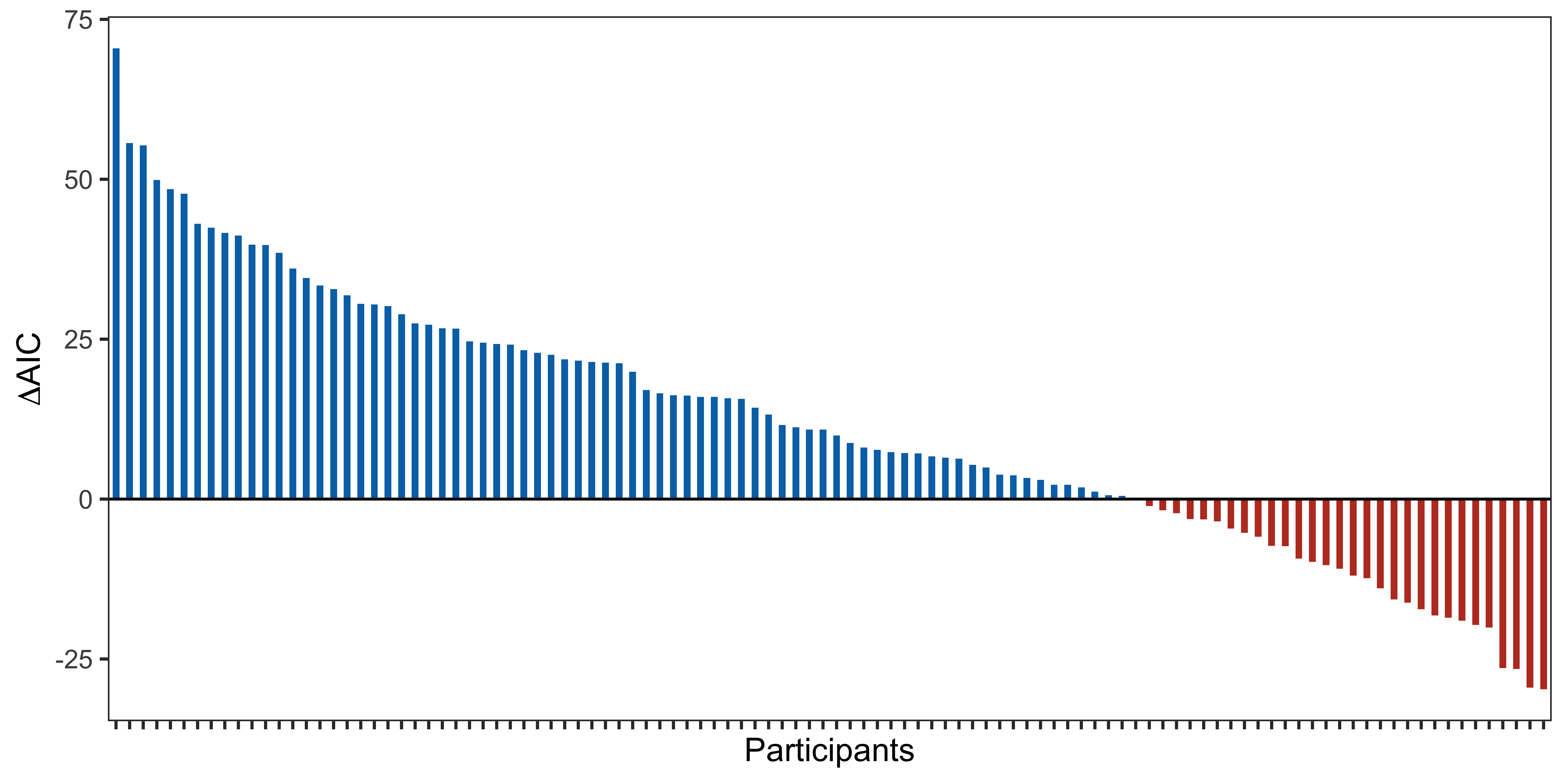
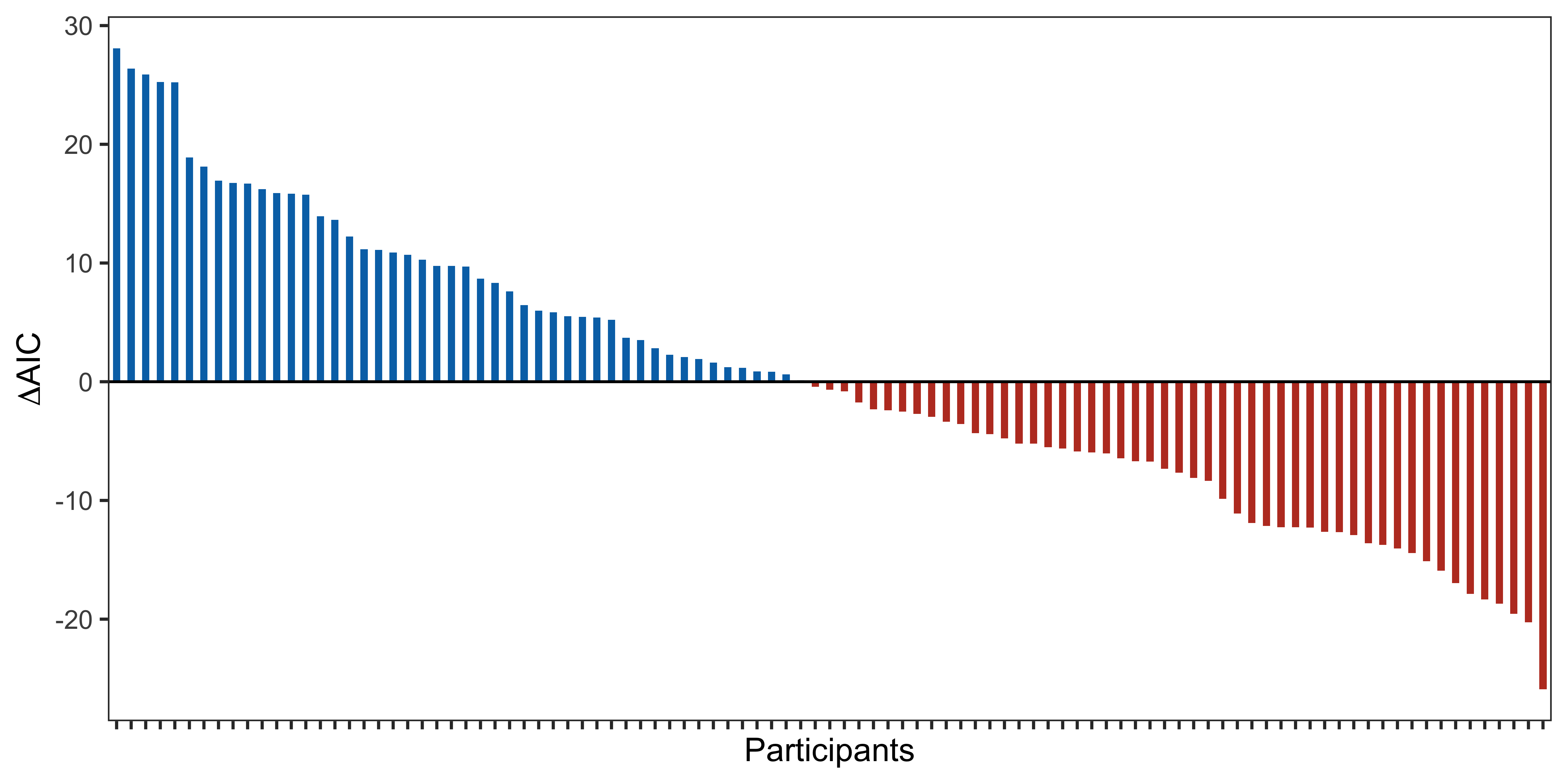
In Experiment 1, we found that the aggregate AIC across participants of the full weighted additive model was much lower than that of the aspiration model (AICWADD = 11257; AICAspiration = 12491), indicating that the weighted additive model fitted the choice data better than the aspiration model. Individually, 72% of the participants were better fitted by WADD, according to AIC, while only 28% were better fit by the aspiration model (Figure 5). These results were consistent with previous findings using two-alternative choice experiments (Brandner et al., 2020; Conroy-Beam, 2018).
| Figure 5: Individual-level model comparison between the weighted additive model and the aspiration model in Experiment 1. Positive AIC differences (blue bars) indicate the participants were better fitted by the weighted additive model while negative AIC differences (red bars) indicate the participants were better fitted by the aspiration model (N = 106). |
4.3 Experiment 2 results
In Experiment 2, we found that the aggregate AIC across participants of the full weighted additive model was slightly lower than that of the aspiration model (AICWADD = 6610; AICAspiration = 6630). Individually, 48% of the participants were better fit by WADD, according to AIC, and the remaining 52% were better fit by the aspiration model (Figure 6). Overall, the two choice models described the choice data almost equally well in Experiment 2.
| Figure 6: Individual-level model comparison between the weighted additive model and the aspiration model in Experiment 2. Positive AIC differences (blue bars) indicate the participants were better fitted by the weighted additive model while negative AIC differences (red bars) indicate the participants were better fitted by the aspiration model (N = 99). |
4.4 Discussion
Our model comparison results are largely consistent with existing literature using similar methods. In most cases, the compensatory choice strategies describe the choice data better than non-compensatory choice strategies, especially when there are only two options in each choice. However, we also observed that the descriptive gap between the WADD and the aspiration models became minimal in Experiment 2. Two possible reasons may underlie this difference between Experiments 1 and 2. One was that Experiment 2 involved more cues and more options than Experiment 1 did. The other was that the MouseLab paradigm revealed only one piece of information at a time. Both factors made it more cognitively demanding for the participants to hold all numeric information in memory as required by the weighted additive models. Nevertheless, our hypothesized interactive search dynamics was robust enough, regardless of the number of cues and options involved in each decision.
5 General discussion
Seeking the right person to date and to live with is a decision of considerable significance. Mainstream theories of partner selection suggest that people search for and choose romantic partners efficiently using heuristics, relying on incomplete information. However, extant experimental work rarely finds evidence for heuristic rules in partner choices but rather suggests that humans’ mate choices are consistent with compensatory choice strategies that take all relevant information into consideration.
Our research resolves this conflict by disentangling the information acquisition process from the evaluation process in the partner choice problem. In light of the latest insights from cognitive science studies, efficient information acquisition for rational choice requires smart heuristic search strategies (Callaway et al., 2021; Jang et al., 2021). In two process-tracing experiments, we found that the information acquisition process for partner choice displayed interactive search dynamics that corresponded to the heuristic rules proclaimed in the literature (Lenton et al., 2013; Miller & Todd, 1998): High cue values increase subsequent information acquisition within profiles, and low cue values decrease subsequent information acquisition within profiles. We extended our test by examining how such interactive search dynamics varied across cue types and participant sexes, depending on cue primacy.
The value-directed search can be also interpreted as an alternative implementation of the sequential aspiration mate search strategy (Miller & Todd, 1998), focusing primarily on information gathering between different cues that signal a potential candidate’s mate value. Our study provides novel experimental evidence in support of the prominent theories of mate search. We did so by distinguishing the information search process from the evaluation process in mate choice. Further analysis of the choice data suggests that such value-directed search heuristics do not necessarily lead to non-compensatory choices, at least when the choice involves a relatively small number of potential candidates.
The value-directed search dynamics for partner choice are consistent with similar evidence emerging in related domains of value-based decision-making (Glöckner & Betsch, 2008; Holyoak & Simon, 1999; Jekel et al., 2018; Scharf et al., 2019). The term “attraction” is used in search heuristics, where “attraction” refers to the overall attractiveness of an option. For example, in a risky choice, the decision-maker’s information search for payoffs depends on their associated probabilities (Fiedler & Glöckner, 2012). This pattern appears to support the idea that human decision-making is susceptible to biases due to cognitive limitations (Kahneman et al., 1982) and a complex decision environment (Gigerenzer & Todd, 1999; Payne et al., 1988). However, recent cognitive science research suggests that such value-directed searches may serve optimal evidence accumulation according to a normative decision rule (e.g., expected utility theory) (Callaway et al., 2021; Li & Ma, 2021).
While “attraction” search suggests that the overall attractiveness of an option leads to more attention to the option, our model assumes that a high-value cue signals the option’s potentially high overall attractiveness, which in turn increases within-option search. Despite this implementation difference, our value-directed search and the “attraction” search are built upon the same idea that the (potentially) high value of an option increases the decision maker’s interest in and attention to it. Cue values serve as the proxies of the overall mate value in an option. Consistently, we found that the extent of interactive search was stronger in response to high-primacy cues (which was more indicative of overall attractiveness) than for low-primacy cues.
How do people integrate cue values into a mate value in the face of incomplete information? In this paper, we imputed the missing values with attribute means and specified two choice strategies. Overall, the compensatory weighted additive model described the choice data better than non-compensatory aspiration model. However, the comparison between Experiments 1 and 2 suggests that the rule that governs the integration of different cues may change depending on task properties and its cognitive demand. When the decision was loaded with many options and cues, aggregation strategies that required less numeric information may play an increased role. Decision strategies are the focus of judgment and decision making research at large. There exist various theoretical perspectives. For example, the sequential evidence accumulation framework suggests that the decision maker keeps accumulating evidence for each option under consideration based on the mere recording of the attended information, and a decision is reached when the amount of the accumulated evidence hits a preset boundary (Bhatia, 2013; Krajbich & Rangel, 2011; Roe et al., 2001). Yet the inferential approach suggests that the decision maker may carry out cognitive imputing that facilitates compensatory evaluation of candidates (Callaway et al., 2021; Li & Ma, 2021). When dealing with unsearched information, decision makers may be able to reconstruct its value from their general knowledge of the situation (Elwin et al., 2007). The decision strategies in partner choice may also be related to strategies in other types of decision making, and thus can be informed by the latter. Hence, there is room for further investigation into how people integrate cue values into a mate choice response, especially when confronting a relatively large number of candidates.
Finally, real-world partner choice is more complex than in our experiments. One may encounter many more potential partners varying on many more dimensions. Furthermore, in the real world, the acquired information is noisy because of factors such as the incentive to deceive about one’s suitability and secondhand information. It remains unclear how value-direct search responds to the (in)credibility of information. Prior work has suggested that such selection biases in information seeking explain a number of phenomena in behavioral and social sciences (Denrell, 2005; Le Mens & Denrell, 2011). We look forward to future work that unpacks the cognitive basis of mate search and choice in this direction.
References
Arbuthnott, D., Fedina, T. Y., Pletcher, S. D., & Promislow, D. E. (2017). Mate choice in fruit flies is rational and adaptive. Nature Communications, 8(1), 1–9.
Bhatia, S. (2013). Associations and the accumulation of preference. Psychological Review, 120(3), 522–543.
Brandner, J. L., Brase, G. L., & Huxman, S. A. (2020). “Weighting” to find the right person: Compensatory trait integrating versus alternative models to assess mate value. Evolution and Human Behavior, 41(4), 284–292.
Buss, D. M. (1989). Sex differences in human mate preferences: Evolutionary hypotheses tested in 37 cultures. Behavioral and Brain Sciences, 12(1), 1–14.
Buss, D. M., & Barnes, M. (1986). Preferences in human mate selection. Journal of Personality and Social Psychology, 50(3), 559–570.
Buss, D. M., & Schmitt, D. P. (1993). Sexual strategies theory: An evolutionary perspective on human mating. Psychological Review, 100(2), 204–232.
Buss, D. M., Shackelford, T. K., Kirkpatrick, L. A., & Larsen, R. J. (2001). A half century of mate preferences: The cultural evolution of values. Journal of Marriage and Family, 63(2), 491–503.
Callaway, F., Rangel, A., & Griffiths, T. L. (2021). Fixation patterns in simple choice reflect optimal information sampling. PLoS Computational Biology, 17(3), Article e1008863.
Chiappori, P. A. (2020). The theory and empirics of the marriage market. Annual Review of Economics, 12, 547–578.
Conroy-Beam, D. (2018). Euclidean mate value and power of choice on the mating market. Personality and Social Psychology Bulletin, 44(2), 252–264.
Dechaume-Moncharmont, F.-X., Freychet, M., Motreuil, S., & Cézilly, F. (2013). Female mate choice in convict cichlids is transitive and consistent with a self-referent directional preference. Frontiers in Zoology, 10(1),
1–10.
Denrell, J. (2005). Why most people disapprove of me: Experience sampling in impression formation. Psychological Review, 112(4), 951–978.
Dupuy, A., & Galichon, A. (2014). Personality traits and the marriage market. Journal of Political Economy, 122(6), 1271–1319.
Eagly, A. H., & Wood, W. (1999). The origins of sex differences in human behavior: Evolved dispositions versus social roles. American Psychologist, 54(6), 408–423.
Elwin, E., Juslin, P., Olsson, H., & Enkvist, T. (2007). Constructivist coding: Learning from selective feedback. Psychological Science, 18(2), 105–110.
Fiedler, S., & Glöckner, A. (2012). The dynamics of decision making in risky choice: An eye-tracking analysis. Frontiers in Psychology, 3, 335.
Gale, D., & Shapley, L. S. (1962). College admissions and the stability of marriage. The American Mathematical Monthly, 69(1), 9–15.
Gelman, A., & Rubin, D. B. (1992). Inference from iterative simulation using multiple sequences. Statistical Science, 7(4), 457–472.
Gigerenzer, G., & Goldstein, D. G. (1996). Reasoning the fast and frugal way: Models of bounded rationality. Psychological Review, 103(4), 650–669.
Gigerenzer, G., & Todd, P. M. (1999). Fast and frugal heuristics: The adaptive toolbox. In G. Gigerenzer, P. Todd, & the ABC Research Group (Eds.), Simple heuristics that make us smart (pp. 3–34). Oxford University Press.
Glöckner, A., & Betsch, T. (2008). Modeling option and strategy choices with connectionist networks: Towards an integrative model of automatic and deliberate decision making. Judgment and Decision Making, 3(3), 215–228.
Gluth, S., Kern, N., Kortmann, M., & Vitali, C. L. (2020). Value-based attention but not divisive normalization influences decisions with multiple alternatives. Nature Human Behaviour, 4(6), 634–645.
Goodrich, B., Gabry, J., Ali, I., & Brilleman, S. (2020). rstanarm: Bayesian applied regression modeling via Stan. https://mc-stan.org/rstanarm.
Holyoak, K. J., & Simon, D. (1999). Bidirectional reasoning in decision making by constraint satisfaction. Journal of Experimental Psychology: General, 128(1), 3–31.
Jang, A. I., Sharma, R., & Drugowitsch, J. (2021). Optimal policy for attention-modulated decisions explains human fixation behavior. Elife, 10, Article e63436.
Jekel, M., Glöckner, A., & Bröder, A. (2018). A new and unique prediction for cue-search in a parallel-constraint satisfaction network model: The attraction search effect. Psychological Review, 125(5), 744–768.
Kahneman, D., Slovic, P., & Tversky, A. (1982). Judgment under uncertainty: Heuristics and biases. Cambridge University Press.
Kass, R. E., & Raftery, A. E. (1995). Bayes factors. Journal of the American Statistical Association, 90(430), 773–795.
Kenrick, D. T., Groth, G. E., Trost, M. R., & Sadalla, E. K. (1993). Integrating evolutionary and social exchange perspectives on relationships: Effects of gender, self-appraisal, and involvement level on mate selection criteria. Journal of Personality and Social Psychology, 64, 951–969.
Krajbich, I., & Rangel, A. (2011). Multialternative drift-diffusion model predicts the relationship between visual fixations and choice in value-based decisions. Proceedings of the National Academy of Sciences, 108(33), 13852–13857.
Le Mens, G., & Denrell, J. (2011). Rational learning and information sampling: On the "naivety" assumption in sampling explanations of judgment biases. Psychological Review, 118(2), 379–392.
Lenton, A. P., Penke, L., Todd, P. M., & Fasolo, B. (2013). The heart has its reasons: Social rationality in mate choice. In R. Hertwig, U. Hoffrage, & the ABC Research Group (Eds.), Simple heuristics in a social world (pp. 433–457). Oxford University Press.
Li, Z.-W., & Ma, W. J. (2021). An uncertainty-based model of the effects of fixation on choice. PLoS Computational Biology, 17(8), Article e1009190.
Miller, G. F., & Todd, P. M. (1998). Mate choice turns cognitive. Trends in Cognitive Sciences, 2(5), 190–198.
Payne, J. W., Bettman, J. R., & Johnson, E. J. (1988). Adaptive strategy selection in decision making. Journal of Experimental Psychology: Learning, Memory, and Cognition, 14(3), 534–552.
Payne, J. W., Bettman, J. R., & Johnson, E. J. (1993). The adaptive decision maker. Cambridge University Press.
Roe, R. M., Busemeyer, J. R., & Townsend, J. T. (2001). Multialternative decision field theory: A dynamic connectionst model of decision making. Psychological Review, 108(2), 370–392.
Scharf, S. E., Wiegelmann, M., & Bröder, A. (2019). Information search in everyday decisions: The generalizability of the attraction search effect. Judgment and Decision Making, 14(4), 488–512.
Sepulveda, P., Usher, M., Davies, N., Benson, A. A., Ortoleva, P., & De Martino, B. (2020). Visual attention modulates the integration of goal-relevant evidence and not value. Elife, 9, Article e60705.
Stan Development Team. (2021). RStan: the R interface to Stan. R package version 2.21.3. https://mc-stan.org/
Wang, H., He, Z., & He, L. (2021). Transitive mate preferences. Decision, 8(3), 180–201.
Willemsen, M. C., & Johnson, E. J. (2011). Visiting the decision factory: Observing cognition with MouselabWEB and other information acquisition methods. In M. Schulte-Mecklenbeck, A. Köhberger, & J. Johnson (Eds.), A handbook of process tracing methods for decision research (pp. 21–42). Psychology Press.
This document was translated from LATEX by
HEVEA.