Judgment and Decision Making, Vol. ‍17, No. ‍5, September 2022, pp. 1015-1042

Abstract: Loss aversion, the argument that losses are given more weight than gains, has been recently shown to be absent in small losses. However, a series of studies by Mrkva et al. (2020) appear to demonstrate the existence of loss aversion even for smaller losses. We re-ran Mrkva et al.’s decision tasks after removing features of the task that differentiated losses from the gains, particularly asymmetries in sizes of gains and losses, an increasing order of losses, and status quo effects. The results show that we replicate Mrkva et al.’s (2020) findings in their original paradigm with online participants, yet in five studies where gains and losses were symmetrically presented in random order (n = 2,001), we find no loss aversion for small amounts, with loss aversion surfacing very weakly only for average losses of $40 (mean λ = 1.16). We do find loss aversion for higher amounts such as $100 (mean λ = 1.54) though it is not as extreme as previously reported. Furthermore, we find weak correlation between the endowment effect and loss aversion, with the former effect existing simultaneously with no loss aversion. Thus, when items are presented symmetrically, significant loss aversion emerges only for large losses, suggesting that it cannot be argued that (all) “losses loom larger than gains.”

Keywords: loss aversion, incentive size, endowment effect, biases

1 Introduction

“Dulce periculum” (danger is sweet)

Horace, Odes III, 25, 16

Loss aversion, the notion that losses are given more subjective weight than gains (Kahneman & Tversky, 1979), is considered one of the most important contributions of psychology to the emerging science of behavioral economics (Kahneman, 2011). However, the existence and magnitude of loss aversion is also one the most debated issues in behavioral economics today (see e.g., Gal & Rucker, 2018; Yechiam, 2019; Mrkva, Johnson, Gachter & Herrmann, 2020). The current study aims to revisit a recent set of findings showing that loss aversion can be demonstrated even in small monetary amounts (Mrkva et al., 2020). We argue that this and similar studies may have been using research methods that bias towards loss aversion and produce conflating evidence.

The polarity of the issue can perhaps best be illustrated by the results of two (yet unpublished but already influential) meta-analyses. Both used the extant literature on loss aversion to estimate the value of λ (loss aversion parameter) which dictates how much a loss outcome is given more subjective weight than a respective gain outcome.¹ The first meta-analysis is by Walasek, Mullett and Stewart (2018). In their analysis the mean λ across studies was 1.31, with a lower confidence interval of 1.1 which is rather close to 1 (implying gain-loss neutrality) and a far cry from the initial postulation by Tversky and Kahneman (1992) that losses have more than twice the weight of gains (i.e., λ = 2.25). Additionally, only six out of 19 studies in this meta-analysis observed significant loss aversion. These findings challenge the claim that loss aversion is reliable and robust. On the other hand, a meta-analysis by Brown, Imai, Vieider and Camerer (2021) examined a much broader literature and used more lenient inclusion criteria. Its results indicate a confidence interval between 1.8 and 2.1 for λ. These starkly different findings seem to be due to the examination of different literatures, different types of tasks used to elicit loss aversion, and different versions of the models used to estimate λ (i.e., prospect theory). Importantly, the gap also emphasizes the fact that there’s no done deal in this story, and suggests the importance of revisiting prior findings in a meticulous fashion.

A key issue in the debate on loss aversion is whether it is revealed only for large losses, or also for small losses. The existence of loss aversion in smaller losses is important both empirically and theoretically. Theoretically, loss aversion is differentiated from the previous notion of risk aversion (e.g., Markowitz, 1952; Pratt, 1964; Sharpe, 1964) in arguing for a simple linear subjective weighting of losses to gains which is not a function of the size of the outcome (or in other words, that even small symmetrical risks-benefits are avoided). Moreover, it has been formally demonstrated by Hansson (1988) and Rabin (2000) that if people are loss averse for small amounts, this implies that under expected utility theory with a concave utility function, they should show puzzlingly high risk-aversion rates.² Thus, the emergence of loss aversion for smaller losses results in baffling predictions for a simple expected utility model.

Yet inconsistently with the notion that loss aversion emerges for smaller losses, a recent string of studies showed that for small losses individuals do not reliably show loss aversion, but rather exhibit loss-gain neutrality (Ert & Erev, 2013; Yechiam & Hochman, 2013; Gal & Rucker, 2018; Yechiam, 2019) and even gain seeking in some settings (Gal & Rucker, 2018).

Reacting to these findings, Mrkva et al. (2020) argued that loss aversion is “alive and well” even for small outcomes. They examined two behavioral phenomena which they argue are demonstrative of loss aversion. The first is avoiding risky outcomes involving losses. Specifically, participants were asked if they agree to accept (i.e., take) or reject a series of lotteries and investments, with increasing losses. For instance, in their “lottery task” the first lottery involved a coin toss for either losing 2 Euros or winning 6 Euros, the second lottery had a larger loss of 3 Euros, etc., up to 7 Euros. The second phenomenon is the endowment effect, the tendency to valuate sold objects more than purchased ones (Thaler, 1980). While this phenomenon may be driven by other factors besides loss aversion (as noted in Gal, 2006; Morewedge & Giblin, 2015; and see also Plott & Zeiler, 2005), Mrkva et al. (2020) suggested that a correlation between the size of the endowment effect and the estimated loss aversion for risky lotteries implies that both are related to the same construct.

Mrkva et al.’s (2020) results using a very large sample showed a mean λ parameter higher than 1 (indicatory of loss aversion) in all of their studies of risky lotteries and investments, even for small losses of 2 to 7 Euros. Moreover, in most of their studies the mean λ topped the 2.25 observed in the seminal study by Tversky and Kahneman (1992). There was also a strong correlation between λ in hypothetical investments and the extent of the endowment effect calculated for the same participants.

However, there are important details that must be considered when evaluating these results, and those of previous studies that used the same approach for extracting the loss aversion parameter (e.g., Tversky & Kahneman, 1992; Shang et al., 2021), which could be referred to as the “list method” (Holt & Laury, 2002) and is indeed one of the most popular ways of quantifying loss aversion in the literature (see e.g., Brown et al., 2021).

The first and perhaps most important feature of the list method is that gains and losses are asymmetric, and therefore random noise and ranking-based choices may bias participants towards loss aversion (as also noted by Mrkva et al., 2020; and see related results in Ert & Erev, 2013; Walasek & Stewart, 2019; Rakow, Cheung & Restelli, 2020). For example, in Study 1B, Mrkva et al. (2020) examined the response to investments with a 50:50 chance of winning $100 and losing either $10, $25, $50, or $100 (in different investments). Notice the asymmetry of gains and losses. Under prospect theory (specified with a linear value/utility function, as detailed in Study 1), responding “reject” to all four items implies a lower boundary of 10 for λ, while rejecting three to zero items (in order) implies a lower boundary of 4, 2, 1.33, and 0, respectively. Therefore, if a person answers randomly s/he would have a mean orthodox λ of 3.47, and random error biases responses in the direction of loss aversion (see also Budescu, Wallsten & Au, 1997). In addition, if a person is highly sensitive to the ranking of gains and losses, they would similarly opt for the option with the middle-sized loss producing an inflated λ score (Walasek & Stewart, 2019).

Secondly, because losses presented in the list method steadily increase some participants may treat multiple items inter-relatedly and accept the lottery with the lowest loss, as if it was the “most correct” answer in a multiple-choice exam. Thus, the monotonically increasing size of losses may further bias participants towards loss aversion. Thirdly, the list method typically conflates loss aversion with the status quo effect because rejecting the lottery (and avoiding losses) is the status quo (Ert & Erev, 2013; Yechiam & Hochman, 2013).³ Notice that these effects not only potentially increase loss aversion but can also create a false correlation between the endowment effect and loss aversion. This correlation could result from the similarity of the phrasing and the fact that participants who treat the task as a multiple-choice test would aim to get the best “bargain” in both.⁴

Here, we aimed to examine whether these features of the list method provide sufficient conditions for the gap between Mrkva et al.’s (2020) results and the absence of loss aversion recorded in other studies (e.g., Ert & Erev, 2013; Gal & Rucker, 2018). Our study can be thought of as extending the critique of Ert and Erev (2013) on the list method with the additional novel prediction that the monotonic order of outcomes sizes inflates loss aversion, in addition to the non-symmetry of gains and losses and the status quo effect (examined by Ert and Erev, 2013). Indeed, Ert and Erev (2013) were not able to significantly replicate loss aversion in their study of the “original” list method, and this may be because they used a random rather than increasing-losses order. By examining all three features of the list method – asymmetry of items, order, and status quo – we wish to shed light and explicate the gap between the arguments made in favor and against loss aversion, and specifically the argument that loss aversion emerges both for smaller and larger losses, versus the counter-claim that it only emerges for larger losses.

Following Kahneman and Tversky’s (1979) original postulation that loss aversion implies that “most people find symmetric bets of the form (x, .50; -x, .50) distinctly unattractive” (p. 279), and the modeling critique of Walasek et al. (2018), our primary dependent variable is a behavioral measure of loss aversion given symmetric gains and losses. In addition, we also approximated λ, using the exact same modeling approach as in Mrkva et al. (2020). In the first five studies we focused on the emergence of loss aversion in decisions under risk and experimentally tested the possible effect of items order (increasing versus random losses), the status quo bias, the size of the outcomes, and task instructions (lottery versus investment task). In the last study we examined the possible correlation between loss aversion and the endowment effect.

2 Study 1: Replication and the effect of random order

Our studies were administered online with Prolific Academic participants. Therefore, given the different population from that of Mrkva et al. (2020) it was important for us to try and replicate their results using their original lottery and investment tasks. In addition, in this study we examined the effect of the increasing losses used in Mrkva et al. (2020). As noted above, we argue that these monotonic increases can lead to a mindset that different items are inter-related. This can escalate loss aversion because some participants may treat items interconnectedly and select the “best answer” of partaking the lottery (or investment) with the smallest loss. We therefore compared an increasing-loss order to a condition where items are randomly ordered.

2.1 Method

2.1.1 Participants

All studies were conducted with Prolific Academic workers from the USA, UK, Ireland, Australia, and Canada who had an approval rate of at least 95% and who stated that English was their first language. Higher approval rates on Prolific are associated with less dishonest behavior (Schild, Lilleholt & Zettler, 2019). A total of 400 participants (199 females, 197 males, 4 other) volunteered to take part in the study.⁵ Their average age was 37.4 (SD = 12.7) with individuals ranging from 18 to 78 years old. From this sample, 201 participants were randomly allocated to the increasing-loss condition and 199 participants were allocated to the random-loss condition. Participants provided informed consent statements, and all studies were ethically approved by the authors’ university ethics committee. Participants in both conditions received a fee of $1 for completing the study.

2.1.2 Task

We administered Mrkva et al.’s (2020) lottery task (from their Study 1) followed by the investment task (from their studies 2B-2D). The increasing-loss condition conformed to the exact order of items as in Mrkva et al, with the first items having the smallest losses, and with the loss monotonically increasing from item to item (see supplementary section for the exact items and their order). In the random-loss version we used the exact same items, but their order was separately randomized for each participant. Subsequent studies also controlled for task order (lottery vs. investment). Complete task instructions are presented in Appendix A. Each item (lottery/investment) was presented on a separate screen with a “next” button to move to the next item. In total, the two tasks included 10 items. Following these two tasks, participants completed a short demographic questionnaire in which they reported their age, gender, education, and definition of wealth and household income (following Mrkva et al., 2020; see supplementary section).

2.1.3 Analysis

We used two indicators of loss aversion: First, we examined risk taking for the lottery with symmetric gains and losses (following Kahneman & Tversky, 1979). Secondly, the loss aversion coefficient λ was cautiously estimated for each individual participant by dividing the constant gain (e.g., 6 in the lottery task, 100 in the investment task) by the smallest loss for which the gamble was not accepted (see also Hermann, 2017), as in Mrkva et al. (2020). Mrkva et al.’s (2020) basic version of prospect theory assumed a linear weighting function, namely no diminishing sensitivity (indeed for the amount sizes used here, no strong diminishing sensitivity is expected; Abdellaoui, Bleichrodt & L’Haridon, 2008). It also assumes no probability weighting. This latter assumption is not material because given that the probabilities are the same for gains and losses in all of the lotteries we used, the multiplication of the probability weight is canceled out because it is identical for the gain and loss components (and immaterial for the zero outcome).

For example, respondents who accepted the investment producing $100 gain and $25 loss with 50%, but not the respective investment with $100 gain and $50 loss were coded as having a λ of 2 because their value function (V) gives more weight to the loss component V(−|50^α|) than the gain component of the lottery V(100^α)), and assuming α to be 1, the minimal λ required to reject the lottery is 2. Importantly, we also used a version of prospect theory with diminishing sensitivity based on previously estimated values of α , and this is reported in the supplementary section.

As in Mrkva et al. (2020), we excluded participants who provided nonmonotonic responses from this modeling analysis. All effects remained similar in size when using alternative modeling approaches (see supplementary section). Throughout, we report both the median and average λ because each has relative faults and advantages. The median does not take into account the precise value of each observation and may be particularly biased when there is a large disparity between responses. This is likely given low-grain items with respect to the size of gains and losses.⁶ On the other hand, the average loss aversion is biased. For example, consider an individual who gives losses twice the weight of gains. Her λ would be 2. Now consider the “opposite” character who gives gains twice the weight of losses. Her λ would be 0.5. On average, their λ would be 1.25 although clearly the non-biased central tendency should be loss neutrality (i.e., λ = 1); the latter is represented by the median.

2.2 Results

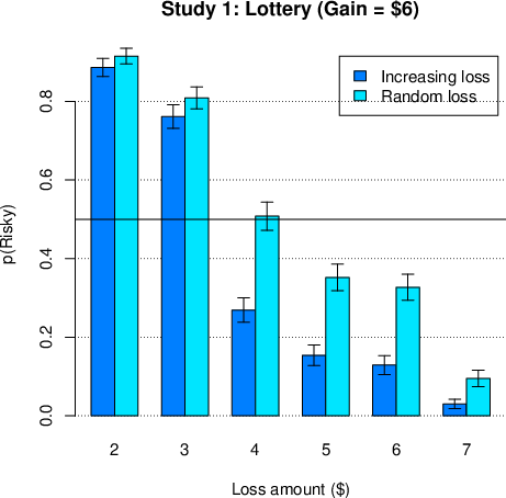
The mean responses to the different items in the two tasks are shown in Figure 1 top panel. As can be seen in the figure, participants were highly sensitive to the gains/losses ratio despite the hypothetical nature of the task, and modified their answer in accordance by varying their risk taking level, from 6% when losses were high to about 94% when they were small.

---

  

λ

Figure 1: Top: Study 1 results (replication of Mrkva et al., 2020). Top panel: Proportion of individuals selecting the risky option in the lottery and investment task as a function of the order condition (increasing versus random losses) and size of losses (error terms denote standard errors). Bottom: Violin plots displaying the distribution of λ in Study 1. Wider areas of each violin indicate more participants with that λ coefficient. Box plots display the median (horizontal dark line) and interquartile range for each study. All study conditions had median λ well over 1.

---

2.2.1 Lottery task

Across conditions, for the symmetric gain-loss lottery task, only 22.8% of the participants selected the risky option, which is significantly lower than 50% (binomial test p < 0.001). This replicates Mrkva et al.’s (2020) findings that have led to their conclusion that loss aversion emerges even for small losses. Our modeling analysis similarly revealed that for the lottery task, the average λ was 1.46 (with a median of 1.50; see Figure 1 bottom panel).

Examining the effect of item order, we find that, on average, participants took significantly more risk when items were randomized than when losses were increasing (t(398) = 5.21, p < .001). The average λ in the increasing losses condition was 1.59 compared to only 1.32 in the random loss condition (the respective medians were 1.50 and 1.20). Therefore, steadily increasing losses biased participants in the direction of loss aversion.

2.2.2 Investment task

For the item with symmetric gains and losses (of $100), only 6.8% of the participants selected the investment, which appears to be consistent with loss aversion (binomial test p < .001). Modeling revealed a corresponding average λ of 2.38 (median λ = 2.00). In this task, the effect of random order was not significant (t(398) = 0.44, p = .33).

2.2.3 Additional effects

There was no effect of gender on the estimated λ in the lottery task (t(360) = 1.85, p = .07) but there was a significant effect in the investment task (t(384) = 3.45, p < .001), with men having lower estimated loss aversion in this task.⁷ With respect to age, however, there was no correlation in either task (Lottery: r = -0.01, p = .80: Investment: r = -0.03, p = .59), which does not replicate the results of Mrkva et al. (2020) that older individuals tend to be more loss averse. We also did not replicate the correlation between λ and ranked education in either task (r = 0.07, p = .19; r = 0.03, p =.56, respectively).

3 Study 2: Symmetric random items and the effect of accept/reject framing

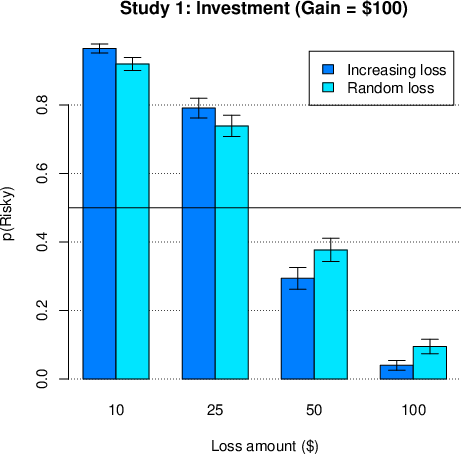
In this study and in the remaining studies the lottery and investment tasks were modified such that losses were symmetric in terms of their distance above and below the gain outcomes. For instance, the lottery task (shown in Table 1) produced a win of $6 and a loss of either $4, $5, $6, $7, or $8. In this symmetric task, random noise does not bias towards loss aversion. We used the version of Study 1 where the order of the items was randomly determined for each participant. Finally, we manipulated the possible strength of the status quo effect. Though the instructions for the two tasks were the same (see below), in one condition participants were given choices between accepting and rejecting the lottery. In this accept/reject framing the status quo is that one does not possess the lottery (i.e., reject). In the alternative choice-framing condition participants were given a choice between getting the lottery and getting zero, and thus the status quo was less clear. Accordingly, we examined whether a task with balanced gains and losses and random order would eliminate the loss aversion observed for small losses; and also evaluated the potential influence of the status quo effect.

---

Table 1: Outcomes in the lottery and investment task used in Study 2. Gains and losses were presented with equal (50%) probabilities. The lottery task was also used in Studies 5 and 6.

Item	Lottery (gain/loss)	Investment (gain/loss)
1	$6 / –$4	$100 / –$25
2.	$6 / –$5	$100 / –$50
3.	$6 / –$6	$100 / –$100
4.	$6 / –$7	$100 / –$150
5.	$6 / –$8	$100 / –$175

---

3.1 Method

3.1.1 Participants

We recruited 401 Prolific Academic participants (193 females, 202 males, 6 other) to take part in this study. Their average age was 34.6 (SD = 12.9). From this sample, 201 participants were randomly allocated to the accept/reject framing condition and 200 were allocated to the choice framing condition. Participants in both conditions received a fee of $1 for completing the study.

3.1.2 Task

The revised lotteries for both tasks appear in Table 1. Items were presented randomly. Task instructions were as in Study 1, with the complete instructions available in Appendix A. In the accept/reject framing condition the lottery was shown in one line (e.g., “If the coin turns up head, then you lose $6; if the coin turns up tails, then you win $6”) while the response, shown in the line below, was either “Accept” or “Reject”. In the choice framing condition the first line indicated “Choose one of the options” and in the response line below participant selected between the lottery (e.g., “50% chance to lose $6 and 50% chance to win $6”) and an option of getting zero (i.e., “get 0”). As in Study 1, each item was presented on a separate screen, and the two tasks included 10 items. After completing the two tasks participants filled in demographic and financial questionnaires (see supplementary section). Modeling analyses were conducted as in Study 1.

---

  

  

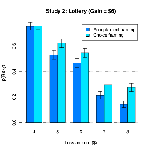
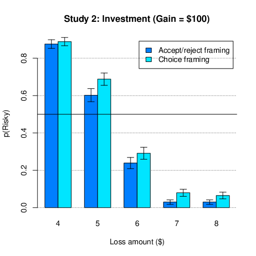
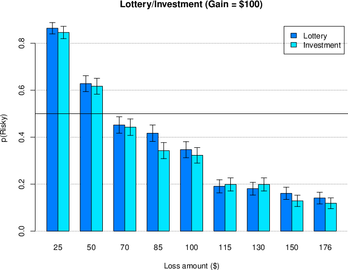
Figure 2: Study 2, 5, and 6 results using symmetric items. Proportion of individuals selecting the risky option in the lottery and investment task as a function of the framing condition (accept/reject vs. choice framing) and size of losses. Error terms denote standard errors.

---

3.2 Results

The mean responses to the different items in the two tasks are shown in Figure 2 top panel. As in the previous study, participants were highly sensitive to the gains/losses ratio and on average modified their risk-taking level monotonically with the size of the loss.

3.2.1 Lottery task

Across conditions, in this symmetric gain-loss task version, 50.7% of the participants picked the risky option, which is not significantly different from 50% (binomial test p = .80), and indicates gain-loss neutrality. Consistently with this, our modeling analysis revealed that the average λ was 0.92 (the median was 1.0; see Figure 3). The effect of the accept/reject framing was in the direction of loss aversion (t(398) = 2.33, p = .02). The average λ for the accept\reject framing was 1.00, while for the choice framing it was 0.84 (respective medians were 1.00 and 0.86).

---

λ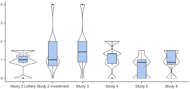

Figure 3: Violin plots displaying the distribution of λ in Studies 2-6. Wider areas of each violin indicate more participants with that λ coefficient. Box plots provide the median (horizontal dark line) and interquartile range for each study. The median Lamda approached 1 in the lottery task in Study 2, 5, and 6 in which symmetric small losses and gains were used. Also, in Study 4 with a moderate loss of $40, only about half (51%) of the participants had λ above 1.

---

:

3.2.2 Investment task

For the item producing a loss and a gain of $100, 27% of the participants selected the investment, which is somewhat higher than in Study 1, though still consistent with loss aversion (binomial test p < .001). Modeling revealed an average λ of 1.45 (median λ = 1.00; see Figure 3). The lower median is partially due to the low granularity of the task; namely most participants rejected the symmetric loss/gain investment but accepted the one with a somewhat lower loss. Again, the effect of the accept/reject framing was in the direction of loss aversion for all lotteries (t(398) = 2.19, p = .03) denoting the biasing effect of this phrasing.

3.2.3 Additional effects

As in Study 1, we observe no effect of gender on λ estimated in the lottery task (t(338) = 0.33, p = .74) while in the investment task we do find an effect of gender (t(378) = 2.41, p < .02), with men having lower loss aversion estimates.⁸ With respect to age, we find no significant correlation for the lottery task (r = 0.03, p = .63) but a weak correlation for the investment task (r = 0.11, p = .04), thus partially replicating the correlation found in Mrkva et al. (2020). For conciseness, similar analyses in all subsequent studies are included in the supplementary section and summed up in the general discussion.

4 Study 3: High stake lotteries versus investments

In Study 2 we found loss aversion in the investment task and no loss aversion in the lottery task when using symmetrical items. There are two main differences between the two tasks: the first is the size of the outcomes, and other is the framing of the task as lotteries versus investment. Possibly, participants in an investment context want to feel that they gain money rather than stay even (Shang, Duan & Lu, 2021), and for this reason may be more loss averse in this task. We therefore manipulated the task context to involve either a risky lottery or an investment. The payoffs used in the current study were those of the (revised) investment task used in Study 2. In addition, because in Study 2 it was difficult to characterize the median of the loss aversion parameter, we added items so that there was a finer grain of losses (as shown in Table 2).

---

Table 2: Outcomes in the lottery and investment task used in Study 3 and 4. Gains and losses were presented with equal (50%) probabilities. Outcomes in Studies 3 and 4 were presented as either lotteries or investments (in two conditions).

	Study 3 (large losses)	Study 4 (moderate losses)
Item	(gain/loss)	(gain/loss)
1	$100 / –$25	$40 / –$20
2.	$100 / –$50	$40 / –$30
3.	$100 / –$70	$40 / –$40
4.	$100 / –$85	$40 / –$50
5.	$100 / –$100	$40 / –$60
6.	$100 / –$115	$20 / –$20
7.	$100 / –$130	$10 / –$10
8.	$100 / –$150
9	$100 / –$175

---

4.1 Method

4.1.1 Participants

A total of 400 participants (219 females, 174 males, 7 other) volunteered to take part in the study. Their average age was 35.8 (SD = 13.5). From these participants, 201 individuals were randomly allocated to the investment condition and the remaining 199 were allocated to the lottery condition. Participants in both conditions received a fee of $1 for completing the study.

4.1.2 Task and analysis

The study included a single task which was performed using either the instructions of the lottery task or those of the investment task (see Appendix A). Task outcomes are shown in Table 2. As in Study 2, the order of the items was randomized for each participant. Items were administered using the choice-framing format, namely with the first line in each item indicating “Choose one of the options” and the response line below involving a selection between the lottery or the investment and getting zero (e.g., “50% chance you could win $100 and 50% chance you could lose $25” or “get 0”). As previously, following the main task participants completed a short demographic test (see supplementary section). Analyses were conducted as in the previous studies.

4.2 Results

The mean responses to the different items are summarized in Figure 4. As evident in the figure, participants again seemed to be sensitive to the size of gains and losses. They also seemed to be relatively unaffected by whether the task involved lotteries or investments. Across task conditions, only 33.5% of the participants select the risky option with symmetric gains and losses, which was significantly below 50% (binomial test p < .001)), thus replicating our results in Study 2. Modeling analyses revealed an average λ of 1.64 (median of 1.43; see Figure 3). Participants came closest to equal rates of risky and safe choices when the gain was $100 and the loss was $70 (in this case 44.8% picked the risky option, slightly differing from 50%; binomial test p = .04). When examining the effect of task type we find no significant difference across items (t(398) = 0.62, p = .40). Thus, we find that it is not the investment context that produces what appears like loss aversion for high amounts, but rather the magnitude of losses. High magnitudes provide sufficient conditions for the emergence of a loss-aversion like behavior. An examination of gender and age differences appears in the supplementary section.

---

Figure 4: Study 3 results. Proportion of individuals selecting the risky option in the lottery/investment tasks as a function of the size of the loss. Error terms denote standard errors.

---

5 Study 4: Moderate losses

One could argue that the absence of loss aversion only emerges for the small loss of $6 in the lottery task but not for less trivial losses. In this study we examined lotteries with symmetric gains and losses of either $10, $20, and $40, along with items with varying gains and losses, as shown in Table 2. Specifically, outcomes in the investment task used in Study 2 were reduced by a factor of 2.5 (resulting in a mean loss of $40), and two items were added with symmetric gains and losses of $10 and $20. For robustness, we administered the task as either a lottery or an investment task (as in Study 3).

5.1 Method

5.1.1 Participants

A total of 400 participants (218 females, 180 males, 2 other) took part in the study. Their average age was 37.7 (SD = 14.1). From these individuals, 200 were randomly allocated to the investment task and 200 to the lottery task. Participants in both conditions received a fee of $1 for completing the study.

5.1.2 Task and analysis

As in the previous study, participants completed a single task which was performed either with the instructions of the lottery task or the investment task (see Appendix A). Task payoffs appear in Table 2. Items were administered using the choice-framing format, and in random order. This task was followed by a short demographic survey (see supplementary section). The analysis was as in the previous studies, though we separately examined the response to items with symmetric gain/loss magnitudes ($10, $20, $40) in order to evaluate the effect of payoff size. In the modeling analysis we only included items with varying gains presented for the same loss ($40).

5.2 Results:

Mean responses to the different items are summarized in Figure 5. As can be seen, participants’ tendency to avoid the risky lottery depended on the magnitude of gains and losses. Again, our initial focus was on the lotteries with symmetric gains and losses. When responding to the $40 gain/loss item, only 34.5% of the participants selected the risky option, significantly below 50% (binomial test p < .001). However, for the item with a gain/loss of $20, 49.8% of the participants preferred the risky option (binomial test p = .96), while for the $10 loss/gain 63.8% preferred to take risk (binomial test p < .001, above 50%). Thus, behavioral indications of loss aversion started to emerge only for losses of $40.

---

Figure 5: Study 4 results. Proportion of individuals selecting the risky option in the lottery/investment tasks as a function of the size of gains and losses. Error terms denote standard errors.

---

Focusing on the items with a fixed $40 gain and a mean $40 loss, our modeling analysis reveals an average λ of 1.16 (median of 1.33; see Figure 2), which is rather low in comparison to previous estimates (e.g., Mrkva et al., 2020). Indeed, for the average $40 loss only 51.0% of the participants had λ above 1. For the $20 loss the best proxy of the mean λ appears to be 1.0 (given the proximity of choices to preference neutrality), while for the amount of $10, λ seems to fall well below this value (though we cannot estimate it using the current task). Finally, there was no effect of task type on choices across items (t(398) = 0.96, p = .34), showing that the current results are robust to task instructions.

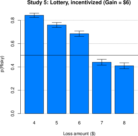
6 Study 5: Effect of incentivization

In Studies 2 and 4 we find that for lotteries and investments with small gains and losses, up to $20, individuals do not display loss aversion. However, one might argue that this is due to the fact that gains and losses in our previous studies were not incentivized. Though Mrkva et al. (2020) also did not incentivize participants in the lottery and investment tasks, one might argue that hypothetical losses produce different response from actual losses (e.g., Holt & Laury, 2002). We therefore aimed to evaluate whether for small incentivized lotteries as well, individuals do not exhibit loss aversion. For this purpose, we used an incentivized version of the lottery task in Study 2 (see Table 1).

6.1 Method

6.1.1 Participants

A total of 400 participants (230 females, 166 males, 4 other) took part in the study. Their average age was 36.5 (SD = 13.8). Participants received a fee ranging between $1 to $15 for completing the study, based on their choices and the realization of the lotteries. Specifically, there was a $1 participation fee while the remaining amount was based on participants’ choices and the realization of a randomly selected lottery.

6.1.2 Task and analysis

In this study all participants performed the lottery task. Items were administered using the choice-framing format, and in random order. The only difference between the current study and the choice-framing condition of Study 2, is that choices were incentivized. Specifically, participants were initially informed that in addition to their participation fee of $1, an amount of $8 would be deposited at their temporary account, and that at the end of the task the temporary account will be added to their participation fee. Also, as part of the lottery/ investment task instructions, participants were informed that one of the lotteries/investments will be randomly selected and based on their choice it will be either played or not, and that any resulting gains or losses will affect their temporary account (see complete instructions in Appendix A).

6.2 Results

The mean responses to the different items are summarized in Figure 2 bottom left panel. For symmetric gains and losses of $6, we find that 68.5% of the participants preferred the lottery over the safe option, significantly above 50% (binomial test p < .001). Our modeling analysis indicated an average λ of 0.64 (median of 0.86; see Figure 3) which denotes gain seeking (opposite of loss aversion). Most participants (68.8%) had λ estimates below 1. Furthermore, the lottery where responses were closest to 50% involved a gain of $6 and a loss of $7. Only 56% of the participants avoided this lottery (binomial test p = .02). Our results thus show that incentivization did not produce loss aversion.

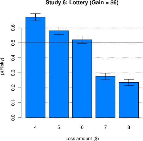
7 Study 6: Relationship with the endowment effect

In our final study we leave our main focus on the weighing of gains and losses, and examine the relationship between risk taking for gains and losses and valuation of objects. Mrkva et al. (2020) argued that, if both risk aversion and the endowment effect are driven by loss aversion, the two behavioral phenomena should correlate positively. This was strongly supported in their study with a positive correlation of 0.55 between the extra surplus an individual charged as a seller compared to a buyer, and the loss aversion parameter estimated for risky lotteries. However, an alternative account is that the correlation is due to the same “subject misconceptions” (to borrow a term used by Plott & Zeiler, 2005) by the same individuals in both tasks. Particularly, since both tasks in Mrkva et al. (2020) adopted the same paradigm of steadily and monotonically increasing costs, the correlation could be due to the resulting tendency of some individuals to treat items inter-relatedly (see footnote 4). We therefore supplemented the lottery task with a buying and a selling task. As in Mrkva et al. (2020) participants performed one task at the beginning of the experiment and at the other at the end, with counter-balanced order. However, while the buying and selling tasks used monotonically increasing prices as in Mrkva et al. (2020), our risk-taking task involved randomly presented gains and losses as in Study 2-5. Another difference was that Mrkva et al. (2020) used a physical object (car model) as the endowed object, while we used a lottery ticket. A recent meta-analysis evidenced strong endowment effects for lottery tickets similar to those observed for other commodities (Yechiam, Ashby & Pachur, 2017).

7.1 Method

7.1.1 Participants

A total of 400 participants (196 females, 198 males, 6 other) took part in the study. Participants were randomly allocated into two order conditions. Two- hundred performed the selling task first and the buying task last, and 200 performed the tasks in reverse order. Participants’ average age was 35.5 (SD = 13.2). They received a fee ranging from $1 to $1.6 based on their choices and the realization of the lotteries in the buying/selling tasks. Specifically, there was a $1 participation fee and the remaining amount was based on their choices.

7.1.2 Task

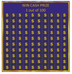
The initial task was either a buying or a selling task. In the selling task participants were informed that they are given a lottery ticket with a 1/100 chance to win 20 experimental dollars which they could keep or sell to the organizers of the study. In the buying condition participants had the opportunity to buy the same lottery ticket. The instructions for both conditions were adopted from Mrkva et al. (2020) and appear in Appendix B. Importantly, as in Mrkva et al. (2020) participants were incentivized for their buying/selling decisions, with a conversion rate of $1 for each 100 experimental dollars. The initial buying/selling task was followed by the lottery task which was administered with choice framing and random order of items, and was not incentivized, as in Mrkva et al. (2020). Next, participants completed a demographic questionnaire, and a longer financial survey (from Mrkva et al., 2020; see our supplemen) that was used as a filler, followed by the remaining selling/buying task.

7.1.3 Analysis

We calculated selling and buying prices for all participants based on the lowest price which sellers agreed to sell, and the highest price that buyers agreed to buy. We also conducted an analysis in which we removed buyers and sellers who exhibited inconsistent responses (e.g., selling in a certain price but then refusing to sell given a higher price). We first tested whether there was an endowment effect by using a repeated-measures ANOVA with condition (buying/selling) and task order as within-subject factors. Next, we calculated each individual’s selling premium by deducting each individual’s buying price from their selling price. We then replicated our examination of loss aversion in the lottery task as in the previous studies. Finally, we examined the correlation between the selling premium and choices in the lottery task as well as the estimated λ parameter.

7.2 Results

Participants’ mean selling price (i.e., willingness to accept price; WTA) was $4.28 (SE = 0.16), compared to a mean buying price (i.e., willingness to pay; WTP) of $2.47 (SE = 0.11), denoting a 1.73 relative increase in selling estimates. An ANOVA examining the endowment effect and the order of the buying/selling task showed that the selling premium was significantly above zero, F(1,398) = 109.50, p < .001). The effect of the task order was also significant (F(1,398) = 12.16, p < .001), with higher valuations for those initially allocated to the selling conditions: On average $5.66 (SE = 0.15) compared to 4.51 (SE = 0.15) for those who bought first.

The results of the lottery task are shown in Figure 2 bottom right panel. As can be seen, we replicate our finding of no behavioral loss aversion for the item with symmetric gains and losses. For this item, 52.0% of the participants picked the risky lottery (binomial test p = .45). An estimation of λ conducted as in the previous studies revealed a mean λ of 0.91 (median of 0.86; see Figure 3).

We next examined the correlation between the selling premium and risk taking in the lottery task as the individual level. We first focused on the mean tendency to avoid losses across lotteries. We recover a correlation of 0.17 (p < .001) between the endowment effect and avoidance of the lotteries. We thus replicate the positive correlation observed in Mrkva et al. (2020) though in our study it is considerably smaller. Indeed, behavioral responses to the gain-loss lotteries account for only 2.9% of the variance in the selling premium. We find a similar correlation between the selling premium and λ (r = 0.16, p = .001).

We also conducted a robustness test that focused on individuals who performed the selling and buying task without any inconsistencies. This removed 14% of the selling estimates and 21.5% of the buying estimates (the greater coherence of selling price is consistent with that found in other studies; see Yechiam et al., 2017). The results for this subset showed a significant endowment effect, with a mean selling price of $4.75 compared to a buying price of $2.95 (F(1,276) = 79.36, p < .001) and again a small positive correlation between risk avoidance in the lottery task and the selling premium, r = 0.20, p < .001.

8 An analysis of first presentation effects

One might argue that the design of the current studies involving multiple items could bias responses towards loss neutrality despite the balanced range of expected values and random order, because some items are typically presented before the target lotteries with equal-sized gains and losses. Thus, it was important to examine these key lotteries when presented first. To evaluate this, we examined the responses to the lotteries involving same sized gains and losses when these were administered as the first lotteries (to about 1/k of the participants, where k is the number of items which ranged from 5 to 9 in different studies), or not. The results are presented in Figure 6, and relevant statistical analyses appear in the supplemen. As can be seen, in all studies across key lotteries, the results trended in the direction of lower loss aversion when these items were presented first. A statistical analysis, available in the supplementary section, shows that this effect was significant in some of the studies, and that it consistently emerged when the loss amount was small ($6). Interestingly, in Study 1 which uses Mrkva et al.’s original task conditions, when the item with symmetric gains and losses of $6 is presented first, eliminating the effect of asymmetrical outcome sizes and any type of order effect, participants also did not significantly avoid the lottery (53% chose to enter the lottery; see supplementary section). Importantly, these results do not imply that those who were not presented with the target prospects first, showed loss aversion for smaller amounts (except in Study 1 which replicated Mrkva et al.’s task conditions). The rate of those who were presented with these key prospects first was relatively small and therefore removing these participants from the sample does not markedly change the results reported in our main analysis, as shown in Figure 6 and analyzed in the supplementary section.

---

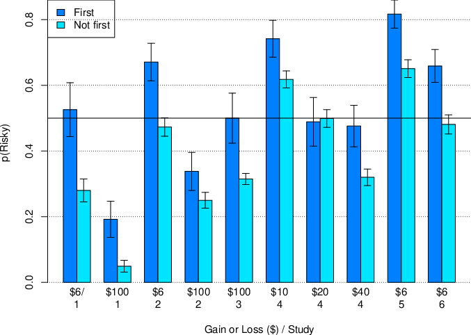
Figure 6: First-presentation effects in the studies in which the order of the lotteries was randomized (Study 1 random-order condition, and Studies 2-6). Proportion of individuals selecting the risky option in the lottery/investment tasks in items with identical-sized gains and losses, as a function of whether it was the first presented lottery or not, and given different sizes of (identical) gains and losses. Error terms denote standard errors.

---

9 Discussion

Our first study showed that Mrkva et al.’s (2020) findings of apparent loss aversion for small losses are replicable in online participants. However, our next set of five studies show that they are driven by design features in the list method used by Mrkva et al. (2020) and others (e.g., Tversky & Kahneman, 1992), especially the non-symmetric gains and losses and non-random order. In Studies 2–6 we find that when gains and loss items are symmetrical, namely when the average loss is equal to the average gain, and items are administered randomly, individuals do not behave in a strong loss-averse manner unless the losses are high (around $100). Specifically, for average losses of up to $20 participants did not show loss aversion, even in a condition when they were incentivized. For an average loss of $40 participants showed weak loss aversion with a mean λ of 1.16 and with only 51% of the participants having λ estimates above 1. In tasks with higher losses averaging $100, we do observe what appears to be loss aversion. Yet even in these higher stakes lotteries/investments, our estimate of λ for symmetric items is not as high as in previous studies (e.g., Tversky & Kahneman, 1992; Mrkva et al., 2020), with a mean λ of 1.54 across studies. This indicates that differently from the notion espoused in prospect theory, the λ coefficient is not constant across different loss amount, but instead is highly dependent on the amount, and goes to 1 or below for smaller amounts.

Our findings also show that a variety of task-related factors can bias participants to behave in an apparent loss averse manner. As noted at the outset these factors include: a) items with asymmetric sizes of gains and losses, b) monotonically increasing/decreasing loss amounts which may lead to perceived inter-item relationships, and c) the usage of an accept/reject framing for possible options. In Study 1 we found a notable effect of randomizing items. Even given non-symmetrical gains and losses, randomizing items reduced loss aversion by about half (from λ of 1.59 to 1.32, on average). In Study 2 we found that changing the asymmetric loss/gain items to symmetrical ones and randomizing item order provided sufficient conditions for the complete disappearance of loss aversion with small losses. In this study we also found that not using an accept/reject framing further reduces loss aversion. By contrast, a factor that was not found to affect choices (in Studies 3–4) is the framing of the task as a lottery or an investment (Shang et al., 2021).

Our analysis of order effects in all studies indicated that loss aversion in symmetric gain/loss lotteries was apparently further reduced when small-sized lotteries were presented first. This is consistent with Ert and Erev’s (2013) finding that loss aversion was lower when tasks are relatively simple, though they did not find a significant order effect in their study. This first-presentation effect is an interesting and hitherto unobserved moderator of people’s sensitivity to losses.

In addition, our final study examined the relationship between the sensitivity to gains and losses in lotteries and the endowment effect. To our surprise, we did find a small positive correlation between these indices, consistently with Mrkva et al. (2020). The correlation admittedly could be weak because the two measures are noisy and not necessarily because they are unrelated. This suggests that the weighting of gains and losses may be implicated to some degree in both phenomena at the individual level. However, it is quite erroneous to extrapolate from these findings that loss aversion “drives” both phenomena at the population level. Simultaneously with the positive correlation at the individual level, we found no loss aversion for the average participant in the lottery task compared to a huge endowment effect for the same participants. Moreover, the endowment effect was observed for a lottery with a moderate amount (nominal outcome of $20) for which no loss aversion emerged in our studies. Thus, it does not seem to make sense to refer to the same construct as underlying both phenomena.

We also do not replicate the correlation with age and education observed by Mrkva et al. (2020) consistently across studies. In particular, as detailed in the supplementary section, the positive correlation between loss aversion and age appeared only sporadically, in one of our studies. The only consistent individual difference factor affecting choices was gender, but its effect was not coherent across payoff magnitudes, being present only for risks involving large losses. This again emphasizes the fact that the loss aversion parameter is not stable given different payoff magnitudes.

Notice that some of these effects can be captured by expected utility theory (von Neumann & Morgenstern, 1944). Most especially the absence of loss aversion for small amounts and increased risk aversion with stake size can be captured if one assumes a certain wealth level to which outcomes are added, and a diminishing marginal utility of wealth (Hansson, 1988). Indeed, the current findings seem to reconcile (or at least alleviate) the paradoxical EU theory predictions implied by assuming loss aversion for lower losses (Hansson, 1988; Rabin, 2000). However, other aspects of our findings, such as the reduced loss aversion with random order, and the first presentation effect, violate the procedural invariance assumption of expect utility theory. Also, another implication of risk aversion contingent on wealth level which does not emerge in our data, is that (in approximation) loss aversion should be sensitive to one’s income (similarly, Mrkva et al., 2020 also found inconsistent correlations between income and loss aversion in their studies).

Limitations of our study include the reliance on online participants from Prolific Academic, namely individuals who have experience in engaging in behavioral experiments. One could ask whether for these individuals, our presentation of potential losses or even actual losses in Study 5 was sufficient to produce the same kind of feeling one gets when losing money out of one’s own wallet. A further limitation is our usage of a fixed text of “get $0” for the outcomes of the safe alternative, which may have been unattractive to the participants. While we cannot directly address these issues with the current dataset (and indeed the former is difficult to examine without some ethical issues), we can say that we do replicate in this population and paradigm the very high degrees of loss aversion found in Mrkva et al. (2020) when we use the exact same conditions of their study: non-symmetric gains and losses, an order effect, and a status quo effect.⁹ Still, we realize further studies should validate the possibility that experience in participation in decision making studies, particularly online, might alleviate the loss aversion tendency.

To sum, when using non-symmetric items we do replicate Mrkva et al.’s (2020) results of “loss aversion” even for small amounts and in an online sample, but using balanced symmetric gains and losses and random items this is not replicated. Instead, we find that loss aversion does not emerge for small amounts and emerges very weakly for a moderate amount ($40). This finding has important ramifications to the question for whether loss aversion exists. As aptly noted by Mrkva et al. (2020), a critical implication of loss aversion is that for small amounts as well individuals overweigh losses compared to gains. Moreover, loss aversion implies that the ratio of inflating losses over gains should be constant over different amounts. The findings that loss aversion does not emerge for small losses and is much weaker for moderate losses suggest that there is no grand simple explanation related to the subjective weighting of gains and losses across different amounts. We hope that new models are developed to account for these findings.

10 References

Appendix A: Lottery and investment task instructions

General instructions

In this study, you will answer a brief survey including some demographic questions as well as some questions about hypothetical preferences. The duration of the study will be about 5-7 minutes. In return for completing the survey, you will be awarded $1.

Study 5/6: In addition, an amount of $8/$0.2 is deposited at your temporary account. This amount may increase or decrease depending on your choices during the study. At the end of the task, your temporary account will be added to your $1 participation fee, and your final fee will be $1 to $15/$1.6.

Lottery task

Suppose you were offered an opportunity to enter a lottery based on a toss of a fair coin. If the coin turns up heads, you lose some money; if it turns tails, you win some money. Please indicate for each lottery whether you would ’accept’ that is play the lottery, for a chance of winning or ’reject’ it and not receive anything.

Investment task

Suppose you were offered an opportunity to make an investment where you had a 50% chance of winning $100¹⁰ and a 50% chance of losing various set amounts. Would you make any of the following investments?

Study 5 (only): One of the lotteries/investments will be randomly selected and based on your choice it will be either not played (and you will get 0 for it) or played with a virtual coin having 50% chance of turning either heads or tails. The resulting gains or losses will be added to/ deducted from your temporary account.

Appendix B: Incentivized buying and selling instructions

Buying task

We will offer you the chance to buy the following lottery ticket with a 1/100 chance to win 20 Experimental Dollars. This lottery ticket can be yours! If you want to acquire this lottery ticket, you can buy it from the organizers. Please indicate below for each respective price if you are ready to buy the lottery ticket.

• If at the price for which we sell the lottery ticket to you, you have indicated that you are ready to buy, you will receive the lottery ticket from us at this price, which you have to pay to us. Then we will inform you whether the lottery ticket won.

• If at the price for which we sell the lottery ticket to you, you have indicated that you are not ready to buy, you do not receive the lottery ticket.

The price at which we will sell the lottery ticket to you will be randomly determined by us and for sure be between 0 and 10 Experimental dollars. That is, our selling price will be determined by rolling dice after you have filled in the table. All prices are equally likely.

Since you cannot influence the selling price, which we will determine randomly, you have an incentive to state the price that corresponds to your true preference.

Once you have made your choice, you cannot change it anymore. We are also not able to negotiate the randomly determined selling price.

For each 100 experimental dollars, you gain/ lose $1 (actual dollars) and this will be added/ deducted from your fixed amount of $1.2 (actual dollar) earning for the experiment.

If the price is $X¹¹

o I am ready to buy

o I am not ready to buy

Selling task

We will give you the following lottery ticket with a 1/100 chance to win 20 Experimental dollars which you can keep. This lottery ticket is yours! If you do not want to keep the lottery ticket, you can sell it to the organizers of this study. Please indicate below for each respective price if you are ready to sell the lottery ticket.

• If at the price for which we buy the lottery ticket from you, you have indicated that you are ready to sell, you will receive this amount of experimental dollars instead of the lottery ticket.

• If at the price for which we buy the lottery ticket from you, you have indicated that you are not ready to sell, you will keep your lottery ticket and one lottery outcome will be randomly selected at the end of the study.

The price at which we will buy your lottery ticket will be randomly determined by us and for sure be between 0 and 10 Experimental dollars. That is, our buying price will be determined by rolling dice after you have filled in the information below. All prices are equally likely.

Since you cannot influence the buying price, which we will determine randomly, you have an incentive to state the price that corresponds to your true preference. Once you have made your choice, you cannot change it anymore. We will also not be able to negotiate the randomly determined buying price.

For each 100 experimental dollars, you gain/ lose $1 (actual dollars) and this will be added/ deducted from your fixed amount of $1.2 (actual dollar) earning for the experiment.

If the price is $X¹²

o I am ready to sell

o I am not ready to sell

*

Technion – Israel Institute of Technology, Faculty of Industrial Engineering and Management, https://orcid.org/0000-0002-6415-3562.

#

Technion – Israel Institute of Technology, Faculty of Industrial Engineering and Management, https://orcid.org/0000-0003-0389-2131. E-mail: yeldad@ie.technion.ac.il

Copyright: © 2022. The authors license this article under the terms of the Creative Commons Attribution 4.0 License.

1

For instance, λ of 2 implies that a loss is given twice the weight of a respective gain, while λ of 1 denotes gain-loss neutrality.

2

For example, as demonstrated by Rabin (2000), an expected-utility maximizer who always turns down 50–50 lose $10/gain $11 bets will always turn down ones where you lose $100 or can gain any sum of money with equal probability, simply because under expected utility theory risk aversion increases with the lottery outcomes. More generally, Hansson’s (1988) and Rabin’s (2000) critique concerns “first order risk aversion” models which allow for risk-averse behavior even if the stakes are small (Segal & Spivak, 1990; and see also O’Donoghue & Somerville, 2018).

3

Mrkva et al. (2020) note this possible confound but argue that findings of loss aversion are also replicated in other papers with no status quo effect.

4

Namely, such strategic participants would opt for the lottery producing the lowest losses (thus displaying “loss aversion”), sell for the highest price, and buy for the lowest price (thus exhibiting an “endowment effect”).

5

The number of participants in all studies was set to 400. Specifically, we ran 300 participants, checked the gender ratio, and set a gender ratio for the next 100 participants that would increase equal gender representation.

6

For example, assume a questionnaire with only two items: a symmetric equiprobable gain and loss lottery of $100, and one with a gain of $100 and a loss of $50. If the majority rejects the former and accepts the latter gamble, and if this implies an orthodox λ of 1 (using the specifications of prospect theory as in the main text above), then the median λ will be 1 while the mean will be higher and thus more representative.

7

When examining risk taking across items the effect of gender is significant in both the lottery task (t(394) = 2.55, p = .01) and the investment task (t(394) = 4.35, p < .001).

8

Again, this is also replicated for choices across lotteries and investments (t(393) = 0.14, p = .44; t(393) = 2.58, p = .005; respectively).

9

Moreover, in an unpublished study, Argaman, Ludvig and Yechiam (2020) avoided the “$0” notation by presenting Prolific Academic participants with an image of a scratch card described as having a 7/100 odds of winning $5, 7/100 odds of losing $5, and 86/100 odds of 0 (neither win nor lose). Two-hundred participants were asked to indicate what they would do if they had to choose between playing the scratch card with real gains and losses, or playing it for no money (neither gaining nor losing money). Fifty-nine percent chose to play for real money (see data in https://osf.io/5xdrf/).

10

In Study 4 this was changed to “wining an amount of money”.

11

In each of 20 items X was steadily increased from 0 to $10.

12

In each of 20 items X was steadily increased from 0 to $10.

This document was translated from L^AT_EX by H^EV^EA.