Judgment and Decision Making, Vol. 17, No. 5, September 2022, pp. 988-1014
The endowment effect in the future: How time shapes buying and selling prices
Shohei Yamamoto*
Daniel Navarro-Martinez#
|
Abstract:
Previous research has focused on studying the endowment effect for
transactions that take place in the present. Many real-world transactions,
however, are delayed into the future (i.e., people agree to buy or sell,
but the actual transaction does not materialize until a later time). Here
we investigate how transaction timing affects the endowment effect. In
five studies, we show that the endowment effect systematically increases
as transactions are delayed into the future. Specifically, buying prices
significantly decrease as the transaction is delayed, while selling prices
remain constant, resulting in an amplified endowment effect (Experiment
1). This pattern is not produced by a discounting of the money involved in
the transaction (Experiment 2), and it holds across different types of
items (Experiment 3). We also show that the phenomenon cannot be explained
by sellers anticipating becoming increasingly attached to the items over
time (Experiment 4). Finally, we demonstrate that this increased endowment
effect in the future holds in the field, in the context of a real market
and with real transactions (Experiment 5).
Keywords: endowment effect, intertemporal choice, choice delay
1 Introduction
It has been widely documented that, when people are endowed with an item,
they ask for a greater compensation to give it up than they would be
willing to pay to acquire it. This pattern has been called the
endowment effect (Thaler, 1980) and it is one of the most prominent
phenomena in judgment and decision making, with important implications for
a variety of situations related to buying, selling and evaluating
resources (for reviews, see Horowitz & McConnell, 2002; Kahneman et al.,
1991; Tunçel & Hammitt, 2014). However, virtually all research on the
endowment effect has investigated transactions that take place in the
present (i.e., buying or selling items that will be exchanged here and
now). This is a significant limitation, given that many real-world
transactions have a temporal dimension. In many circumstances, people
agree on a purchase or a sale but the transaction does not materialize
until a later time in the future, for example in almost all forms of
online buying and selling. In this paper, we investigate how delaying
transactions into the future affects the endowment effect.
The endowment effect is often explained in terms of loss aversion (Kahneman
& Tversky, 1979; Tversky & Kahneman, 1991). According to this
explanation, buyers see an item they may acquire as a potential gain,
whereas sellers view the same item they may give up as a potential
loss. Because losses loom larger than gains, this difference creates the
asymmetry between the two parties known as the endowment effect. Many other
explanations and moderating factors have been suggested (see, e.g., Burson
et al., 2013; Georgantzís & Navarro-Martinez, 2010; Johnson et al., 2007;
Morewedge & Giblin, 2015; Morewedge et al., 2009; Plott & Zeiler,
2007). For instance, Johnson et al. (2007) proposed a memory-based account
of the endowment effect, where buyers and seller retrieve different aspects
of the items to produce their valuations. In a different line of research,
Morewedge et al. (2009) suggested that the endowment effect happens
because people associate the things they own to themselves and this in turn
increases their valuations, rather than having an aversion to loses per
se.
The most established way to measure the endowment effect (and the way we
elicit it in this paper) is in terms of willingness to accept (WTA) and
willingness to pay (WTP). In a typical experiment, subjects are
randomly assigned to one of two conditions: one in which they are endowed
with a target item and are asked for their WTA to sell it, and one in
which they are not endowed with the item and are asked for their WTP to
acquire it. WTA is normally higher than WTP, which constitutes the
endowment effect (also called WTA-WTP disparity in this framework).
We find it surprising that few papers have investigated how the endowment
effect, WTA and WTP relate to time, given that
transactions with a temporal component or delay are very common in daily
life. One of the clearest examples of this is arguably online markets such
as Craigslist, eBay or Facebook Marketplace, where people buy and sell
items, typically by agreeing on an exchange sometime in the future (in one
day, one week, one month, etc.). These markets are growing and are home to
billions of transactions of very diverse goods every year. For instance,
Mark Zuckerberg announced at the Facebook 2021 first quarter earnings call
that Facebook Marketplace was used by more than 1 billion people per
month. On all these platforms, the endowment effect, with its associated
reluctance to trade, is likely to make agreements and exchanges between
buyers and sellers more difficult (see Bar-Hillel & Neter, 1996; Kahneman
et al., 1990; Knetsch, 1989). If the endowment effect is mitigated when
transactions are moved into the future, then delaying transactions may be
a way to alleviate these frictions. If, on the other hand, delayed
transactions amplify the endowment effect, then sooner exchanges will
maximize the chances of getting to an agreement. Apart from these markets,
online shopping more generally usually involves time delays, for example
from Amazon or AliExpress, travel agencies, supermarkets, etc. Also
outside the Internet, delayed transactions are widespread. A typical
example would be buying or selling a car. The parties typically agree on
the sale, but then there are several steps before the actual exchange
happens (paperwork, often ordering the car, etc.). The same holds for
countless other items of different types.
There is a small literature that has related gain-loss differences and the
endowment effect to time in different ways, although none (to the best of
our knowledge) in terms how delayed transactions affect the endowment
effect. Several papers have documented the so-called sign effect,
in which gains of money are shown to be discounted in time more than
losses (Frederick et al., 2002; Thaler, 1981). Hardisty and Weber (2009)
investigated this pattern in three different domains (money, the
environment and health), showing that the sign effect holds in all three
but is stronger in the health domain. Molouki et al. (2019) then showed
that the effect is (partly) linked to the emotional reactions experienced
when contemplating the delayed outcomes in the process of waiting for
them. The sign effect, however, has not been studied in the context of the
endowment effect or of the valuation of goods more generally. Loewenstein
(1988) showed that WTP for a cassette recorder decreased as obtaining the
recorder was delayed for one year, but he did not elicit WTA. If the sign
effect holds in the context of the valuation of goods, we should expect an
increasing endowment effect as transactions are delayed, because WTP would
decrease more than WTA.
But goods are different from money because they generate attachment, and
this could interact with time delays in different ways. On the one hand,
there is evidence that people adapt to owning things and get increasingly
attached to their possessions over time (Strahilevitz & Loewenstein,
1998), at least under some circumstances. If people anticipate this
adaptation, this anticipation could magnify the sign effect in the context
of goods, potentially even leading to an increasing WTA as transactions are
delayed. This effect, however, is unlikely to be substantial, given that
people have been shown not to significantly anticipate attachment in
endowment effect situations (Loewenstein & Adler, 1995; Van Boven et al.,
2000).
On the other hand, there is evidence that the endowment effect is linked to
some extent to affective reactions (Peters et al., 2003; Reb & Connolly,
2007; Shu & Peck, 2011; Zhang & Fishbach, 2005), and we know that
affective reactions are much more prevalent in relation to the present
than to the future (Loewenstein, 1996; 2000). This could potentially
undermine the endowment effect when transactions are delayed, by
decreasing WTA. In other words, giving up something one owns might feel
less dramatic if one only has to part from it in the future.
Overall, there is not a clear-cut prediction coming from previous
literature and our research is, in that sense, exploratory. We present
five experiments to investigate how the endowment effect (in terms of WTA
versus WTP) is affected by delaying transactions into the future. In
Experiment 1, we demonstrate that the endowment effect is systematically
amplified as transactions are moved into the future. Buying prices
consistently decrease as transactions are delayed, while selling prices
remain roughly constant, resulting in an increasing WTA-WTP gap.
Experiment 2 shows that this pattern is not a result of discounting the
money involved in the transaction and is largely a feature of moving the
exchange of the item in time. In Experiment 3, we replicate the same
effect across different types of items. Experiment 4 provides evidence
that the phenomenon cannot be explained by sellers anticipating becoming
increasingly attached to the items over time. In Experiment 5, we show
that the same pattern of an increased endowment effect in the future is
obtained in a field environment, in the context of a real market and with
real transactions.
Our experiments provide converging evidence that endowment effects
significantly increase as transactions are delayed, as we see in many
real-world settings, such as online markets. This result suggests that existing
experimental research on the endowment effect may have underestimated its
magnitude in some more realistic environments. This conclusion has important
implications for the design of market institutions. Exchanging goods as
soon as possible might be important to reach agreements between buyers and
sellers.
2 Experiment
1: The Endowment Effect Moves to the Future
Our first study was designed to test how the endowment effect, in terms of
the WTA-WTP gap, changes as transactions are progressively moved into the
future, as it is typically seen in online markets.
2.1 Method
2.1.1 Subjects
We recruited 300 subjects for our experiment via Amazon Mechanical Turk
(50% female, Mage = 38 years, age range: 19–76
years). The study took an average of 5 minutes and 47 seconds to complete
and subjects received a fixed fee of $0.5. We excluded from our
sample one subject who did not enter the code needed to receive
payment.
2.1.2 Design and procedure
Following standard practice in endowment effect experiments, subjects
were randomized into a buyer or a seller condition. In the seller
condition, people were asked to imagine that they had received an item as
a gift, so that they now owned the item. In the buyer condition, they were
asked to imagine that they had the opportunity to buy that same item,
without being endowed with it. The item used in this experiment was a
framed Game of Thrones poster with a retail price of €18.92.
Subjects were then asked to evaluate either selling or buying the
poster (depending on the condition) and making the transaction in the
present and in different future moments. Specifically, the sellers were
asked “what is the minimum amount of money ($X) that you would require to
sell the item and do the exchange (of money and item) [at time t]?”; the
buyers were asked “what is the maximum amount of money ($X) that you
would be willing to pay to buy the item and do the exchange (of money and
item) [at time t]?” The transaction timing [at time t] was either today,
tomorrow, in 1 month, or in 1 year. These four different time scenarios
were randomized within subjects. We also used a graphical display to
clarify the transaction timings (see Figure A1 in the Appendix).
Before responding to each of the four time scenarios, all subjects had
to correctly answer a qualification question to verify they had understood
the task. If subjects chose an incorrect response, this information
was recorded and a pop-up window appeared and warned them that the answer
was wrong. Subjects could not proceed until they answered correctly.
After the main scenarios, subjects were asked how much they liked the
item (on a scale with seven stars) and how strongly they felt ownership of
the item (on a 7-point scale from 0 = not at all to 6 =
very strongly). Finally, they were asked to complete a brief
demographic survey, asking about their gender, age, English level, field
of professional specialization, level of education, native language, and
also how clear the instructions were.1
2.2 Results and discussion
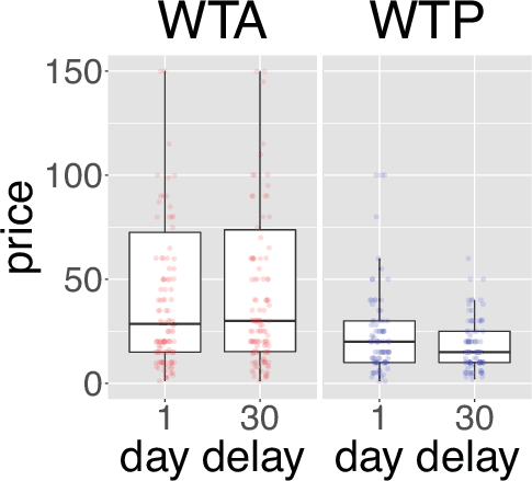
Table 1 reports summary statistics for Experiment 1; Figure 1 presents a
box plot showing the main patterns obtained in WTA and WTP across the
different time scenarios.2
| Table 1: Descriptive Statistics (Experiment 1). |
| | Time | Median | | Mean | | SD | | Total N | Wrong&outliers |
| WTA | Today | 20.2 | | 36.7 | | 41.2 | | 150 | 21 |
| | Tomorrow | 20.0 | | 32.8 | | 39.4 | | 150 | 34 |
| | 1 month | 20.1 | | 35.5 | | 39.5 | | 150 | 34 |
| | 1 year | 25.0 | | 50.5 | | 59.7 | | 150 | 29 |
| WTP | Today | 10.0 | | 14.3 | | 14.3 | | 149 | 15 |
| | Tomorrow | 10.0 | | 12.4 | | 13.3 | | 149 | 28 |
| | 1 month | 6.2 | | 11.8 | | 13.1 | | 149 | 22 |
| | 1 year | 5.1 | | 10.8 | | 12.7 | | 149 | 26 |
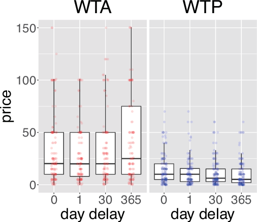
| Figure 1: Selling (WTA) and Buying (WTP) Prices across Time Scenarios
(Experiment 1). Each dot represents one observation. The horizontal line inside each box is
the median; the bottom and top of the box are the first and third
quartile, respectively. |
When discussing our results, we will focus mostly on the medians (rather
than the means), which are more robust to extreme values. All the main
patterns, however, hold in terms of means as well (see Table 1).
Consistent with previous findings on the endowment effect, the median WTA
today ($20.2) was substantially higher than the median WTP today
($10.0), and this difference was statistically significant (Mann-Whitney
test: z = 5.51, p < .01). As Figure 1 shows,
WTA was roughly constant over time, with even a small increase in the 1
year scenario, while WTP consistently decreased as the transaction was
delayed in time, resulting in an increasing endowment effect (i.e.,
WTA-WTP disparity) across time scenarios.
To further analyze these patterns, we conducted an analysis based on
quantile regressions using both conventional and clustered standard errors
(at the level of the individual)3 (Table 2). We separately regressed WTA and WTP on two
variables called Delay and Wrong. The Delay variable captures the different
time scenarios measured in days of delay, so that it takes the value 0 if
the scenario is today, 1 if it is tomorrow, 30 if it is in 1 month, and 365
if it is in 1 year. The variable Wrong is a dummy variable, taking the
value 1 if the answer to the qualification question was incorrect. The
regression results confirm that WTA did not significantly change across
time scenarios, showing even a significant increase in Regression 2 (with
clustered standard errors). On the other hand, WTP significantly decreased
as the transaction was delayed. Specifically, median WTP decreased by
around 1.3 cents per day of delay on average.
| Table 2: Quantile Regression Analysis (Experiment 1). |
| | (1) | (2) | (3) | (4) |
| | WTA | WTA | WTP | WTP |
| Delay | 0.015 | 0.015** | –0.013*** | -0.013*** |
| | (0.012) | (0.007) | (0.005) | (0.003) |
| Wrong | 5.000 | 5.000 | 0.390 | 0.390 |
| | (5.602) | (5.178) | (2.535) | (2.086) |
| Constant | 24.552*** | 24.552*** | 10.013*** | 10.013*** |
| | (2.360) | (3.099) | (0.954) | (1.502) |
| Clustered SE | No | Yes | No | Yes |
| N | 600 | 600 | 596 | 596 |
| Notes: Standard errors in parentheses; *, ** and *** stand for statistical
significance at the 10%, 5% and 1% level respectively.
|
Overall, Experiment 1 shows that the endowment effect is amplified as
transactions are moved into the future, in the form of a flat (or even
somewhat increasing) WTA across time and a consistently decreasing WTP.
3 Experiment 2: Separating the Discounting of Item and Money
In Experiment 1, both the transaction of the item and of the money happened
at the same time in the future. This resembles many real-world settings,
such as online markets, in which buyers and sellers agree on a future
moment to exchange money and item. However, this makes it difficult to
know how the temporal discounting of these two elements (item and money)
contributed to the pattern we observe. While it has been argued that
buyers do not evaluate the money paid to acquire items as a loss (Novemsky
& Kahneman, 2005), it could still be that to some extent sellers discount
the future money they will receive (which is a gain for them) more than
buyers discount the money they will pay (which is a loss for them). This
could contribute to the increasing WTA-WTP disparity we obtained in
Experiment 1. The main goal of Experiment 2 was to investigate the
endowment effect in the future, controlling for this aspect. To achieve
this, we fixed all the money transactions to take place in the present.
This also corresponds to some relevant real-world settings, such as buying
and selling with upfront payments.
3.1 Method
3.1.1 Subjects
We recruited 200 subjects (50% female, Mage =
36 years, age range: 19–86 years), who had not participated in Experiment
1, via Amazon Mechanical Turk. The study took an average of 5 minutes and
16 seconds to complete and subjects received a fixed fee of $0.5 for
their participation.
3.1.2 Design and procedure
The design and procedure used in this experiment were the same as in
Experiment 1, except that all monetary transactions were fixed to take
place in the present.
In this case, the sellers were asked “what is the minimum amount of money
($X) that you would require receiving today to sell the item and give it
up [at time t]?”; the buyers were asked “what is the maximum amount of
money ($X) that you would be willing to pay today to receive the item [at
time t]?” As in Experiment 1, the transaction timing of the item [at time
t] was today, tomorrow, in 1 month, or in 1 year, with the different time
scenarios randomized within subjects. We also used the same type of
graphical display to clarify transaction timings.
3.2 Results and discussion
Table 3 reports summary statistics for Experiment 2; Figure 2 shows the
patterns obtained in WTA and WTP across the different time
scenarios.4
| Table 3: Descriptive Statistics (Experiment 2). |
| | Time | Median | | Mean | | SD | | Total N | Wrong&outliers |
| WTA | Today | 20.0 | | 36.1 | | 41.1 | | 93 | 10 |
| | Tomorrow | 20.0 | | 31.0 | | 36.5 | | 93 | 27 |
| | 1 month | 20.0 | | 30.4 | | 31.1 | | 93 | 20 |
| | 1 year | 20.2 | | 32.4 | | 33.4 | | 93 | 26 |
| WTP | Today | 10.0 | | 13.3 | | 14.8 | | 107 | 15 |
| | Tomorrow | 10.0 | | 12.7 | | 13.5 | | 107 | 21 |
| | 1 month | 5.1 | | 9.9 | | 10.4 | | 107 | 16 |
| | 1 year | 3.5 | | 6.5 | | 9.0 | | 107 | 21 |
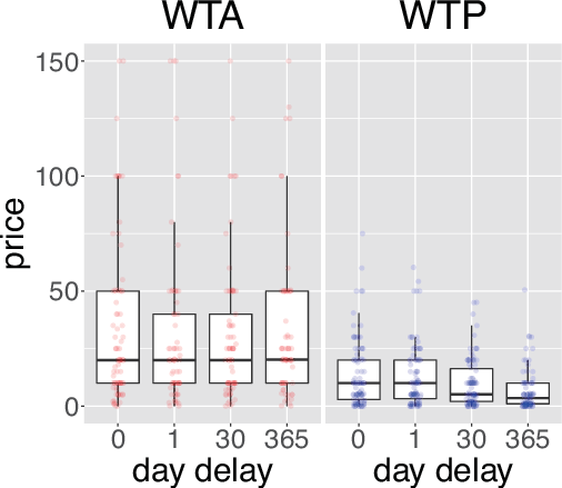
| Figure 2: Selling (WTA) and Buying (WTP) Prices across Time Scenarios
(Experiment 2). Each dot represents one observation. The horizontal line inside each box is
the median; the bottom and top of the box are the first and third
quartile, respectively. |
Again, the results were broadly in line with previous findings on the
endowment effect, namely, median WTA today ($20.0) was higher than median
WTP today ($10.0), and this difference was statistically significant
(Mann-Whitney test: z = 4.50, p < .01). As
Figure 2 shows, WTA was again roughly constant over time (in this case
without the slight increase in the 1 year scenario obtained in Experiment
1), while WTP again progressively decreased as the transaction of the item
was delayed, which resulted in an increasing endowment effect across time
scenarios. We also conducted the same quantile regression analysis as in
Experiment 1 (Table 4). The first two columns of Table 4 confirm that WTA
did not change across time scenarios. The last two columns of the table
show that WTP significantly decreased over time, by an average of 1.4
cents per day of delay (slightly more than in Experiment 1).
| Table 4: Quantile Regression Analysis (Experiment 2). |
| | (1) | (2) | (3) | (4) |
| | WTA | WTA | WTP | WTP |
| Delay | 0.000 | 0.000 | –0.014*** | –0.014*** |
| | (0.014) | (0.007) | (0.004) | (0.004) |
| Wrong | -0.500 | –0.500 | 0.014 | 0.014 |
| | (5.720) | (4.313) | (1.590) | (2.766) |
| Constant | 20.500*** | 20.500*** | 10.000*** | 10.000*** |
| | (2.667) | (4.188) | (0.675) | (1.969) |
| Clustered SE | No | Yes | No | Yes |
| N | 372 | 372 | 428 | 428 |
| Notes: Standard errors in parentheses; *, ** and *** stand for statistical
significance at the 10%, 5% and 1% level respectively.
|
As in this experiment only the item was moved in time, we can also cleanly
estimate discount factors for it based on the WTA and WTP valuations. We
have done this using the classic exponential discount function (Samuelson,
1937), D(t) = δt, where t is
the time delay to receive the relevant outcome and δ is the
discount factor. δ = 1 implies no discounting of outcomes as they
are delayed; values of δ closer to zero imply greater temporal
discounting. Including all observations, the yearly discount factor in the
seller condition was δWTA365 = 1.01; in the buyer condition,
it was δWTP365 = 0.59. This shows that in the
seller condition the value of the item was not discounted, while in the
buyer condition the item lost on average 41% of its value in one
year. Table A1 in the Appendix contains the details of these discount
factor estimations.
The results of Experiment 2 show again that the endowment effect was
consistently amplified as the transaction of the item was moved into the
future, this time controlling for the discounting of the money involved in
the transactions by fixing all monetary exchanges to take place in the
present. More specifically, WTA remained constant as the item was delayed,
but WTP progressively decreased, resulting in an increased WTA-WTP
disparity. The patterns obtained in Experiment 2 are very similar to the
ones in Experiment 1, which means that if differences between sellers and
buyers in the discounting of the money involved in the transactions play a
role, it is a very minor one. The patterns obtained seem to come primarily
from the discounting of the item.
4 Experiment 3: Robustness
across Items
In Experiments 1 and 2 we used the same item: a framed Game of Thrones
poster. This raises questions about the generalizability of the patterns
obtained and the extent to which they might depend on particular
characteristics of the item used. To test the generalizability of our
findings across items, in Experiment 3 we elicited WTA and WTP valuations
in different time scenarios for three different items, the Game of Thrones
poster (to be able to compare patterns directly) and two additional items
with markedly different characteristics.
4.1 Method
4.1.1 Subjects
We recruited 299 subjects (56% female, Mage =
37 years, age range: 20–72 years) who had not participated in Experiments
1 and 2 via Amazon Mechanical Turk. The study took an average of 9 minutes
and 52 seconds to complete and subjects received a fixed fee of $0.8
for their participation.
4.1.2 Design and procedure
The design and procedure of Experiment 3 were the same as in Experiment 2
(which was cleaner than Experiment 1 in terms of controlling for the
discounting of the money), except that the subjects evaluated three
different items instead of one. In addition to the Game of Thrones poster,
they were presented with an ordinary IKEA mug with a retail price of
€3.99, and with a hypothetical CD autographed by their favorite music
artist or band. Subjects were first asked to indicate their favorite
artist or band, and then they were told to imagine that there was a CD
autographed by them. The order of the three items was randomized within
subjects. Apart from the questions described in Experiment 1, we also
asked subjects how strongly they thought they would be emotionally
attached to each of the items if they owned them for real. The three items
were chosen because they have very different characteristics in aspects
such as link to the self, emotionality, practical value and depreciation.
In this experiment, we eliminated the tomorrow scenario to keep the number
of evaluations more manageable for subjects, so the transaction
timings were today, in 1 month and in 1 year.
4.2 Results and discussion
First of all, our results show that the three items used in the experiment
were indeed different in terms of liking, emotional attachment and
monetary valuation. The CD was liked the most, followed by the poster and
the mug (mean values: CD = 5.89, poster = 3.75, mug = 3.03; Friedman test:
Fr. = 298.84, p < .01). In terms of emotional
attachment, the CD was also rated higher, followed by poster and mug (mean
values: CD = 4.30, poster = 2.08, mug = 1.30 (Friedman test: Fr.
= 312.64, p < .01). Taking WTP in the today scenario as
a benchmark, people were also willing to pay more for the CD, followed
again by poster and mug (mean values: CD = $41.11, poster = $14.72, mug
= $4.88; Friedman test: Fr. = 181.40, p <
.01).
Table 5 reports summary statistics and Figure 3 shows boxplots like the
ones used in the previous experiments.5 The results clearly replicated the patterns obtained in
Experiment 2 across all three items. In all cases, median WTA today was
substantially higher than median WTP today, in line with the endowment
effect literature. More importantly, WTA was always essentially flat
across time scenarios, while WTP consistently decreased as the transaction
of the item was delayed, resulting in an increasing endowment effect.
| Table 5: Descriptive Statistics (Experiment 3). |
| Item | Condition | Time | Median | | Mean | | SD | | Total N | Wrong&outliers |
| Poster | WTA | Today | 20.0 | | 30.5 | | 29.7 | | 148 | 22 |
| | | 1 month | 20.0 | | 29.2 | | 27.5 | | 148 | 34 |
| | | 1 year | 20.0 | | 30.2 | | 30.1 | | 148 | 37 |
| | WTP | Today | 6.5 | | 9.6 | | 8.4 | | 151 | 23 |
| | | 1 month | 5.0 | | 7.5 | | 8.0 | | 151 | 22 |
| | | 1 year | 3.0 | | 4.3 | | 4.7 | | 151 | 22 |
| CD | WTA | Today | 75.1 | | 131.8 | | 138.0 | | 148 | 33 |
| | | 1 month | 75.0 | | 123.8 | | 141.5 | | 148 | 41 |
| | | 1 year | 75.0 | | 126.1 | | 144.5 | | 148 | 43 |
| | WTP | Today | 20.3 | | 27.9 | | 22.6 | | 151 | 15 |
| | | 1 month | 20.0 | | 22.2 | | 17.6 | | 151 | 23 |
| | | 1 year | 10.0 | | 15.3 | | 14.1 | | 151 | 27 |
| Mug | WTA | Today | 5.0 | | 5.7 | | 4.9 | | 148 | 16 |
| | | 1 month | 5.0 | | 5.8 | | 4.8 | | 148 | 22 |
| | | 1 year | 5.0 | | 5.8 | | 5.1 | | 148 | 32 |
| | WTP | Today | 3.0 | | 3.4 | | 2.7 | | 151 | 18 |
| | | 1 month | 1.7 | | 2.2 | | 2.0 | | 151 | 21 |
| | | 1 year | 1.0 | | 1.5 | | 1.8 | | 151 | 22 |
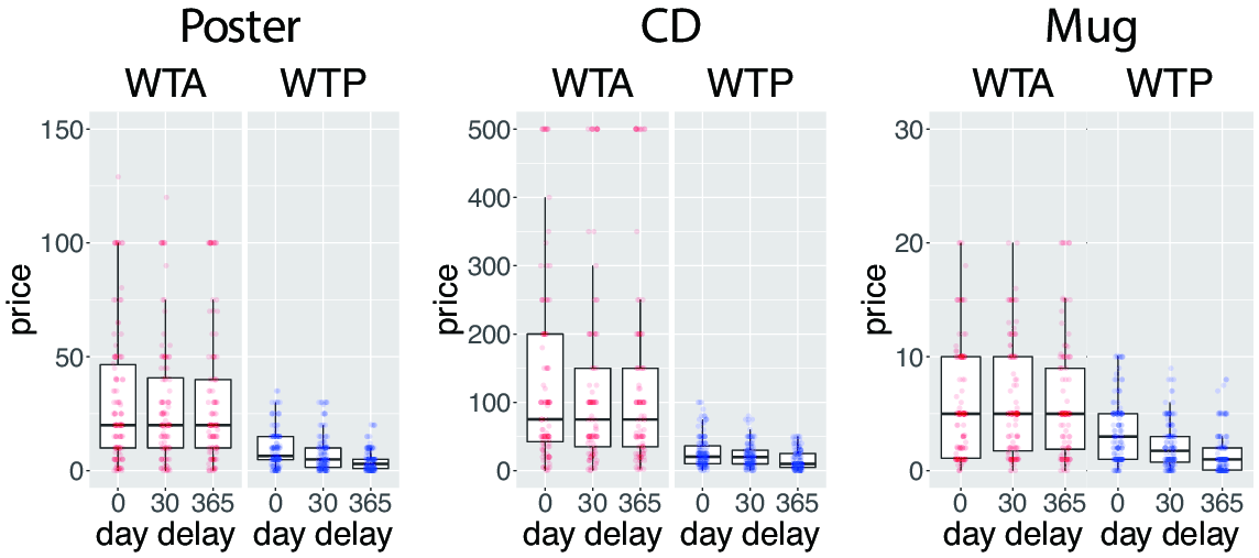
| Figure 3: Selling (WTA) and Buying (WTP) Prices of the Three Items across
Time Scenarios (Experiment 3). Each dot represents one observation. The horizontal line inside each box is
the median; the bottom and top of the box are the first and third
quartile, respectively. |
Our quantile regression analysis, summarized in Table 6 for WTA and in
Table 7 for WTP, confirms that WTA did not significantly change as the
transaction time was delayed for any of the items, while WTP significantly
decreased for all of them (by 0.6 cents per day of delay in the case of
the poster, 3 cents in the case of the CD and 0.4 cents in the case of the
mug).
| Table 6: Quantile Regression Analysis of WTA (Experiment 3) |
| | (1) | (2) | (3) | (4) | (5) | (6) |
| | Poster | Poster | CD | CD | Mug | Mug |
| Delay | –0.001 | –0.001 | 0.000 | 0.000 | 0.000 | 0.000 |
| | (0.010) | (0.005) | (0.053) | (0.027) | (0.001) | (0.001) |
| Wrong | –3.700 | –3.700 | –49.010* | –49.010** | 0.000 | 0.000 |
| | (4.719) | (4.144) | (26.023) | (21.416) | (0.686) | (1.347) |
| Constant | 20.200*** | 20.200*** | 100.000*** | 100.000*** | 5.000*** | 5.000*** |
| | (2.079) | (2.848) | (11.357) | (17.947) | (0.280) | (0.627) |
| Clustered SE | No | Yes | No | Yes | No | Yes |
| N | 444 | 444 | 444 | 444 | 444 | 444 |
| Notes: Standard errors in parentheses; *, ** and *** stand for statistical
significance at the 10%, 5% and 1% level respectively.
|
| Table 7: Quantile Regression Analysis of WTP (Experiment 3) |
| | (1) | (2) | (3) | (4) | (5) | (6) |
| | Poster | Poster | CD | CD | Mug | Mug |
| Delay | –0.006** | –0.006*** | –0.030*** | –0.030*** | –0.004*** | –0.004*** |
| | (0.003) | (0.001) | (0.006) | (0.003) | (0.001) | (0.001) |
| Wrong | –0.889 | –0.889 | 3.100 | 3.100 | 0.500 | 0.500 |
| | (1.637) | (1.509) | (3.259) | (5.451) | (0.628) | (0.648) |
| Constant | 6.189*** | 6.189*** | 20.896*** | 20.896*** | 2.500*** | 2.500*** |
| | (0.581) | (0.758) | (1.264) | (1.496) | (0.211) | (0.320) |
| Clustered SE | No | Yes | No | Yes | No | Yes |
| N | 453 | 453 | 453 | 453 | 453 | 453 |
| Notes: Standard errors in parentheses; *, ** and *** stand for statistical
significance at the 10%, 5% and 1% level respectively.
|
As in Experiment 2, we can estimate discount factors based on the WTA and
WTP valuations, which we have done using the classic exponential discount
function. Including all observations, the estimated yearly discount factors
are δWTAposter365 = 1.02, δWTAcd365 = 0.88 and
δWTAmug365 = 0.96 in the seller condition, and
δWTPposter365 = 0.56, δWTPcd365 = 0.54 and
δWTPmug365 = 0.60 in the buyer condition. This shows that
discount factors are always substantially lower (implying more discounting)
in the buyer condition. In the seller condition, the discount factors for
poster and mug imply virtually no discounting, and the factor for the CD
shows a mild degree of discounting. In the buyer condition, all discount
factors are fairly similar and they entail substantial degrees of
discounting (at least 40% of lost value with one year of delay). The
details of these discount factor estimations are in Tables A2 and A3 in the
Appendix.
Overall, Experiment 3 shows that the patterns obtained in Experiments 1 and
2 hold across different types of items. As transactions are delayed into
the future, WTA remains largely constant, while WTP substantially
decreases, resulting in an increasing endowment effect.
5 Experiment 4: Do People Anticipate the Effects of Extended
Endowment?
Experiments 1 to 3 provide converging evidence that the endowment effect is
amplified as transactions are delayed into the future, in the form of a
virtually constant WTA across transaction timings and a consistently
decreasing WTP. This suggests that people discount the value of acquiring
an item as the acquisition is delayed, which seems logical, but they do
not discount the (negative) value of giving up an item they own, or at
least not to a substantial extent.
There is, however, another possibility that can be derived from the small
literature on endowment and time. Strahilevitz and Loewenstein (1998)
showed that people’s valuation of an item they are endowed with increases
with the duration of ownership. Potentially, if people anticipate this
increase in how much they will value the item, this could push WTA
valuations up as the moment to give up the item is delayed. So, it could
be that people are actually discounting the value of giving up the item,
but this is compensated by their anticipated increase in how valuable the
item will be to them. This would not undermine the findings of Experiments
1 to 3 in any way, but it would imply a different interpretation. As
indicated in the introduction, this possibility seems unlikely, given that
a few papers have shown that people do not anticipate becoming attached to
items in endowment effect situations (Loewenstein & Adler, 1995; Van
Boven et al., 2000). However, in our setting, people are already
(hypothetically) endowed with the items and they only need to anticipate
this endowment to have a stronger effect on them as time passes, so this
possibility merits investigation.
The goal of Experiment 4 was to ask whether, in our set-up, people anticipate
becoming increasingly attached to the items and valuing them more as time
passes.
5.1 Method
5.1.1 Subjects
We recruited 201 subjects (50% female, Mage = 39
years, age range: 19–77 years) who had not participated in Experiments 1
to 3 via Amazon Mechanical Turk. The study took an average of 9 minutes
and 12 seconds to complete and subjects received a fixed fee of $0.5
for their participation. We excluded from our sample one subject who
did not meet the minimum age requirement and two subjects whose ID was
not recorded on Amazon Mechanical Turk, suggesting that they did not
register as workers on this platform.
5.1.2 Design and procedure
In this experiment, all subjects faced the same scenarios and responded
to the same questions (i.e., there was only one condition). As in the
seller conditions of the previous experiments, subjects were asked to
imagine that they had received the target item as a gift, so that they now
owned it. Then they were asked “how valuable do you think the item would
be to you [after owning it for t]?” And [after owning it for t] was either
“today”, “after owning it for 1 month” or “after owning it for 1 year”,
which are the same time delays used in Experiment 3. These questions were
answered on an 11-point scale (from 0 = not valuable at all to 10
= very valuable). Subjects responded to these scenarios for
the three items used in Experiment 3 (poster, autographed CD and mug). To
deal with potential cross-contamination issues among the different items,
subjects always evaluated the poster first, because we considered it
the most relevant item in terms of relating it to the results of all the
previous experiments. The order of CD and mug was randomized. Within each
item, the different time scenarios were also randomized.
As in the previous experiments, subjects had to answer a
qualification question before responding to each scenario. After the main
questions described above, people were also asked how much they liked the
item, how strongly they felt ownership of the item, and to complete our
demographic survey, as described in Experiment 1.
5.2 Results and discussion
Figure 4 presents box plots showing the valuations of the different items
across time scenarios.6
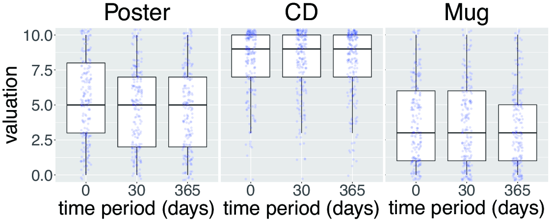
| Figure 4: Valuations of Items across Owning Periods (Experiment 4).
Each dot represents one observation. The horizontal line inside each box is
the median; the bottom and top of the box are the first and third
quartile, respectively. |
There were clear differences between the items in terms of how valuable
they were considered. The CD was perceived as more valuable than the
poster (Wilcoxon signed-rank test: z = 32.34, p
< .01), which was in turn more valuable than the mug (z
= 12.18, p < .01). This shows that subjects were
using the scale in a meaningful way. More importantly, valuations did not
change across the different owning periods. As the plots show, for all the
items, the medians were the same in the different owning periods. People
did not seem to anticipate any changes in how valuable the items would be
to them as they owned them for longer.
To further investigate this pattern, we conducted quantile regressions
using both conventional and clustered (at the individual level) standard
errors, like we did in the previous experiments (Table 8). In this case,
our dependent variable was people’s valuations of the items, and we
changed the name of our daily Delay variable used before to Period, to
reflect the fact that we are now looking at ownership periods (in terms of
days) rather than time delays. The regression results confirm that
people’s valuations did not significantly change across ownership periods
for any of the items.
| Table 8: Quantile Regression Analysis of Valuations (Experiment 4). |
| | (1) | (2) | (3) | (4) | (5) | (6) |
| | Poster | Poster | CD | CD | Mug | Mug |
| Period | 0.00 | 0.00 | 0.00 | 0.00 | 0.00 | 0.00 |
| | (0.00) | (0.00) | (0.00) | (0.00) | (0.00) | (0.00) |
| Wrong | 0.00 | 0.00 | –3.00*** | –3.00* | 2.00* | 2.00** |
| | (0.75) | (0.56) | (0.50) | (1.71) | (1.19) | (0.99) |
| Constant | 5.00*** | 5.00*** | 9.00*** | 9.00*** | 3.00*** | 3.00*** |
| | (0.23) | (0.26) | (0.12) | (0.22) | (0.30) | (0.29) |
| Clustered SE | No | Yes | No | Yes | No | Yes |
| N | 594 | 594 | 594 | 594 | 594 | 594 |
| Notes: Standard errors in parentheses; *, ** and *** stand for statistical
significance at the 10%, 5% and 1% level respectively.
|
Overall, these results show that subjects did not anticipate that the
items would be more valuable to them if they owned them for a longer
period of time, which suggests that people simply discount the value of
acquiring an item as it is delayed in time but do not discount the
(negative) value of giving it up.
6 Experiment 5:
Transactions in a Real Online Market
The experiments presented above provide evidence of endowment effects being
amplified as transactions are delayed into the future. Two limitations of
the previous experiments, however, are that the decisions are hypothetical
and they are not linked to a real-world context. In Experiment 5, we
tested the robustness of our findings in the context of a real online
market called Wallapop and with incentivized decisions. Wallapop is the
largest online flea market service in Spain, currently with more than 15
million users who have uploaded over 180 million products (according to
the Wallapop website). It is essentially a Spanish version of the American
Craigslist, where people buy and sell second-hand items and agree on a
price and a time to exchange them. This provides an ideal platform for our
study.
6.1 Method
6.1.1 Subjects
We used a web service to recruit subjects who were active Wallapop
users, defined as people who had (right before being contacted for the
experiment) a Wallapop account with at least one item on sale. They also
had to live in the city in which the authors were based and be willing to
provide the URLs of the web pages where their items were posted on
Wallapop. These URLs allowed us to check the details and history of the
items on Wallapop. Following these criteria, we recruited a sample of 130
valid subjects (48% female, Mage = 34 years,
age range: 18–72 years), who were paid a fixed fee for their participation
(managed by the recruiting company) and also had some probability of
conducting one of the transactions they were asked about for real. The
study took an average of 19 minutes to complete.
6.1.2 Design and procedure
In this experiment, we manipulated two factors within subjects: role
(seller and buyer conditions) and time scenario (transaction tomorrow and
in 1 month). The order of the role and of the time scenario was randomized
within subjects. The transaction timings were reduced to two in this
case to make the whole experiment simpler for the subjects.
In the seller condition, people were told to provide the URL of the last
active (i.e., still on sale) item they had posted on Wallapop. Then they
were asked about their WTA to sell this item for the two different time
scenarios (exchanging money and good tomorrow and in 1 month). The set-up
here is analogous to that in Experiment 1, where money and item were also
exchanged at the same time, so the specific questions used were the same
as in Experiment 1. This also mimics the typical situation found in
Wallapop, in which sellers and buyers need to agree on a future time to
exchange item and money.
In the buyer condition, subjects were asked to pick the item they liked
the most out of a selection of five different items that were on sale on
Wallapop: a smartwatch, a wireless speaker, a backpack, an electric
toothbrush, and a ukulele. These items were selected based on a pre-test
of various Wallapop items to make sure that they were on average
well-valued by people. The items were presented to the subjects in the
standard Wallapop format. Then they were asked about their WTP for the
item they had picked in the two time scenarios (exchanging money and good
tomorrow and in 1 month).
It is important to note that in this experiment WTA and WTP valuations were
elicited for different items, so they are not directly comparable. We can,
however, analyze the pattern of valuations across transaction timings
within WTA and within WTP, which is the key aspect of our findings.
As in the previous experiments, all scenarios were preceded by
qualification questions to make sure that people had understood the
instructions, and they included graphical displays to clarify transaction
timings (see Experiment 1). Subjects completed also a final survey,
asking when they had bought the item, the purchasing price, how many
buyers had contacted them about the item, the condition of the item, if
they had reposted the item on Wallapop, the reason for selling the item,
how many times they had bought items on Wallapop, and if they would be in
the city in 1 month from the day of the experiment.
6.1.3 Incentive system
In this experiment, we also incentivized people’s valuations with the
widely used Becker-DeGroot-Marschak (BDM) method (Becker et al., 1964,
described below). Several randomly selected subjects had the chance to
implement for real one of the transactions they had been asked
about. Specifically, we randomly selected three people to implement one of
their WTA valuations (also randomly selected) and two people to implement
one of their WTP valuations (also randomly selected). Subjects knew
from the beginning that they could be picked to carry out one of the
transactions, so that any one of their valuations could have real
consequences.
In the case of the selected WTA valuations, the computer then generated a
random number (from a pre-specified range). If the valuation was smaller
than or equal to this number, people were asked to sell the item to us for
the generated amount; if the valuation was higher than the number, the
item was not sold. If the item was sold, we then agreed with the selected
subject on a suitable location to exchange money and item at the
corresponding transaction time (or as close to it as possible), as is
usually done on Wallapop. These subjects were also asked to
immediately change the status of their item on Wallapop to “sale already
agreed”.
For the selected WTP valuations, the computer also generated a random
number. If the valuation was higher than or equal to the number, people
were entitled to receive the item; if the valuation was lower than the
number, people were entitled to receive an amount of money equal to the
generated number. This set-up is often used when applying the BDM method
to elicit WTP to avoid making people pay money out of their own pockets.
We then agreed with the selected subjects on a suitable location to
give them their outcome at the corresponding time (or as close as possible
to it).
6.2 Results and discussion
Table 9 reports the summary statistics for Experiment 5; the box plot in
Figure 5 shows the main patterns observed in the different
scenarios.7 The results obtained are broadly in line with Experiment 1.
Focusing on the medians, WTA slightly increased as the transaction was
delayed (i.e., in the 1 month scenario compared to the tomorrow scenario),
while WTP considerably decreased.
| Table 9: Descriptive Statistics (Experiment 5). |
| | Time | Median | | Mean | | SD | | Total N | Wrong&outliers |
| WTA | Tomorrow | 28.5 | | 62.8 | | 98.3 | | 130 | 22 |
| | 1 month | 30.0 | | 70.3 | | 113.2 | | 130 | 20 |
| WTP | Tomorrow | 20.0 | | 31.3 | | 65.8 | | 130 | 38 |
| | 1 month | 15.0 | | 20.0 | | 22.8 | | 130 | 41 |
| Figure 5: Selling (WTA) and Buying (WTP) Prices across Time Scenarios
(Experiment 5). Each dot represents one observation. The horizontal line
inside each box is the median; the bottom and top of the box are the
first and third quartile, respectively. |
As in the previous experiments, we further analyzed the results using
quantile regressions, with both conventional and clustered standard errors
(at the level of the individual) (Table 10). Given that in this case we
only had two transaction timings, we substituted the Delay variable used
in Experiments 1 to 3 with a dummy variable called 1_month, which takes
the value 1 if the transaction was in 1 month and 0 if it was tomorrow.
The regression results show that WTA was not significantly different
between the time scenarios, but WTP significantly decreased as the
transaction timing was delayed.8
| Table 10: Quantile Regression Analysis (Experiment 5). |
| | (1) | (2) | (3) | (4) |
| | WTA | WTA | WTP | WTP |
| 1_month | 1.00 | 1.00 | –5.00** | –5.00*** |
| | (6.11) | (1.73) | (2.26) | (1.34) |
| Wrong | 0.00 | 0.00 | 0.00 | 0.00 |
| | (8.30) | (7.23) | (2.47) | (2.66) |
| Constant | 26.00 | 26.00*** | 25.00*** | 25.00*** |
| | (21.68) | (7.20) | (3.64) | (3.18) |
| Clustered SE | No | Yes | No | Yes |
| N | 260 | 260 | 260 | 260 |
| Notes: Standard errors in parentheses; *, ** and *** stand for statistical
significance at the 10%, 5% and 1% level respectively.
|
The results of Experiment 5 show that the same pattern we consistently
observed in the previous experiments is also obtained in the context of a
real market, in which sellers evaluated items they already owned and were
already planning to sell, and with incentivized valuations. Again, WTA was
roughly flat across transaction timings and WTP consistently decreased,
which would result in an amplified endowment effect in the future.
7 General Discussion and
Conclusions
Our five experiments provide clear and converging evidence that endowment
effects are amplified as transactions are delayed into the future. Across
experiments, WTA remained roughly constant and WTP consistently decreased
as the transactions were delayed. Experiment 2 showed that this pattern is
not produced by the discounting of the money involved in the transactions,
but comes largely from moving the transaction of the item in time;
Experiment 3 proved that the pattern holds across diverse items;
Experiment 4 ruled out people’s anticipation of changes in value related
to owning the item as an explanation for the non-decreasing WTA; and
Experiment 5 showed that the same WTA and WTP patterns hold in the context
of a real market, with goods that were meant to be sold, and with
incentivized decisions.
Our findings in the context of goods are partially in line with the sign
effect typically observed in the context of money (Frederick et al., 2002;
Thaler, 1981). In the sign effect, both gains and losses of money are
discounted, but gains are discounted more than losses. This pattern has
also been obtained in the context of health (where it is actually
stronger) and of decisions that relate to the environment (Hardisty &
Weber, 2009). In our experiments, the value of acquiring the items is also
discounted more than the (negative) value of giving them up, but in our
case giving up the items does not seem to be discounted at all. This could
be seen as a more extreme form of sign effect in the context of goods. One
of the key differences between money and goods is that the latter can
create psychological attachment, and this can bring in psychological
mechanisms that affect WTA and how much it is discounted. We explored, and
ruled out, one such mechanism in Experiment 4, namely that people
anticipate becoming increasingly attached to the items with time. Other
potential mechanisms can be extracted from the literature on the sign
effect, although this is currently a rather small literature that has not
explored too much the psychological underpinnings of the effect.
The sign effect is sometimes explained in terms of loss aversion (Kahneman
& Tversky, 1979), which posits that losses are more impactful than gains
of the same nominal magnitude and that this difference, in turn, reduces
discounting of losses. This account is in a way just a description of the
pattern obtained. Reasoning along these lines, it seems natural that this
effect is stronger in the context of the valuation of goods, because the
psychological attachment created by goods could make the loss even more
impactful. In other words, in the context of goods, the person is not only
losing an economic asset but also the psychological connection with the
item she has created. This is consistent with our findings, in which losing
the item is virtually not discounted.
In a recent paper, Molouki et al. (2019) proposed a “contemplation-emotion”
account of the sign effect, according to which it is the more impactful
emotional experience of waiting for the outcome in the case of losses that
produces the sign effect. In the context of this explanation, our findings
also seem quite natural. The psychological attachment component of goods
is likely to make waiting for their loss more impactful than waiting for
the loss of less emotional outcomes such as money, which would result in
less discounting of the loss and a more pronounced sign effect. There is
still room to further explore the psychological mechanisms behind
different types of sign effects for money, goods and other outcomes, but
this is beyond the scope of this paper.
Finally, our findings are also of practical relevance. We live in a world
in which delayed transactions are more and more prevalent. In virtually
all forms of online buying and selling transactions are subject to some
form of delay. The rise of online platforms such as Amazon, AliExpress,
Craigslist, Facebook Marketplace, etc. has made delayed transactions one
of the most standard practices. On the one hand, this implies that
existing studies of the endowment effect (based on transactions in the
present) are likely to have underestimated the strength of the effect, at
least in relation to some real-world settings. On the other hand, our
results provide relevant guidelines on how to design market institutions.
Providing tools for buyers and sellers to exchange goods as soon as
possible, or even nudging them into doing so, might be important to
maximize agreements and minimize the market frictions associated with
endowment effects.
References
Bar-Hillel, M., & Neter, E. (1996). Why are people reluctant to exchange
lottery tickets? Journal of Personality and Social Psychology,
70(1), 17–27. https://doi.org/10.1037/0022-3514.70.1.17.
Becker, G. M., DeGroot, M. H., & Marschak, J. (1964). Measuring utility by
a single-response sequential method. Behavioral Science,
9(3). https://doi.org/10.1002/bs.3830090304.
Burson, K., Faro, D., & Rottenstreich, Y. (2013). Multiple-unit holdings
yield attenuated endowment effects. Management Science,
59(3), 545–555. https://doi.org/10.1287/mnsc.1120.1562.
Frederick, S., Loewenstein, G., & O’Donoghue, T. (2002). Time discounting
and time preference: A critical review. Journal of Economic
Literature, 40(2), 351–401.
https://doi.org/10.1257/002205102320161311.
Georgantzís, N., & Navarro-Martínez, D. (2010). Understanding the WTA-WTP
gap: Attitudes, feelings, uncertainty and personality. Journal of
Economic Psychology, 31(6), 895–907.
https://doi.org/10.1016/j.joep.2010.07.004.
Hao, L., & Naiman, D. Q. (2007). Quantile regression (Vol. 149).
Sage, London.
Hardisty, D. J., & Weber, E. U. (2009). Discounting future green: Money
versus the environment. Journal of Experimental Psychology.
General, 138(3), 329–340. https://doi.org/10.1037/a0016433.
Horowitz, J., & McConnell, K. (2002). A review of WTA/WTP studies.
Journal of Environmental Economics and Management,
44(3), 426–447. https://doi.org/10.1006/jeem.2001.1215.
Johnson, E. J., Häubl, G., & Keinan, A. (2007). Aspects of endowment: A
query theory of value construction. Journal of Experimental
Psychology. Learning, Memory, and Cognition, 33(3), 461–474.
https://doi.org/10.1037/0278-7393.33.3.461.
Kahneman, D., Knetsch, J. L., & Thaler, R. H. (1990). Experimental tests
of the endowment effect and the coase theorem. Journal of
Political Economy, 98(6), 1325–1348.
https://doi.org/10.1086/261737.
Kahneman, D., Knetsch, J. L., & Thaler, R. H. (1991). Anomalies: The
endowment effect, loss aversion, and status quo bias. Journal of
Economic Perspectives, 5(1), 193–206.
https://doi.org/10.1257/jep.5.1.193.
Kahneman, D., & Tversky, A. (1979). Prospect theory: An analysis of
decision under risk. Econometrica, 47(2), 263–291.
https://doi.org/10.2307/1914185.
Knetsch, J. L. (1989). The endowment effect and evidence of nonreversible
indifference curves. The American Economic Review,
79(5), 1277–1284. https://www.jstor.org/stable/1831454.
Loewenstein, G. (1988). Frames of mind in intertemporal choice.
Management Science, 34(2), 200–214.
https://doi.org/10.1287/mnsc.34.2.200.
Loewenstein, G. (1996). Out of control: Visceral influences on behavior.
Organizational Behavior and Human Decision Processes,
65(3), 272–292. https://doi.org/10.1006/obhd.1996.0028.
Loewenstein, G. (2000). Emotions in economic theory and economic behavior.
American Economic Review, 90(2), 426–432.
https://doi.org/10.1257/aer.90.2.426.
Loewenstein, G., & Adler, D. (1995). A bias in the prediction of tastes.
Economic Journal, 105(431), 929–937.
https://doi.org/DOI: 10.2307/2235159.
Molouki, S., Hardisty, D. J., & Caruso, E. M. (2019). The sign effect in
past and future discounting. Psychological Science,
30(12), 1674–1695. https://doi.org/10.1177/0956797619876982.
Morewedge, C. K., & Giblin, C. E. (2015). Explanations of the endowment
effect: An integrative review. Trends in Cognitive Sciences,
19(6), 339–348. https://doi.org/10.1016/j.tics.2015.04.004.
Morewedge, C. K., Shu, L. L., Gilbert, D. T., & Wilson, T. D. (2009). Bad
riddance or good rubbish? Ownership and not loss aversion causes the
endowment effect. Journal of Experimental Social Psychology,
45(4), 947–951. https://doi.org/10.1016/j.jesp.2009.05.014.
Novemsky, N., & Kahneman, D. (2005). The boundaries of loss aversion.
Journal of Marketing Research, 42(2), 119–128.
https://doi.org/10.1509/jmkr.42.2.119.62292.
Peters, E., Slovic, P., & Gregory, R. (2003). The role of affect in the
WTA/WTP disparity. Journal of Behavioral Decision Making,
16(4), 309–330. https://doi.org/10.1002/bdm.448.
Plott, C. R., & Zeiler, K. (2007). Exchange asymmetries incorrectly
interpreted as evidence of endowment effect theory and prospect theory?
American Economic Review, 97(4), 1449–1466.
https://doi.org/10.1257/aer.97.4.1449.
Reb, J., & Connolly, T. (2007). Possession, feelings of ownership, and the
endowment effect. Judgment and Decision Making, 2(2),
107–114. http://journal.sjdm.org/jdm06131.pdf.
Samuelson, P. (1937). A note on measurement of utility. Review of
Economic Studies, 4(2), 155–161. https://doi.org/10.2307/2967612.
Shu, S. B., & Peck, J. (2011). Psychological ownership and affective
reaction: Emotional attachment process variables and the endowment effect.
Journal of Consumer Psychology, 21(4), 439–452.
https://doi.org/10.1016/j.jcps.2011.01.002.
Strahilevitz, M. A., & Loewenstein, G. (1998). The effect of ownership
history on the valuation of objects. Journal of Consumer
Research, 25(3), 276–289. JSTOR. https://doi.org/10.1086/209539.
Thaler, R. (1980). Toward a positive theory of consumer choice.
Journal of Economic Behavior & Organization, 1(1),
39–60. https://doi.org/10.1016/0167-2681(80)90051-7.
Thaler, R. (1981). Some empirical evidence on dynamic inconsistency.
Economics Letters, 8(3), 201–207.
https://doi.org/10.1016/0165-1765(81)90067-7.
Tunçel, T., & Hammitt, J. (2014). A new meta-analysis on the WTP/WTA
disparity. Journal of Environmental Economics and Management,
68(1), 175–187. https://doi.org/10.1016/j.jeem.2014.06.001.
Tversky, A., & Kahneman, D. (1991). Loss aversion in riskless choice: A
reference-dependent model. The Quarterly Journal of Economics,
106(4), 1039–1061. https://doi.org/10.2307/2937956.
Van Boven, L., Dunning, D., & Loewenstein, G. (2000). Egocentric empathy
gaps between owners and buyers: Misperceptions of the endowment effect.
Journal of Personality and Social Psychology, 79(1),
66–76. https://doi.org/10.1037/0022-3514.79.1.66
Zhang, Y., & Fishbach, A. (2005). The role of anticipated emotions in the
endowment effect. Journal of Consumer Psychology, 15(4),
316–324. https://doi.org/10.1207/s15327663jcp1504_6
Appendix
Table A1: Estimation of Yearly Discount Factors (Experiment 2).
| | (1) | (2) | (3) | (4) | (5) | (6) |
| | Poster | Poster | CD | CD | Mug | Mug |
| δ365 | 1.022 | 0.962 | 0.884*** | 0.859*** | 0.957 | 0.942 |
| | (0.057) | (0.039) | (0.043) | (0.055) | (0.047) | (0.041) |
| Constant | 22.714*** | 18.682*** | 102.028*** | 73.782*** | 5.914*** | 5.267*** |
| | (0.455) | (0.257) | (1.788) | (1.630) | (0.105) | (0.078) |
| All_obs | Yes | No | Yes | No | Yes | No |
| N | 444 | 351 | 444 | 327 | 444 | 374 |
| Notes: Clustered standard errors in parentheses; *, ** and *** stand for
statistically different from 1 (i.e., from no discounting) at the 10%,
5% and 1% level respectively. These models assume an exponential
discount function (Samuelson, 1937) with a daily discount factor δ
. The variable δ365 reported is the yearly
discount factor. Columns 2 and 4 show results excluding observations one
standard deviation above the mean and with wrong answers in the
qualification questions. All regressions include individual fixed effects.
|
Table A2: Estimation of Yearly Discount Factors for WTA (Experiment 3).
| | (1) | (2) | (3) | (4) | (5) | (6) |
| | Poster | Poster | CD | CD | Mug | Mug |
| δ365 | 1.022 | 0.962 | 0.884*** | 0.859*** | 0.957 | 0.942 |
| | (0.057) | (0.039) | (0.043) | (0.055) | (0.047) | (0.041) |
| Constant | 22.714*** | 18.682*** | 102.028*** | 73.782*** | 5.914*** | 5.267*** |
| | (0.455) | (0.257) | (1.788) | (1.630) | (0.105) | (0.078) |
| All_obs | Yes | No | Yes | No | Yes | No |
| N | 444 | 351 | 444 | 327 | 444 | 374 |
| Notes: Clustered standard errors in parentheses; *, ** and *** stand for
statistically different from 1 (i.e., from no discounting) at the 10%,
5% and 1% level respectively. These models assume an exponential
discount function with a daily discount factor δ . The variable
δ365 reported is the yearly discount factor.
Columns 2, 4 and 6 show results excluding observations one standard
deviation above the mean and with wrong answers in the qualification
questions. All regressions include individual fixed effects.
|
Table A3: Estimation of Yearly Discount Factors for WTP (Experiment 3).
| | (1) | (2) | (3) | (4) | (5) | (6) |
| | Poster | Poster | CD | CD | Mug | Mug |
| δ365 | 0.558*** | 0.536*** | 0.542*** | 0.508*** | 0.603*** | 0.591*** |
| | (0.025) | (0.028) | (0.033) | (0.035) | (0.022) | (0.024) |
| Constant | 7.863*** | 6.612*** | 21.499*** | 19.600*** | 3.754*** | 3.279*** |
| | (0.129) | (0.126) | (0.477) | (0.467) | (0.050) | (0.047) |
| All_obs | Yes | No | Yes | No | Yes | No |
| N | 453 | 386 | 453 | 388 | 453 | 392 |
| Notes: Clustered standard errors in parentheses; *, ** and *** stand for
statistically different from 1 (i.e., from no discounting) at the 10%,
5% and 1% level respectively. These models assume an exponential
discount function with a daily discount factor δ . The variable
δ365 reported is the yearly discount factor.
Columns 2, 4 and 6 show results excluding observations one standard
deviation above the mean and with wrong answers in the qualification
questions. All regressions include individual fixed effects.
|
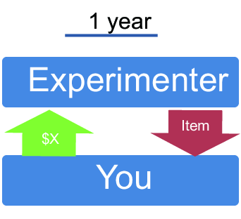 Figure A1
. Graphical Display used to Clarify Transaction Timing (Buyer
Condition, 1 Year Scenario).
This document was translated from LATEX by
HEVEA.