| Figure 1: Human-machines process control framework. |
Judgment and Decision Making, Vol. 17, No. 3, May 2022, pp. 598-627
Combining white box models, black box machines and human interventions for interpretable decision strategiesGregory Gadzinski* Alessio Castello# |
Abstract: Granting a short-term loan is a critical decision. A great deal of research has concerned the prediction of credit default, notably through Machine Learning (ML) algorithms. However, given that their black-box nature has sometimes led to unwanted outcomes, comprehensibility in ML guided decision-making strategies has become more important. In many domains, transparency and accountability are no longer optional. In this article, instead of opposing white-box against black-box models, we use a multi-step procedure that combines the Fast and Frugal Tree (FFT) methodology of Martignon et al. (2005) and Phillips et al. (2017) with the extraction of post-hoc explainable information from ensemble ML models. New interpretable models are then built thanks to the inclusion of explainable ML outputs chosen by human intervention. Our methodology improves significantly the accuracy of the FFT predictions while preserving their explainable nature. We apply our approach to a dataset of short-term loans granted to borrowers in the UK, and show how complex machine learning can challenge simpler machines and help decision makers.
Keywords: fast and frugal trees, ensemble neural networks, Bayesian uncertainty, partial dependence plots
“Machines can decide, but only humans can choose!”, Garry Kasparov.
Short-term loans provide an important financial opportunity for consumers. In a recent study, Deku et al. (2016), using information from almost 60.000 households in the UK, observed that barriers to essential financial services such as short-term loans can hinder both economic and social development. The most common method used by lending institutions and banks to decide whether to grant a loan uses credit scores: Credit Reference Agencies collect historical financial data of consumers and sell them to lending institutions that apply in-house developed algorithms to calculate an aggregate score. A cutoff model in then used according to which all loan applicants with a score above a certain threshold are granted the requested amount, while those with a score inferior to the threshold are denied the loan.
The accuracy of the estimation of clients’ probability of default is pivotal to the success of lending institutions; indeed a minor change in the model can yield a marginal improvement in the absolute performance, which eventually lead to a significant impact on the business profits and savings (Crook, Edelman & Thomas, 2007; Derelioğlu & Gürgen, 2011). This is the reason why a considerable number of techniques has been deployed to achieve higher accuracy (Fu, Huang & Singh, 2021). Non parametric Machine Learning techniques have been in use for decades (Harris, 2015; Lessmann, Baesens, Seow & Thomas, 2015) and, more recently, ensemble strategies have been adopted by combining the decisions of multiple classifiers to deliver a final aggregate output (Florez-Lopez & Ramon-Jeronimo, 2015). Ensemble methods trained from different initializations and/or different sets of the training data have also been used for the computation of the variance of the predictions, and then interpreted as its predictive uncertainty (Gadzinski & Castello, 2020).
Besides accuracy, the comprehensibility of the model is essential in loan applications: increasingly lending institutions are required (by regulation) to justify their denial of a credit (Hand, 2006; Tomczak & Zięba, 2015). Comprehensibility has different meanings, ranging from explainability, i.e. the ability to explain a prediction in understandable terms; to interpretability: the possibility to explain the whole model and the set of rules governing it. The call for interpretability in decision strategies guided by Machine Learning (ML), especially in contexts of high societal and human sensitivity, is getting more important (Rudin, 2019): access to finance is, among others, an area in which the lack of interpretability or, at least, explainability of predictive models can have severe consequences. If ML based models have become more accurate, their non-interpretable nature (black-box) has led to harm, or the suspicion of harm, resulting from unwanted outcomes (Varshney & Alemzadeh, 2017) or biases (Fu et al., 2021). A gap has thus emerged between the research in credit scoring that pushed accuracy to the limit, and practice-oriented needs that required interpretable models (white-box) (Finlay, 2011).
However, accuracy and comprehensibility are two features that need to be balanced, i.e., an optimal equilibrium is required in the accuracy-interpretability trade-off (Chen & Cheng, 2013; Hayashi & Takano, 2020). Having said that, the number of ML models that are both more accurate and interpretable has been rising recently, with a large strand of the literature on artificial intelligence now focusing on explainability (Ribeiro, Singh & Guestrin, 2016).
Post-hoc information can be extracted from any ML models, using for example popular approaches such as Partial Dependence Plots (PDP) and Accumulated Local Effects (ALE) (Apley & Zhu, 2020; Greenwell, 2017). Yet, since it can be challenging to understand the complex relationships that a model has learned, the presentation of the results becomes particularly important.
Our research aims at developing innovative combinations of existing tools with the intention to help increase the accuracy of interpretable models. To achieve our goals, we have developed a number of different visualization tools that assess both the main effects of the individual predictor variables and their low-order interaction effects. Instead of comparing white-box and black-box models (Olson, Delen & Meng, 2012), we combine them; and therefore, by doing so, we address the issue of balancing interpretability and accuracy. Moreover, our multi-step sequential methodology procedure is also an application of human-machines interactions in the quest of better performance, following the work of Licklider on “man-computer symbiosis” (Licklider, 1960). Thus, we propose a decision-making framework for building augmented interpretable models, using human-computer collaboration, in line with the concept of interpretable Decision Support System (iDSS) introduced by Coussement et al. (2021). We apply our procedure to a dataset of short-term loans granted to borrowers in the UK and test the performance of several competing models.
Our research refers to several streams of academic investigation, we report in the following the key findings in the various fields of relevance.
Scholars have identified a certain ambiguity between the terms explainability and interpretability (Krishnan, 2020). In the remainder of this article, we adopt the following definitions: Interpretability is the ability to demonstrate and understand the internal workings of the model, i.e. how the model uses input features to make predictions (Barredo Arrieta et al., 2020; Kraus & Feuerriegel, 2019; Lakshminarayanan, Pritzel & Blundell, 2017; Pintelas, Livieris & Pintelas, 2020). This may include understanding decision rules and cutoffs, and the ability to manually derive the outputs of the model, e.g., if the loan applicant has more than 10 years of experience within the same company, the loan is granted.
Explainability refers to a mechanism that provides to humans (partial) information about the workings of the model, such as identifying influential features, highlighting potential relationships — such as the existence of a negative relationship between years of experience and probability of defaulting on a loan — but without any structural guarantee.
The spectrum of interpretability ranges from heuristics (educated guess, trial and error, take the best,…) and standard decision trees, considered as the most interpretable ones, to neural networks as the least explainable. Heuristics of particular interest are Fast and frugal trees (FFT) (Martignon et al., 2005), in which variables are clearly identified and considered individually in a sequential way. FFT are especially suitable for binary types of decisions, e.g. should a certain client be extended the requested loan.
In terms of interpretability, linear regressions come next: clearly identified independent variables are given a specific weight and contribute to predicting the outcome.
The least interpretable decision strategies include ML based predictive models that are used in a growing set of applications including high stakes domains such as criminal justice, public policies, healthcare, access to finance and education (Burrell, 2016; Cabitza, Rasoini & Gensini, 2017; Luo et al., 2019; Rudin, 2019; Waa, Schoonderwoerd, Diggelen & Neerincx, 2020). Many current ML methods, such as neural networks (NN) and random forests are black boxes: their predictive behavior is highly accurate, but also too complex to be understandable, including to domain experts (Jang, 2019; Pintelas et al., 2020; Subramania & Khare, 2011). Being able to understand and explain decisions based on ML systems is thus a priority for data scientists and practitioners.
Rudin (2019) highlights the problems associated with using explainable systems — “explanations are often not reliable, and can be misleading” — and urges data scientists to use interpretable models instead. Indeed, a different approach to post-hoc explanations of black-box models consists in building interpretable models, which provide their own explanations, and are faithful to what the model actually computes (Kraus & Feuerriegel, 2019; Rudin, 2019). Interpretable models can be explained in their entirety in understandable terms to a human as opposed to reverse engineering single decision outcomes. Interpretability also offers a number of side benefits since it can be used to confirm other important features such as fairness, unbiasedness, non-discrimination, privacy, reliability and robustness, causality, usability and trustworthiness (Dwork, Hardt, Pitassi, Reingold & Zemel, 2012; Gilpin et al., 2018; Hardt & Talwar, 2010; Topuz & Delen, 2021). It also allows to overcome the natural distrust of humans towards automated predictive models (Dietvorst, Simmons & Massey, 2015; Shin, 2020, 2021d), and determines whether humans are able to reap the full benefits of ML or not (Jussupow, Spohrer, Heinzl & Gawlitza, 2021). A quite interesting illustration of human-machine trust building processes is provided by the work of Donghee Shin who studied extensively the interaction between humans and chatboxes (Shin, 2021c, 2022); among the key findings, the author mentions that causability and explainability play a dual role in affecting trustworthiness and user behaviors (Shin, 2021a, 2021b).
In order to achieve interpretability, scholars have underlined the importance of starting from simple, interpretable decision strategies and enrich them with more accurate processes only if needed (Kraus & Feuerriegel, 2019). Interpretable models require sparsity (Bertsimas, King & Mazumder, 2016): since humans can apparently process simultaneously no more than three to seven cognitive entities, sparsity becomes an essential feature of interpretability (Cowan, 2010; Miller, 1956). The analogue of sparsity when using classification trees is a small number of nodes (Bertsimas & Dunn, 2017), an example of which are heuristics and more specifically Fast and Frugal Trees — FFT — (Martignon et al., 2005).
Recently, to cope with the growing demand for more accuracy, professionals have developed tools to help data scientists and practitioners understand better how machine learning works. In other words, tools exist to help users providing post-hoc explanations for the predictions made by complex models; examples are, among others, the Local Interpretable Model-agnostic Explanations – LIME – (Ribeiro et al., 2016), the Shapely Additive expPlanations – SHAP – (Lundberg & Lee, 2017), and more recently the Local Interpretation-Driven Abstract Bayesian Network-LINDA-BN (Moreira et al., 2021). The flexibility embedded in those methods allows working with any ML model, such as random forests or deep neural networks. Once the information has been extracted from the fitted model, it can be analyzed using exploratory data analysis techniques. Other popular approaches are the Partial Dependence Plots (PDP) and Accumulated Local Effects (ALE). They are prediction-level interpretation methods that focus on explaining the average influence that features and/or interactions have on the model’s prediction (Apley & Zhu, 2020; Greenwell, 2017). Thus, they may highlight more complexity between variables with possibly non-monotonic or non-linear features undetected by simpler models.
Another prerequisite for trustworthy decisions is stability: when models attempt to answer scientific questions, notably when there is a large downside to incorrect predictions, they must be robust to reasonable perturbations (Murdoch, Singh, Kumbier, Abbasi-Asl & Yu, 2019). Unfortunately, many models are generally not immune to instability with respect to small perturbations of the training data. Consequently, an aspect often neglected in the literature is the uncertainty surrounding the estimation of interpretable models. Ensemble methods have long provided a simple way to estimate uncertainty: they aggregate the estimates of multiple baseline models, trained from various initial parameters and/or noisy versions of the training data (Lakshminarayanan et al., 2017). The ensemble’s predictions is then used to gauge the uncertainty surrounding the model predictions. Pearce et al. (2020) proposed a modification to the usual ensembling methodology by incorporating Bayesian behaviors. Their randomized Maximum-A-Posteriori (MAP) sampling estimators, combined with prior estimates, as commonly used in Bayesian methods, achieve a high degree of uncertainty accuracy.
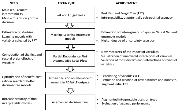
In this article, we suggest and test a new decision strategy that integrates the considerations described above: starting from simple, interpretable models, we enrich them with ML explainable outputs, and then quantify the uncertainty surrounding these predictions using ensemble methods. To do so, we also make use of human-machines collaboration (Licklider, 1960). A fundamental assumption behind human-computer symbiosis is that computers and humans have different problem-solving capabilities, and their combination yields better performance. We highlight our procedure in the process control framework depicted in Figure 1.
Figure 1: Human-machines process control framework.
Here, instead of comparing white-box and black-box models (Olson et al., 2012), we combine them; and therefore, by doing so, we address the issue of balancing interpretability and accuracy. As shown in Figure 1, we start from Fast and Frugal Trees that ensure interpretability thanks to their sparsity and simplicity. Then, we deploy Machine Learning ensemble models, limited to the variables selected by our FFT, to both reassess the dynamics between dependent and independent variables, and estimate accurately the uncertainty of the impact of each variable. In order to visualize the marginal effect that a feature has on the predicted outcome of the ML models, we use Partial Dependent Plots and Accumulated Local Effects. We then investigate the magnitude of the interaction of dyads of variables and represent them using bi-dimensional Partial Dependence Plots: among the assumptions behind the use of decision trees is the presumed independence between variables; yet, second order effects may and often do exist. Our methodology allows the selection of the most significant interactions between variables and their graphical representation. At this stage, based on the interpretation of the plots obtained, we can first decide if a reshuffling of the order in which the variables are analyzed in the FFT could yield better performance. Moreover, we may choose which new branches should be added to the initial decision tree in order to make it more accurate. To ensure interpretability and ease of execution, we allow for a maximum of one additional branch per node.
The spectrum of interpretable methods ranges from simple heuristics and decision trees, where information is deliberately truncated, to linear regressions where all the variables as well as their relationships are clearly identified and given a specific weight. Parpart et al. (2018) argue that heuristics are extreme variations of Bayesian learning models and outperform more complex models only when the heuristic specification is close enough to the data generating process. Brighton et al. (2015) have stressed that under an environment of high uncertainty (i.e. where little is known about causal processes and observations are sparse), simpler methods are generally less prone to instability, thus turning the bias-variance trade-off in their favor.
One of the most succinct forms of decision trees is the Fast-and-Frugal Tree (FFT) (Martignon, Katsikopoulos & Woike, 2008; Martignon et al., 2005). FFTs impose restrictions on the size and shape of the selected trees by having an exit branch at every node; consequently, they make decisions faster on average than standard trees.
Figure 2 shows a FFT restricted to have only 2 nodes and illustrates how it classifies individuals as being solvent or not. The first node selected by the FFT corresponds to the seniority of the loan applicant in her current job. The FFT implies that if the applicant has occupied the current position for 5 years or less, the loan should not be granted; if it is higher than 5 years, a decision cannot be reached and we move on to assess the next node. The second cue refers to the historical record of default: if the loan applicant has ever defaulted, the loan is not granted, otherwise the FFT classifies it as good borrower.
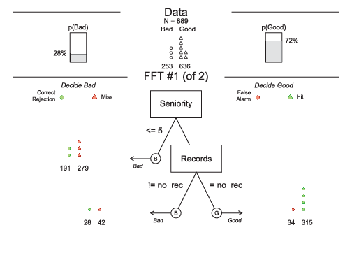
Figure 2: Visualization of a restricted FFT object with two variables (Phillips et al., 2017). The top panel shows the frequencies of negative and positive criterion classes. The middle panel contains the FFT with icon arrays displaying the accuracy of cases classified at each node.
When the algorithm chooses the most significant variables, i.e., ranks the cues and optimize their thresholds, it does so by maximizing a statistic that is related to accuracy. For instance, one can balance sensitivity (percentage of cases with correct hit rates) and specificity (percentage of cases rejecting false alarms), the so-called weighted accuracy, which in turn influences the well-known confusion matrix (Figure 3).
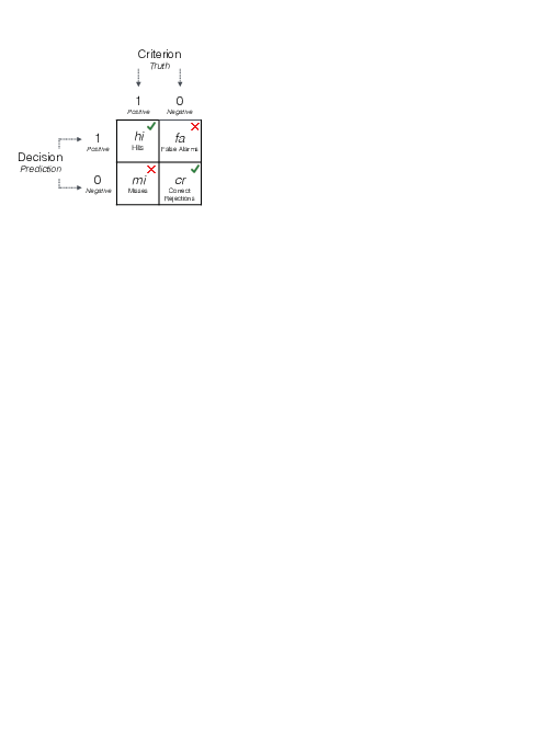
Figure 3: A 2x2 confusion matrix used to evaluate a decision algorithm from Phillips et al. (2017).
Formally,
| sensitivity = |
| (1) |
| specificity = |
| (2) |
| Accuracy = |
| (3) |
| weighted accuracy (wacc) = w · sensitivity + (1−w) · specificity (4) |
Where w is a parameter between 0 and 1 that specifies how sensitivity is weighed relative to specificity.
Although overall accuracy is an important measure, it can be misleading; in the case of imbalanced datasets, algorithms can have a high overall accuracy without being very useful when they do not distinguish between positive and negative cases. In decision tasks where sensitivity is more important than specificity (like granting a loan to an insolvent borrower), wacc could be calculated with a value of w larger than 0.5. In cases where both measures are deemed equally important, the sensitivity weight is simply set to 0.5; the so-called bacc.
In this article, we use the FFTrees toolbox written in the R Language by Phillips et al. (2017) and choose their ifan optimization algorithm as our benchmark. As explained by the authors, the ifan optimization algorithm assumes independence between cues and uses a brute-force method to optimize the decision thresholds and directions for each cue, ranking them from the most significant to the least significant (Phillips et al., 2017). After creating a set of several trees with different exit structures, these trees are then pruned to remove non-discriminant nodes; the tree with the highest accuracy measure is finally selected. Figure 4 describes the different steps of the algorithm with the use of the bacc measure (for more details, the reader should refer to the original article).
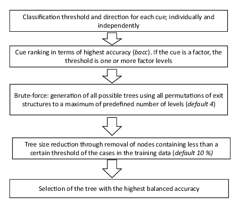
Figure 4: ifan algorithm, adapted from Phillips et al. (2017).
The purpose of this section is to explain how we use machine learning and notably neural networks to reassess the links between the explanatory variables and the dependent variable: the loan default. In the realm of classification predictions, recent studies have shown that ensemble learning methods generally outperform individual classifiers in modelling credit risk (Lessmann et al., 2015; Papouskova & Hajek, 2019). While there is nowadays a wide range of schemes available to researchers, ensembles of classifiers follow the same general principle: they imply training a set of individual (base) models for the same task, and then combine their decisions following pre-defined criteria. The ensemble superior performance is a direct consequence of the bias-variance trade-off: a combination of forecasts, i.e. adding complexity, implies a smaller error variance than any of the individual methods if base classifiers are both accurate enough and diverse. Incidentally, one can use the error variance of the ensemble to estimate uncertainty. Diversity in ensembles can be achieved in different ways, by averaging over bagged (Random Forest), boosted (Extreme Gradient Boosting or XGBoost) or randomized multiple models (Lakshminarayanan et al., 2017).
Recently, Bayesian inference has attracted much attention despite earlier evidence that it did not produce enough diversity (Sun, Li, Huang & He, 2014). The estimation of the distribution as opposed to a point estimate became state-of-the-art for estimating the so-called predictive uncertainty (Gal & Ghahramani, 2016). More recently, Pearce et al. (2020) uses a Maximum-A-Posteriori (MAP) estimator combined with appropriate priors, as commonly used in Bayesian methods, and argue that they achieve a high degree of uncertainty accuracy. The authors refer to this family of procedures as randomized MAP sampling. We now give some details on this methodology.
Starting from the maximization of the posterior density:
| θMAP(x)=argmaxθ f(θ ,x) (5) |
where θ is a vector of NN parameters
The loss function defined by Pearce et al. (2020) during the NN training is proportional to the negative log likelihood with a L2 regularization penalty added to prevent overfitting.
Thus, for classification, cross-entropy is minimized using the following loss function:
| Lossclass,j= |
|
|
| logyn,c+ |
| ∥ Γ |
| * (θ j−θ 0,j)∥22 (6) |
where yc is the class label for our two classes (default, non-default), and Γ is a diagonal square matrix. The subscript j represents one instance of the ensemble of M neural networks, with 1 ≤ j ≤ M.
However, customized losses can be also implemented, notably to mirror the FFT analysis, so that one can use a loss function that combines specificity and sensitivity.
| Lossclass,j=1−( w * sensitivity + (1−w) * specificity ) + |
| ∥ Γ |
| * (θ j−θ0,j)∥ 22 (7) |
The parameters minimizing the loss function can be interpreted from a Bayesian perspective as randomized maximum-a-posteriori (MAP) estimates with a normal prior. The challenge comes in setting the anchor noise distribution, θ0,j ∼ N(µ0,Σ0). It is interesting to note that the first term in equations (6) and (7) pulls solutions toward the likelihood distribution, whilst the second term anchors them to their prior draw. Hence, the relative strength of each is managed by the regularization matrix, which must be then fine-tuned in order to provide enough diversity while preserving some notion of prior. Notably, the prior variance-covariance matrix Σ0 is key in defining the amount of certainty present in the NNs. The higher the predictive variances, the higher the diversity. No studies have been conducted on the optimization of those parameters. Thus, for consistency, the variances of the neural network parameters are set equal to the variance of the dependent variable. We use the following network architecture: 2-hidden layers NN containing 64 hidden units with ReLU and sigmoid nonlinearities, estimated 10 times with randomly distributed anchored parameters1.
As stated above, explainable machine learning refers to a post-hoc explanation of a predicted output whereby the predictions are made without implicitly knowing the mechanisms behind which the models work. Nonetheless, these approximations remain useful in assessing if one should trust a prediction and/or identify why a feature should not be used.
Examples of such post-hoc interpretations are Partial Dependence Plots (PDP) and Accumulated Local Effects (ALE). A PDP plot shows the marginal effect that one feature has on the predicted outcome of a ML model (Greenwell, 2017). Like simple regression models, which average over the excluded explanatory variables, partial dependence works by averaging the ML output over the marginal distribution of all the features in a given set L. By using the marginal probability density, the partial dependence function provides a description of the nature of the variation of the predicted output for a chosen value(s) of a feature. As defined by Friedman (2001):
| fl, PDP(xl)= Ex ∖ l f(x) = | ∫ | f(xl, x ∖ l)p ∖ l(x∖ l)dx∖ l (8) |
Where xl denote the subset of predictors excluding xl, and where pl(xl) denotes the marginal distribution of xl.
Thus, a PD plot is the plot of the ‘main effects’ dependence fl,PDP(xl) on the fitted model f(xl, x ∖ l)
The crucial point in a Partial Dependence model is that its computation requires extrapolation beyond the envelope of the training data. This is both time consuming and may be highly inaccurate when there are none or few data points or/and when the variables are highly correlated. To cope with the lack of precision resulting from the extrapolation, one may use conditional density instead of the marginal density. However, the so-called Marginal Plots still suffer from the omitted variable bias problem because they ignore (marginalize) the other features, leading to the inclusion of both direct and indirect effects.
In a nutshell, as long as the assumption of independence between the features is valid, PDP and Marginal Plots are reliable indicators of the effect of X’s on Y. However, if the independent variables are correlated, both methods suffer from their own biases and then become unreliable indicators. To alleviate this shortcoming, Apley et al. (2019) proposed the so-called Accumulated Local Effects (ALE). The authors use the following function:
| ĝj,ALE(xj)= | ∫ |
| E fj(xj, x∖ j)| xj= zj dzj (9) |
Where
| fj(xj, x∖ j)= |
| (10) |
represents the local effect of xj on f (.) at (zj,xj), calculated as the weighted average across all values in xj with weights given by the conditional density instead of the marginal density, in order to avoid the extrapolation that is required in PD plots. In equation (9), the accumulation of the partial derivative over the local range of features (from xmin,j to xj) gives the underlying global effect of the feature on the prediction. The use of the derivative isolates the effect of the feature of interest and thus removes the effect of correlated features. For the actual computation, a grid of local intervals over which one computes the paired differences in the prediction is used. Hence, equation (9) represents the changes in the function f (.) as the variable x changes from the lower bound of the local interval to its upper bound.
Finally, the centered ALE main effect is then defined as:
| fj,ALE(xj)= ĝj,ALE(xj)− | ∫ | gj,ALE(zj) pj(zj)dzj (11) |
Equation (11) centered the ALE on zero, hence the function can be interpreted as the global partial effect of the feature (at a certain value) compared to the average prediction.
In order to assess the validity of our approach, we apply it to a dataset of short-term loans granted to borrowers in the UK over several years until 2020. The processes of estimation and visualization can be generalized to any datasets. The information we have concerns 4445 loans granted to individual customers who had no previous records with the lending organization. Access to these data was granted by a senior executive in the industry; our collaboration is governed by a Non Disclosure Agreement, under which we can only share the results of the various statistical analyses performed.
To describe each loan, we have a set of 13 independent variables (see Table A1 in the Appendix), which include both demographic descriptors (employment, age, etc.) and economic information (income, assets, debts, etc.). The dataset also includes one dependent binary variable recording the default on the loan.
In the remaining of this section, we apply the methodology described in the Methodology section to the dataset of short-term loans.
The dataset was divided into two subsets: a training set (80% of observations) for finding the optimal parameters, and an independent test set (20% of observations), displayed in the following figures. We apply the ifan algorithm of the standard Fast and Frugal Tree developed by Phillips et al. (2017). Figure 5 displays the tree with the best “balanced accuracy” (bacc), i.e. the trade-off between sensitivity (percentage of cases with correct hit rates) and specificity (percentage of cases rejecting false alarms).
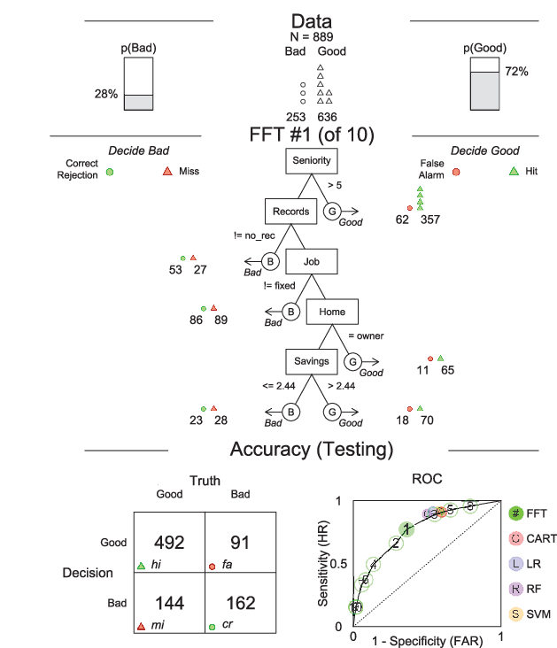
Figure 5: Visualization of an FFT with five variables (Phillips et al., 2017). The top panel shows the frequencies of negative and positive criterion classes. The middle panel contains the FFT with icon arrays displaying the accuracy of cases classified at each node. The bottom panel shows the confusion matrix, and the FFT’s ROC classification performance.
The overall accuracy statistics in the testing data are visible in the bottom panel from both the confusion matrix and the Receiver Operating Characteristic (ROC) curve. The ROC curve illustrates the trade-off between sensitivity (sens) and specificity (spec) of different algorithms, namely, 10 models coming from the FFT as well as 5 other competing models: the standard decision tree (CART), using the rpart package (Breiman, Friedman, Olshen & Stone, 2017); the logistic regression (LR), using the stats package (Phillips et al., 2017); the L2 regularized regression (RLR), using the glmnet package (J. Friedman, Hastie & Tibshirani, 2010); the random forest algorithm (RF), using the random Forest package (Breiman, 2001); and the Support Vector Machine (SVM) algorithm, using the default methodology in Karatzoglou et al. (2006). The numbers represent the rank order of the FFT algorithms performance in terms of their wacc values.
The best tree (the one maximizing the bacc) selects only five cues (out of a maximum of six allowed by the algorithm) defining for each leaf, a threshold and a decision, finally divided between good hits and false alarms. For instance, the first cue refers to the seniority of the loan applicant in her current job. The FFT implies that if the applicant has occupied the current position for five years or more, the loan should be granted. The testing data show that out of the 404 applicants with more than 5-year seniority, 354 paid back the loan and 50 defaulted. However, some nodes and decisions are more inconclusive. For instance, the third node that classifies a remaining application with no fixed job as “Bad”, gives rather weak results as it manages to capture barely more than 50% of defaulted loans. Having said that, if the FFT is aimed at maximizing the bacc measure (73%), we must note that it also performs relatively well in terms of overall accuracy (see Equation (3)), achieving similar testing results (acc: 74%) compared to the competing FFT model which maximizes overall accuracy (testing results acc: 74%)2.
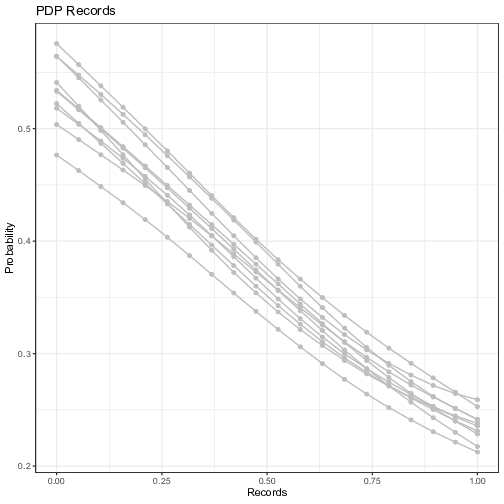
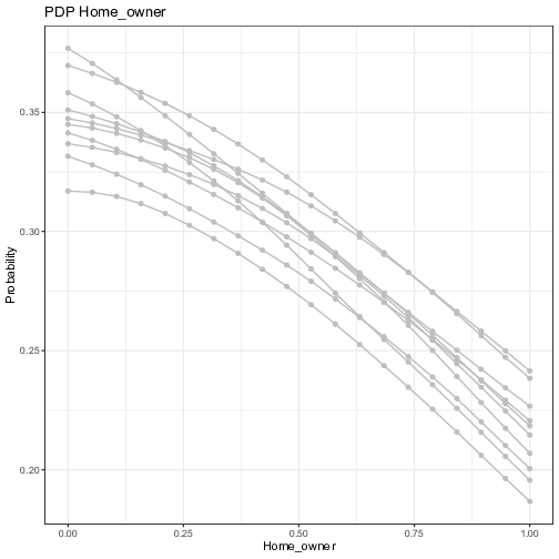
In order to assess the selection of features and the corresponding thresholds found by the best performing tree, we now move to visualizing the main effect of the individual predictor variables and their low-order interaction effects thanks to the ensemble of NNs and the Partial Dependence Plots as described previously. As stated above, for classification, whereas the ML model outputs probabilities, the Partial Dependence Plot displays the average prediction for the probability of default given the different values of each feature. We run the ensemble of 10 independent NNs with different initialization parameters, and compute the PDP for each trained model. The influences of the five features selected by the FFT on the probability of default is visualized in Figure 6.
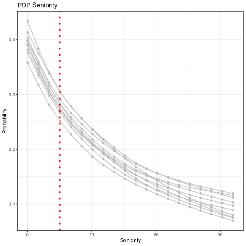
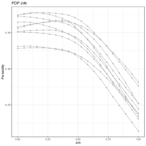
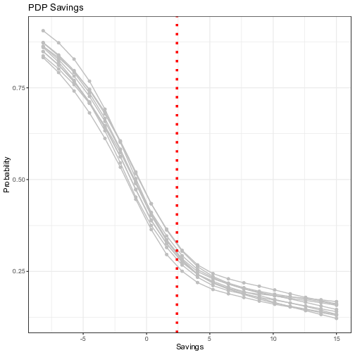
Figure 6: Visualization of the ensemble first-order Partial Dependence Plots. Each line represents the partial dependence function of one trained neural network model. The y-axis represents the average prediction of the probability of default (1 = default) and the x-axis represents the values of the original independent variables. For the continuous variables, the vertical line in red represents the threshold computed by the FFT in Figure 5.
Overall, the results are in line with those of the FFT, with the predicted probability of default decreasing with variables turning more positive. The variable “Seniority” shows the highest impact with the probability of default becoming as low as 10% for value of “Seniority” beyond 30 years. The predicted probability decreases (only) by 1/3 when one goes from zero to five years of experience, which makes the threshold given by the tree a “bold” choice. Indeed, one will need to have 10 years of experience to decrease the same probability by half compared to “no experience”. One must notice that there is little uncertainty surrounding the estimates of the impact though. More uncertainty revolves around the other variables, notably for the variables “Home” and “Job”. For instance, the probability of defaulting does not go down significantly with the presence of a “fixed” job, which is in line with the inconclusive results of the FFT testing sample in Figure 5. For the variable “Savings”, the probability of default, starting from a high level for low rates (as high as 85%), decreases sharply and takes acceptable levels (below 37.5% for positive savings), before the threshold given by the tree is reached. This last result can explain why the tree, which classifies consumers below this threshold as “Bad”, misses on many non-defaulters.
As we have seen, the Partial Dependence Plots help us to achieve a finer analysis by showing how the average prediction of the probability of default changes when a feature is changed. If the feature for which we computed the PDP is not correlated with other features, assuming sufficient data, then the PDP represents its influence. However, if the assumption of no correlation is violated, the averages calculated by the PDP will most likely include data points that are very unlikely to happen in reality. One can imagine that some features in our dataset are correlated, and that therefore, the Accumulated Local Effects (ALE) may be better at capturing whether W, X or Z is significantly relevant.
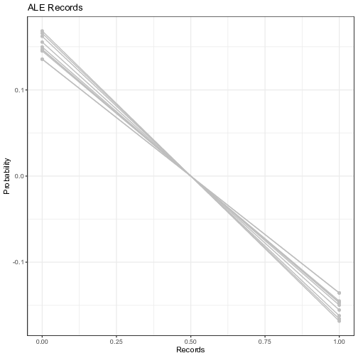
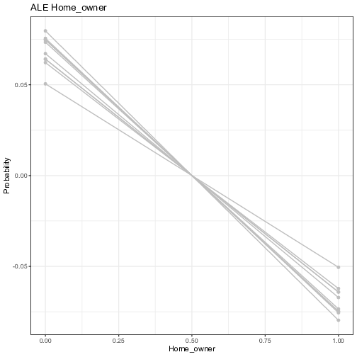
Figure 7 plots the ALE first-order effect of the selected five exogenous variables. It is worth reminding that the ALE focuses on small "windows” around the feature, and shows the centered average changes of predictions (not the predictions itself). For example in the upper panel, the Seniority ALE estimate of 0.1, when the individual has no experience (or almost none) in the company, means that the prediction of the probability is higher by 10% compared to the average prediction. Overall, the signs of the coefficients are in line with the PDP. “Seniority” and “Records” are the most impactful variables with the magnitude of its influence growing steadily, even though the predictive uncertainty grows bigger for extreme values. The contribution of categorical variables are more subdued, as reported by the PDP (with lower uncertainty though), meaning that individual neural networks all agree on the marginal added benefit of these variables.
Overall, the ALE plots and the hierarchy that come with them is therefore a step towards the creation of different interpretable models than the original FFT.
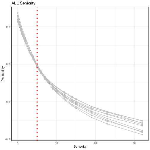
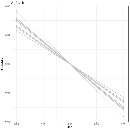
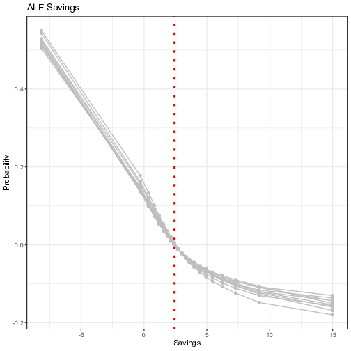
Figure 7: Visualization of the ensemble first-order Accumulated Local Plots. Each line represents the Accumulated Local Effects (ALE) of one trained neural network model. The y-axis represents the average prediction of the probability of default (1 = default) and the x-axis represents the values of the original independent variables. For the continuous variables, the vertical line in red represents the threshold computed by the FFT in Figure 5.
In order to account for more complex dynamics across features, Figure 8 shows the Partial Dependence of two variables at once for selected pairs. All possible pairs of exogenous variables have been tested. For the sake of parsimony, we show only the ones that are most relevant. As a general rule, one could implement a simple algorithm that would select only the pairs such that the difference between the maximum and the minimum probabilities over the parameters space is greater than a specified threshold. In our case, we selected the pairs with a gap of at least 20%. Each graph below has been computed by averaging the results of the 10 independent neural networks, showing the ensemble average impact.
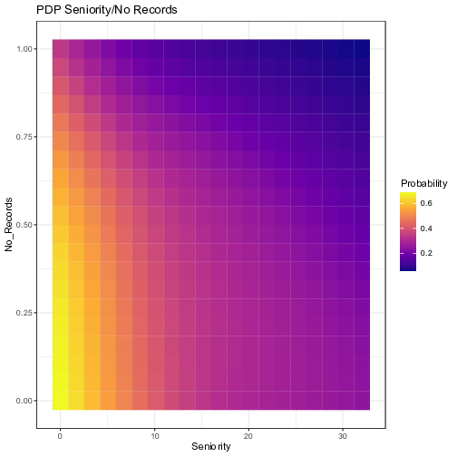
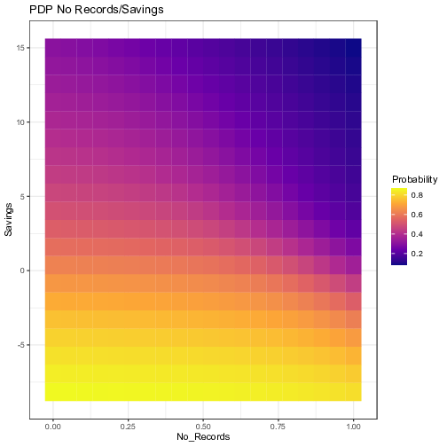
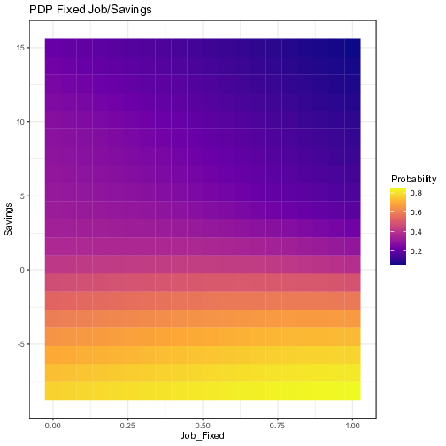
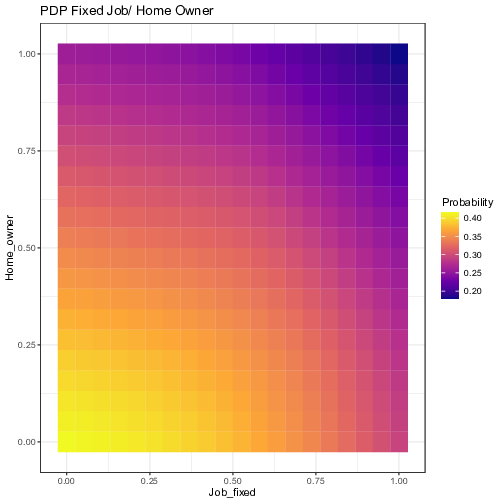
Figure 8: Visualization of the ensemble Partial Dependence Plots for selected pairs of variables. The axes represent the values of the original independent variables. The outputs of the partial dependence function, i.e. the prediction of the probability of default, from the 10 neural network models have been averaged for each grid value.
These interactions show what the FFT has potentially neglected by taking into account only one variable at a time, and making a decision at every node. For example, the first plot shows that an applicant with 5 years of experience (threshold given by the tree) coupled with no previous records of bad loans has twice as less chances of defaulting compared with someone with the same experience but with a previous record of default. The remaining plots also lead to similar conclusions for the other nodes of the tree. “Savings” seems to interact well with “No Records”; a minimum amount of savings is needed for the absence of previous default to have a significant decrease in the probability of a new default. Likewise, as stated before, relying solely on the presence of a fixed job is misleading, its interaction with “Savings” shows that having a fixed job has no positive effect unless savings levels are positive. On the opposite, being the owner of a house does not provide a significant additional boost to individuals with a fixed job.
These results are warning signals against making a decision too hastily with only one variable in sight. Therefore, these interaction plots demonstrate which variables inside the tree could be used in conjunction in order to discriminate further between the applicants and improve the accuracy of the predictions. This is the object of the next section.
The aim of this section is to build new interpretable models in order to optimize the tradeoff between interpretability and performance. Now, we want to keep the comprehensibility of our initial FFT model by minimizing the number of changes made, while increasing the performance of the initial tree.
From the analyses above, we can draw two lessons. Firstly, the sequence of variables found by the FFT may not be optimal. Both the first order PDP and the ALE plots (and in line with FFT results on the testing sample) point to the direction of a higher feature importance of “Savings” compared to “Home” and “Job”, the latter becoming then the least significant variable. A simple algorithm that ranks the variables given by the ALE plots and reorders the tree according to that ranking is then implemented. Thus, we reconstruct the initial FFT by simply shifting the order of our variables according to the hierarchy found by the ALE plots, while keeping the initial thresholds. Thus, our first augmented tree simply implies inverting the position of the variables “Home” and “Job”. Figure 9 shows the new augmented tree following this change.
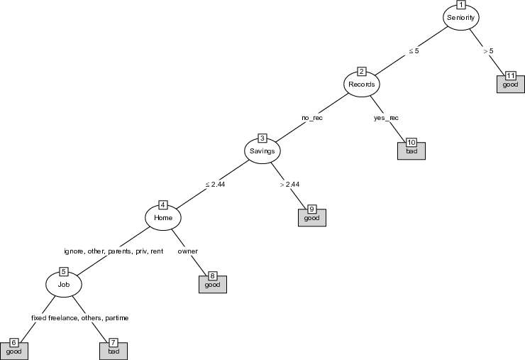
Figure 9: Visualization of the augmented FFT-1.
In a second step, we augment our model using the insights provided by the PDP second order effects (Figure 8). In search of a parsimonious augmented model, we decided to keep only the two most influential dyads of variables, namely the significant interactions between “Seniority” and “Records”, as well as the relation between “Job” and “Savings”.3 The first one concerns individuals with lower experience, i.e., applicants between 5 and 10 years; thus, we condition the approval of a loan to the absence of previous default. Moreover, we also add a final node at the bottom of the tree by requiring a positive level of savings before granting a loan to a fixed job applicant. Figure 10 shows the new augmented tree following those changes.
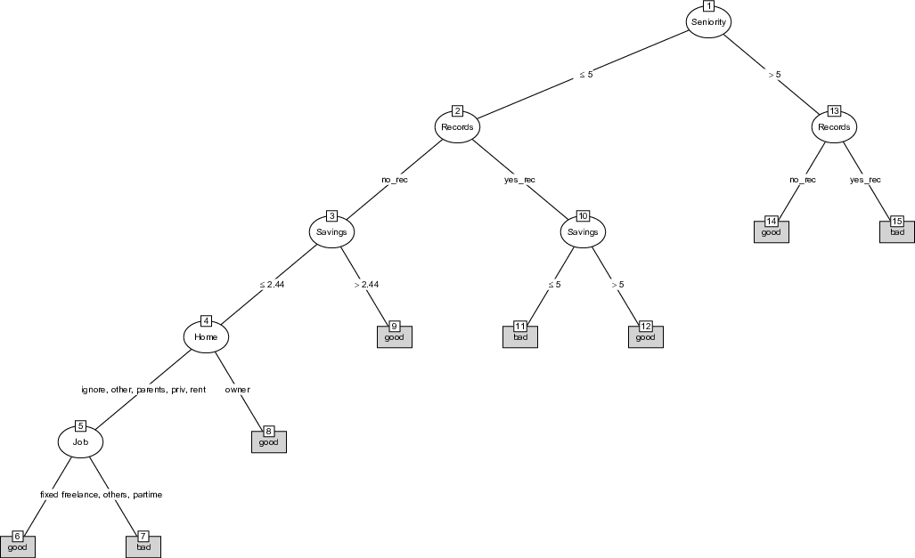
Figure 10: Visualization of the augmented FFT-2.
We are now in a position to compare the accuracy of our two augmented trees with several competing models. The original FFT and the standard decision tree (CART) will be our benchmarks for individual classifiers. Moreover, to assess the gap between the individual models and ensemble classifiers, we added traditional machine learning models like Logistic Regression, Random Forest, Support Vector Machine, and XGBoosting. We also predict default rates with the ensemble neural network (NN) models described in the Methodology. The ensemble output is the equally weighted average of the predictions of the 10 heterogeneous models. All the methodologies presented below have been tested 100 times with different training and testing samples. The outcome of all these classification models is then summarized in a confusion matrix. From the latter, we compare the accuracy of the predictions by computing several metrics on the testing samples. First, as a measure of absolute performance, we use the percentage of correct predictions. Moreover, we complement this measure with the sensitivity (percentage of cases with correct default rates) and specificity (percentage of cases with correct non-default rates) measures, having in mind that Type-1 error (granting a loan to an insolvent borrower), which is directly related to specificity, may be have a different impact than Type-2 error (refusing a loan to a solvent borrower), which is linked to sensitivity. The performances of the competing models are displayed in Table 1.
Table 1: Model accuracy (%) by type of model, sorted from the lowest to the highest absolute prediction. Bold highlights maximum of each column.
Model Absolute correct predictions % Sensitivity % Specificity % FFT 72.6 76.1 63.5 SVM All 73.4 98.9 7.5 SVM 5 73.5 90.5 30.1 CART All 75.1 91.9 28.9 CART (5) 75.4 88.5 45.4 Augmented FFT-1 76.6 92.4 36.4 Augmented FFT-2 76.6 90.2 41.9 XGBoost All 76.7 87.6 49.2 XGBoost 5 76.8 87.7 48.7 Ensemble ML (5) 77.1 89.6 45.7 RF (5) 77.3 94.4 33.0 Logistic Regression (5) 77.7 91.2 43.0 RF All 78.1 89.6 48.5 Ensemble ML (All) 78.8 89.4 52.5 Logistic Regression All 79.1 91.5 47.0
The best performing model, albeit by a small margin, is the logistic regression model followed closely with the Ensemble NN, all with the full set of variables. This result echoes previous findings on the outperformance of heterogeneous ensemble learning in Probability of Default (PD) modelling (Papouskova & Hajek, 2019). In absolute terms, the logistic regression model outperforms the simplest FFT by more than 6%, the CART models by 4%, and outperform the two augmented trees by only 2.5%. One could argue that the marginal gain is rather low though. This echoes the results in du Jardin (2018) who measured the average gain calculated over 31 studies to be 2.4% with only 10 being statistically significant. Table 2 shows the p-values following a test on the equality of proportions for each pair of competing models. The best models (logistic and ensemble NN), are significantly better than the FFT trees, the CART and SVM models; however, it is not significantly better than the other methodologies, the augmented trees included. Our augmented trees are significantly better than the FFT tree but do not significantly outperform the most complex CART models.
Table 2: P-values of a test for the difference in two proportions (absolute correct predictions in Table 1) Values are expressed in percentages.
Model
Having said that, a closer look at the results indicates that the benchmark FFT does a much better job at balancing sensitivity and specificity, which is not so surprising since the FFT has been designed to weigh the two components equally. Some models perform badly in terms of specificity, notably the two CART and SVM methodologies, as well as the smaller version of the Random Forest model, which may be problematic in practice. In that regard, the augmented trees also outperform the CART models by a significant margin, while being below the FFT level. The ensemble NN fares a bit better than the augmented trees, while being still significantly lower than the FFT tree.
Given that our dataset is unbalanced, i.e., with more non-defaulters than defaulters (71% vs. 29%), the outperformance of the different trees is then dependent upon the number of negative or positive exits until the last node, or the so-called “rake”.4 From our benchmark FFT, (3 positive exits vs. 3 negative exits), we showed that decreasing adequately the number of negative exits, as Augmented FFT-1 does (4 positive exits vs. 2 negative exits), has an immediate significant positive effect on the overall accuracy. However, as mentioned in Phillips et al. (2017), positive (negative) rake trees exhibit high sensitivity (specificity) at the expense of low specificity (sensitivity). Specificity is related to the Type-1 error (granting a loan to an insolvent borrower) that may be more important than Type-2 error (refusing a loan to a solvent borrower), which is in turn related to sensitivity. This pattern is visible in Augmented FFT-1, which with a positive rake suffers from low specificity. By adding another node in the latter and therefore partially rebalancing the relative number of exits, Augmented FFT-2 is less biased and shows higher specificity (5 positive exits vs. 3 negative exits) while maintaining a similar overall accuracy.
As explained in the Method section, one could modify the loss function in the NN ensemble (as well as other ML methods) to accommodate higher specificity, and then extract the new marginal contributions from the new ensemble models in search for new augmented trees. Interestingly, implementing the loss function as in Equation (4), i.e., changing the loss function to combine specificity and sensitivity in the ensemble ML model confirms the order of the variables given by our FFT benchmark model.5
Overall, the choice between the augmented trees and the competing models will be eventually dictated by the criterion that is the most relevant for the user. Nevertheless, we showed that, with much more simplicity than complex decision trees, a Fast and Frugal Tree augmented by explainable ML outputs is a step closer towards breaking the tradeoff between interpretability and performance.
The ability to understand how credit score models work emerges as a critical issue: individuals claim their right to explanation for significant decisions, and legislators around the world are granting this right as witnessed, for instance, by the Equal Credit Opportunity Act in the US and the General Data Protection Regulation in the EU. Based on the premise that the relationship between inputs and outputs of a machine-learning model, albeit accurate, can never be perfectly specified, interpretable machine learning ought to close the gap between misspecification and transparency. We have shown that if interpretable models are often good at measuring feature importance, post hoc explainability methods of opaque models, like PDP and ALE, are tools that equip decisions makers with a better understanding of the dynamics between variables. Moreover, combining these tools with an ensembling methodology provides an efficient and human friendly way to obtain Bayesian uncertainty estimations of the interpretable model’s thresholds and coefficients.
Our work contributes to the development of decision strategies in complex, ill-structured and dynamic conditions where the data characteristics involve complex interrelationships among variables, with first and second order interaction effects. Our findings reveal the complex influence of some variables on the probability of default of borrowers and the difficulty sometimes to assess their discriminant nature solely using interpretable classification tasks. In this article, we argue that highlighting first white-box models and then shedding light on black-box models, in a sequential approach that holds the characteristics of sparsity and explainability, is the future of machine learning interpretability.
Moreover, in the lending industry, decision makers have multiple, competing goals since they need to maximize the return on their capital while avoiding defaults, where many externalities can influence the probability of defaulting on the loan. Our methodology echoes the work of Zhao et al. (2021) on the causal interpretation of black box models, and thus opens the doors to the discovery of more structural models. However, considerable domain knowledge and deliberation may be needed to achieve causality in the sense of Pearl et al. (2018). Thus, we want to stress the importance of human intervention in augmenting machine-based intelligence. Having said that, for scalability reasons, human intervention should be called upon only when it is the most relevant; in our case, to interpret the new insights provided by Machine Learning explainable outputs. We believe that the ultimate objective of the interactions between humans and machines is to produce better comprehensible and justifiable models, which could be eventually used in an automated and actionable way by other human beings.
Indeed, in order to continuously improve the applicability and performance of our methodology, our business counterpart committed to apply the model develop in this project to a selection of real-life cases and share with us the results obtained.
Apley, D. W., & Zhu, J. (2019). Visualizing the effects of predictor variables in black box supervised learning models. ArXiv:1612.08468.
Apley, D. W., & Zhu, J. (2020). Visualizing the effects of predictor variables in black box supervised learning models. Journal of the Royal Statistical Society: Series B (Statistical Methodology), 82(4). https://doi.org/10.1111/rssb.12377.
Barredo Arrieta, A., Díaz-Rodríguez, N., del Ser, J., Bennetot, A., Tabik, S., Barbado, A., … Herrera, F. (2020). Explainable artificial intelligence (XAI): Concepts, taxonomies, opportunities and challenges toward responsible AI. Information Fusion, 58. https://doi.org/10.1016/j.inffus.2019.12.012.
Bertsimas, D., & Dunn, J. (2017). Optimal classification trees. Machine Learning, 106(7). https://doi.org/10.1007/s10994-017-5633-9.
Bertsimas, D., King, A., & Mazumder, R. (2016). Best subset selection via a modern optimization lens. The Annals of Statistics, 44(2). https://doi.org/10.1214/15-AOS1388.
Breiman, L. (2001). Random forests. Machine Learning, 45(1). https://doi.org/10.1023/A:1010933404324.
Breiman, L., Friedman, J. H., Olshen, R. A., & Stone, C. J. (2017). Classification and regression trees. Routledge. https://doi.org/10.1201/9781315139470.
Brighton, H., & Gigerenzer, G. (2015). The bias bias. Journal of Business Research, 68(8). https://doi.org/10.1016/j.jbusres.2015.01.061.
Burrell, J. (2016). How the machine ‘thinks’: Understanding opacity in machine learning algorithms. Big Data & Society, 3(1). https://doi.org/10.1177/2053951715622512.
Cabitza, F., Rasoini, R., & Gensini, G. F. (2017). Unintended consequences of machine learning in medicine. JAMA, 318(6). https://doi.org/10.1001/jama.2017.7797.
Chen, Y.-S., & Cheng, C.-H. (2013). Hybrid models based on rough set classifiers for setting credit rating decision rules in the global banking industry. Knowledge-Based Systems, 39. https://doi.org/10.1016/j.knosys.2012.11.004.
Coussement, K., & Benoit, D. F. (2021). Interpretable data science for decision making. Decision Support Systems, 150, 113664. https://doi.org/10.1016/j.dss.2021.113664.
Cowan, N. (2010). The Magical Mystery Four. Current Directions in Psychological Science, 19(1). https://doi.org/10.1177/0963721409359277.
Crook, J. N., Edelman, D. B., & Thomas, L. C. (2007). Recent developments in consumer credit risk assessment. European Journal of Operational Research, 183(3). https://doi.org/10.1016/j.ejor.2006.09.100.
Deku, S. Y., Kara, A., & Molyneux, P. (2016). Access to consumer credit in the UK. The European Journal of Finance, 22(10). https://doi.org/10.1080/1351847X.2015.1019641.
Derelioğlu, G., & Gürgen, F. (2011). Knowledge discovery using neural approach for SME’s credit risk analysis problem in Turkey. Expert Systems with Applications, 38(8). https://doi.org/10.1016/j.eswa.2011.01.012.
Dietvorst, B. J., Simmons, J. P., & Massey, C. (2015). Algorithm aversion: People erroneously avoid algorithms after seeing them err. Journal of Experimental Psychology: General, 144(1). https://doi.org/10.1037/xge0000033.
du Jardin, P. (2018). Failure pattern-based ensembles applied to bankruptcy forecasting. Decision Support Systems, 107, 64–77. https://doi.org/10.1016/j.dss.2018.01.003.
Dwork, C., Hardt, M., Pitassi, T., Reingold, O., & Zemel, R. (2012). Fairness through awareness. Proceedings of the 3rd Innovations in Theoretical Computer Science Conference on - ITCS ’12. New York, New York, USA: ACM Press. https://doi.org/10.1145/2090236.2090255.
Finlay, S. (2011). Multiple classifier architectures and their application to credit risk assessment. European Journal of Operational Research, 210(2). https://doi.org/10.1016/j.ejor.2010.09.029.
Florez-Lopez, R., & Ramon-Jeronimo, J. M. (2015). Enhancing accuracy and interpretability of ensemble strategies in credit risk assessment. A correlated-adjusted decision forest proposal. Expert Systems with Applications, 42(13). https://doi.org/10.1016/j.eswa.2015.02.042.
Friedman, J. H. (2001). Greedy function approximation: A gradient boosting machine. The Annals of Statistics, 29(5), 1189–1232.
Friedman, J., Hastie, T., & Tibshirani, R. (2010). Regularization paths for generalized linear models via coordinate descent. Journal of Statistical Software, 33(1). https://doi.org/10.18637/jss.v033.i01.
Fu, R., Huang, Y., & Singh, P. V. (2021). Crowds, lending, machine, and bias. Information Systems Research. https://doi.org/10.1287/isre.2020.0990.
Gadzinski, G., & Castello, A. (2020). Fast and frugal heuristics augmented: When machine learning quantifies Bayesian uncertainty. Journal of Behavioral and Experimental Finance, 26. https://doi.org/10.1016/j.jbef.2020.100293.
Gal, Y., & Ghahramani, Z. (2016). Dropout as a Bayesian approximation: representing model uncertainty in deep learning. Proceedings of the 33rd International Conference on Machine Learning - Volume 48, 1050–1059. New York, NY, USA.
Gilpin, L. H., Bau, D., Yuan, B. Z., Bajwa, A., Specter, M., & Kagal, L. (2018). Explaining explanations: An overview of interpretability of machine learning. 2018 IEEE 5th International Conference on Data Science and Advanced Analytics (DSAA). IEEE. https://doi.org/10.1109/DSAA.2018.00018.
Greenwell, B. M. (2017). pdp: An R package for constructing partial dependence plots. The R Journal, 9(1). https://doi.org/10.32614/RJ-2017-016.
Hand, D. J. (2006). Classifier technology and the illusion of progress. Statistical Science, 21(1). https://doi.org/10.1214/088342306000000060.
Hardt, M., & Talwar, K. (2010). On the geometry of differential privacy. Proceedings of the 42nd ACM Symposium on Theory of Computing - STOC ’10. New York, New York, USA: ACM Press. https://doi.org/10.1145/1806689.1806786.
Harris, T. (2015). Credit scoring using the clustered support vector machine. Expert Systems with Applications, 42(2). https://doi.org/10.1016/j.eswa.2014.08.029.
Hayashi, Y., & Takano, N. (2020). One-dimensional convolutional neural networks with feature selection for highly concise rule extraction from credit scoring datasets with heterogeneous attributes. Electronics, 9(8). https://doi.org/10.3390/electronics9081318.
Jang, H. (2019). A decision support framework for robust R&D budget allocation using machine learning and optimization. Decision Support Systems, 121. https://doi.org/10.1016/j.dss.2019.03.010.
Jussupow, E., Spohrer, K., Heinzl, A., & Gawlitza, J. (2021). Augmenting medical diagnosis decisions? An investigation into physicians’ decision-making process with artificial intelligence. Information Systems Research. https://doi.org/10.1287/isre.2020.0980.
Karatzoglou, A., Meyer, D., & Hornik, K. (2006). Support vector machines in R. Journal of Statistical Software, 15(9). https://doi.org/10.18637/jss.v015.i09.
Kraus, M., & Feuerriegel, S. (2019). Forecasting remaining useful life: Interpretable deep learning approach via variational Bayesian inferences. Decision Support Systems, 125. https://doi.org/10.1016/j.dss.2019.113100.
Krishnan, M. (2020). Against interpretability: A critical examination of the interpretability problem in machine learning. Philosophy & Technology, 33(3). https://doi.org/10.1007/s13347-019-00372-9.
Lakshminarayanan, B., Pritzel, A., & Blundell, C. (2017). Simple and scalable predictive uncertainty estimation using deep ensembles. Proceedings of the 31st International Conference on Neural Information Processing Systems, 6405–6416. Long Beach, California, USA.
Lessmann, S., Baesens, B., Seow, H.-V., & Thomas, L. C. (2015). Benchmarking state-of-the-art classification algorithms for credit scoring: An update of research. European Journal of Operational Research, 247(1). https://doi.org/10.1016/j.ejor.2015.05.030.
Licklider, J. C. R. (1960). Man-computer symbiosis. IRE Transactions on Human Factors in Electronics, HFE-1(1), 4–11. https://doi.org/10.1109/THFE2.1960.4503259.
Lundberg, S. M., & Lee, S.-I. (2017). A unified approach to interpreting model predictions. Advances in Neural Information Processing Systems, 4765–4774.
Luo, Y., Tseng, H.-H., Cui, S., Wei, L., ten Haken, R. K., & el Naqa, I. (2019). Balancing accuracy and interpretability of machine learning approaches for radiation treatment outcomes modeling. BJR|Open, 1(1). https://doi.org/10.1259/bjro.20190021.
Martignon, L., Katsikopoulos, K. v., & Woike, J. K. (2008). Categorization with limited resources: A family of simple heuristics. Journal of Mathematical Psychology, 52(6). https://doi.org/10.1016/j.jmp.2008.04.003.
Martignon, L., Vitouch, O., Takezawa, M., & Forster, M. R. (2005). Naive and yet enlightened: From natural frequencies to fast and frugal decision trees. In Thinking: Psychological Perspectives on Reasoning, Judgment and Decision Making. Chichester, UK: John Wiley & Sons, Ltd. https://doi.org/10.1002/047001332X.ch10.
Miller, G. A. (1956). The magical number seven, plus or minus two: Some limits on our capacity for processing information. Psychological Review, 63(2). https://doi.org/10.1037/h0043158.
Moreira, C., Chou, Y.-L., Velmurugan, M., Ouyang, C., Sindhgatta, R., & Bruza, P. (2021). LINDA-BN: An interpretable probabilistic approach for demystifying black-box predictive models. Decision Support Systems, 150, 113561. https://doi.org/10.1016/j.dss.2021.113561.
Murdoch, W. J., Singh, C., Kumbier, K., Abbasi-Asl, R., & Yu, B. (2019). Definitions, methods, and applications in interpretable machine learning. Proceedings of the National Academy of Sciences, 116(44). https://doi.org/10.1073/pnas.1900654116.
Olson, D. L., Delen, D., & Meng, Y. (2012). Comparative analysis of data mining methods for bankruptcy prediction. Decision Support Systems, 52(2). https://doi.org/10.1016/j.dss.2011.10.007.
Papouskova, M., & Hajek, P. (2019). Two-stage consumer credit risk modelling using heterogeneous ensemble learning. Decision Support Systems, 118, 33–45. https://doi.org/10.1016/j.dss.2019.01.002.
Parpart, P., Jones, M., & Love, B. C. (2018). Heuristics as Bayesian inference under extreme priors. Cognitive Psychology, 102. https://doi.org/10.1016/j.cogpsych.2017.11.006.
Pearce, T., Leibfried, F., & Brintrup, A. (2020). Uncertainty in neural networks: Approximately Bayesian ensembling. Proceedings of the Twenty Third International Conference on Artificial Intelligence and Statistics - Volume 108, 234–244.
Pearl, J., & Mackenzie, D. (2018). The book of why: The new science of cause and effect (First Edition). Basic Books.
Phillips, N. D., Neth, H., Woike, J. K., & Gaissmaier, W. (2017). FFTrees: A toolbox to create, visualize, and evaluate fast-and-frugal decision trees. Judgment and Decision Making, 12(4), 344–368.
Pintelas, E., Livieris, I. E., & Pintelas, P. (2020). A grey-box ensemble model exploiting black-box accuracy and white-box intrinsic interpretability. Algorithms, 13(1). https://doi.org/10.3390/a13010017.
Ribeiro, M. T., Singh, S., & Guestrin, C. (2016). “Why should I trust you?” Proceedings of the 22nd ACM SIGKDD International Conference on Knowledge Discovery and Data Mining. New York, NY, USA: ACM. https://doi.org/10.1145/2939672.2939778.
Rudin, C. (2019). Stop explaining black box machine learning models for high stakes decisions and use interpretable models instead. Nature Machine Intelligence, 1(5). https://doi.org/10.1038/s42256-019-0048-x.
Shin, D. (2020). User perceptions of algorithmic decisions in the personalized AI system: Perceptual evaluation of fairness, accountability, transparency, and explainability. Journal of Broadcasting & Electronic Media, 64(4), 541–565. https://doi.org/10.1080/08838151.2020.1843357.
Shin, D. (2021a). Embodying algorithms, enactive artificial intelligence and the extended cognition: You can see as much as you know about algorithm. Journal of Information Science, 016555152098549. https://doi.org/10.1177/0165551520985495.
Shin, D. (2021b). The effects of explainability and causability on perception, trust, and acceptance: Implications for explainable AI. International Journal of Human-Computer Studies, 146, 102551. https://doi.org/10.1016/j.ijhcs.2020.102551.
Shin, D. (2021c). The perception of humanness in conversational journalism: An algorithmic information-processing perspective. New Media & Society, 146144482199380. https://doi.org/10.1177/1461444821993801.
Shin, D. (2021d). Why does explainability matter in news analytic systems? Proposing explainable analytic journalism. Journalism Studies, 22(8), 1047–1065. https://doi.org/10.1080/1461670X.2021.1916984.
Shin, D. (2022). How do people judge the credibility of algorithmic sources? AI & SOCIETY, 37(1), 81–96. https://doi.org/10.1007/s00146-021-01158-4.
Subramania, H. S., & Khare, V. R. (2011). Pattern classification driven enhancements for human-in-the-loop decision support systems. Decision Support Systems, 50(2). https://doi.org/10.1016/j.dss.2010.11.003.
Sun, J., Li, H., Huang, Q.-H., & He, K.-Y. (2014). Predicting financial distress and corporate failure: A review from the state-of-the-art definitions, modeling, sampling, and featuring approaches. Knowledge-Based Systems, 57. https://doi.org/10.1016/j.knosys.2013.12.006.
Tomczak, J. M., & Zięba, M. (2015). Classification restricted Boltzmann machine for comprehensible credit scoring model. Expert Systems with Applications, 42(4). https://doi.org/10.1016/j.eswa.2014.10.016.
Topuz, K., & Delen, D. (2021). A probabilistic Bayesian inference model to investigate injury severity in automobile crashes. Decision Support Systems, 150, 113557. https://doi.org/10.1016/j.dss.2021.113557.
Varshney, K. R., & Alemzadeh, H. (2017). On the safety of machine learning: Cyber-physical systems, decision sciences, and data products. Big Data, 5(3). https://doi.org/10.1089/big.2016.0051.
Waa, J. van der, Schoonderwoerd, T., Diggelen, J. van, & Neerincx, M. (2020). Interpretable confidence measures for decision support systems. International Journal of Human-Computer Studies, 144. https://doi.org/10.1016/j.ijhcs.2020.102493.
Zhao, Q., & Hastie, T. (2021). Causal interpretations of black-box models. Journal of Business & Economic Statistics, 39(1), 272–281. https://doi.org/10.1080/07350015.2019.1624293.
Appendix: List of Independent Variables
Default Default dummy variable Seniority Job seniority (years) Home Type of home ownership (3 dummies) Time Time of requested loan Age Client’s age Marital Marital status (3 dummies) Records Existence of negative records Job Type of job (3 dummies) Expenses Amount of expenses Income Amount of income Assets Amount of assets Debt Amount of debt Amount Amount requested of loan Finrat Financial rating
Copyright: © 2022. The authors license this article under the terms of the Creative Commons Attribution 3.0 License.
This document was translated from LATEX by HEVEA.