Judgment and Decision Making, Vol. 17, No. 3, May 2022, pp. 487-512
Explaining human sampling rates across different decision domains
Didrika S. van de Wouw* #
Ryan T. McKay#
Bruno B. Averbeck$
Nicholas Furl$
|
Abstract:
Undersampling biases are common in the optimal stopping literature, especially for economic full choice problems. Among these kinds of number-based studies, the moments of the distribution of values that generates the options (i.e., the generating distribution) seem to influence participants’ sampling rate. However, a recent study reported an oversampling bias on a different kind of optimal stopping task: where participants chose potential romantic partners from images of faces (Furl et al., 2019). The authors hypothesised that this oversampling bias might be specific to mate choice. We preregistered this hypothesis and so, here, we test whether sampling rates across different image-based decision-making domains a) reflect different over- or undersampling biases, or b) depend on the moments of the generating distributions (as shown for economic number-based tasks). In two studies (N = 208 and N = 96), we found evidence against the preregistered hypothesis. Participants oversampled to the same degree across domains (compared to a Bayesian ideal observer model), while their sampling rates depended on the generating distribution mean and skewness in a similar way as number-based paradigms. Moreover, optimality model sampling to some extent depended on the the skewness of the generating distribution in a similar way to participants. We conclude that oversampling is not instigated by the mate choice domain and that sampling rate in image-based paradigms, like number-based paradigms, depends on the generating distribution.
Keywords: optimal stopping, decision making, Bayesian modelling, bias
1 Introduction
An optimal stopping problem can be defined as a situation in which a decision maker has to choose when to stop searching for more information and take a given action. For example, imagine an agent who has one week to find the best flat (apartment) at the best price, can visit one flat per day, and must accept or reject the flat at the visit. This is because, after leaving a visit, the flat is likely to be sold to someone else, so cannot be "recalled" by the agent once rejected. Optimal stopping problems have long held the fascination of scholars, particularly mathematicians, who were determined to prove that optimal solutions to these kinds of problems exist (for historical reviews, see Freeman, 1983,Ferguson, 1989).
Within this paper we focus on a specific and simple version of the so-called full information problem, where the actual values of the options are presented, the distributions that generate the option values (i.e., the generating distributions) are familiar to participants, there is no extrinsic cost-to-sample, there is no recall of rejected options, and decision outcomes provide a reward equal to their value (Gilbert and Mosteller, 1966,Lee, 2006,Guan et al., 2014,Shu, 2008,Abdelaziz and Krichen, 2006,Hill, 2009). For example, imagine our flat-hunting agent (like most informed shoppers) already possesses useful prior knowledge about the (normal) distribution of flat values on the market, incurs no extra travel or time costs to visit a new flat, learns the exact value of each flat (and not merely its relative rank) upon visiting it, and better valued-flats lead to a more rewarding outcomes (instead of merely the best-ranked flat being rewarding). These full information decision problems are solved computationally using a backwards induction algorithm, which predicts the values of future options based on a known distribution that generates the option values (Gilbert and Mosteller, 1966,Costa and Averbeck, 2015,Furl et al., 2019,Cardinale et al., 2021). These models of optimality are programmed by researchers with the mean and variance of the assumed-to-be-normal generating distribution (or the prior of this distribution), which the researchers assume the participants are using (Gilbert and Mosteller, 1966,Costa and Averbeck, 2015). Other types of optimal stopping problems exist that require somewhat different computational solutions, but those are outside the scope of this paper (e.g., Goldstein et al., 2020,Zwick et al., 2003,Van der Leer et al., 2015).
Previous research has found evidence that participants commonly undersample compared to optimality in our focus case of simple full information problems (Costa and Averbeck, 2015,Cardinale et al., 2021). Even further, this undersampling bias also been found in multiple closely-related optimal stopping problems that go beyond our focus, including the classic secretary task (Seale and Rapoport, 1997,Bearden et al., 2006), numerical optimal stopping tasks (Guan et al., 2014,Guan and Lee, 2018,Kahan et al., 1967,Shapira and Venezia, 1981), and even the beads task (Furl and Averbeck, 2011,Van der Leer et al., 2015,Hauser et al., 2017,Hauser et al., 2018). In addition to undersampling biases, human sampling rates can be affected by other factors such as sequence length (Goldstein et al., 2020,Costa and Averbeck, 2015,Cardinale et al., 2021), cost-to-sample (Zwick et al., 2003,Costa and Averbeck, 2015), or the moments of the distribution that generates the option values (i.e., many high/low value options; Guan et al., 2014,Guan and Lee, 2018,Baumann et al., 2020,Guan et al., 2020). The latter factor - moments of the generating distribution - is a focus of the current paper.
However, a recent study reported an oversampling bias in a different decision-making domain within the same full information modelling framework. In a mate choice decision scenario, participants searched for the most attractive date from a series of faces (Furl et al., 2019). (Furl et al., 2019) hypothesised that the oversampling bias on this non-economic, image-based task might be specific to the mate choice decision-making domain. Their hypothesis was based on behavioural ecology research which suggests that animals use high thresholds for mate choice (Ivy and Sakaluk, 2007,Backwell and Passmore, 1996,Milinski and Bakker, 1992). Furthermore, (Furl et al., 2019) reported that a computational model that incorporated such a high-threshold bias best described participants’ sampling behaviour.
Here, we continue to examine influences on human sampling rate in image-based optimal stopping tasks with two main hypotheses. (Furl et al., 2019) have found an oversampling bias in mate choice decisions, so firstly, we want to investigate if other naturalistic domains also lead to the same bias. The second hypothesis is based on previous studies of the number-based full information task which show that a more positively skewed generating distribution can increase sampling rate (Baumann et al., 2020). To date, this hypothesis has been tested in number-based domains only, and has yet to be tested in image-based domains. For the two purposes outlined above, we have chosen three image-based decision-making domains: faces (replication), food, and holiday destinations.
2 Materials and methods
We conducted two studies aimed at convergent results; one online (Study 1) and one in a classroom setting (Study 2). The data analysis plan for our online study was preregistered before data collection, and is openly available on the AsPredicted pre-registration website.1 Our classroom study was not separately pre-registered but followed the same data analysis protocol as pre-registered for Study 1. Methods for Study 1 and Study 2 were nearly identical, as outlined below.
2.1 Study 1
2.1.1 Participants
For our first study, 225 participants were recruited through the online recruitment service Prolific (Prolific, 2014). Two participant prerequisites were set, the first being age (between 18 and 35), as this roughly matched the age range of the faces shown in the study. The second prerequisite was nationality (either United Kingdom (UK), Ireland, United States (US), Canada, Australia, or New Zealand), which was set under the assumption that participants with these nationalities would have a good command of the English language, and would therefore be able to understand the instructions and the informed consent form. Each participant was randomly assigned to one of three conditions (N = 75 each), with each condition corresponding to a different decision domain. Participants received a flat fee as compensation for completing the study, with the entire study lasting about 15 minutes.
2.1.2 Paradigm
Gorilla Experiment Builder (Anwyl-Irvine et al., 2020) was used to create and host our studies. The paradigm for all three domains (faces, food and holiday destinations) was very similar, and inspired by the methods used across the three studies described in (Furl et al., 2019). The paradigm consisted of two phases; a rating phase and a sequence phase (i.e., the optimal stopping task). Before commencing the study, participants in the faces domain were asked to choose whether they would like to rate (and date) males or females. Based on their answers, each was shown either male or female faces throughout the study.
For the faces domain, 90 faces were randomly selected from a larger set of 426 images, the same set used in Study 2 of (Furl et al., 2019). The set of 90 food images was randomly selected from a larger set of 1314 images (Blechert et al., 2019). The image numbers corresponding to the food images that were used in this study can be found in the Supplementary Materials (Section S1). The set of holiday destination images was randomly selected from a royalty-free image database (www.shutterstock.com). Search terms that were used included, for example, ‘holiday destination’, ‘holiday’, ‘travel destination’, ‘travelling’, and ‘European city’. Stimulus dimensions of the three stimulus sets were kept as homogeneous as possible. For example, all images were cropped to the same size (1200 pixels) and the same shape (square). Other stimulus dimensions such as hue and saturation were not further controlled for, as differences can be expected both within and between domains.
In phase one of the study, participants rated 180 images in total (90 unique images, all rated twice) using a slider scale ranging from very unattractive (value 1) to very attractive (value 100). Consistent with previous studies of full information problems (Costa and Averbeck, 2015,Cardinale et al., 2021), the prior of the option-generating distribution was configured with the mean and variance of the generating distribution. In our case, as in (Furl et al., 2019), this means the distribution of subjective values (attractiveness ratings). Using personalised ratings ensures that the likelihood of an image being chosen is not influenced by individual differences in attractiveness preferences (Furl et al., 2019), as the same prior distribution of values was available for learning to both agents, that is, the participants and the optimality model against which we compare the participants (see Section 2.4). Sliders were made invisible until first click to reduce slider biases (Matejka et al., 2016), and the slider’s current selected value was shown for increased precision. A progress bar was shown at the bottom of the screen to visualise participants’ progression. An attention check was included in phase one to compensate for the unsupervised nature of online data collection (see Supplementary Materials, Section S2). Final attractiveness ratings were computed from the mean of the two ratings, which previous work has found to be sufficient for detecting oversampling on the facial attractiveness paradigm (Furl et al., 2019, Study 3) and which shortened the duration of our study to suit online presentation. Internal consistency between the two ratings, measured using Cronbach’s alpha, was acceptable (Taber, 2018), confirming that participants were consistent in their ratings of images (female faces: α = 0.848, male faces: α = 0.882, food: α = 0.954, holiday destinations: α = 0.926).
In the second phase, participants were shown six sequences of eight images each, shown one at a time. Images were randomly sampled from the entire distribution of images that had been rated in phase one. Participants were instructed to attempt to choose the most attractive option from the sequence that they could, with the restriction that they could not return to a previously rejected option. The number of options remaining was shown at the top of the screen, and the rejected options were shown at the bottom of the screen. When a participant made a choice, they had to advance through a series of grey squares that replaced the remaining images. This ensured that participants could not finish the experiment early by choosing an early option. Adding grey squares does not alter participants’ sampling behaviour: (Furl et al., 2019) found the same results on the facial attractiveness paradigm with the implementation of grey squares (Studies 2 and 3) and without (Study 1). The entire study was self-paced - participants advanced by using their mouse to click on the buttons on the screen. If the last option in the sequence was reached, that option became their choice by default. After finishing a sequence, participants were directed to a feedback screen displaying the participant’s chosen image, and the text: “Here is your [new date / next meal / next holiday destination]! How rewarding is your choice?”. Participants responded to this question using a slider scale ranging from not rewarding (value 1) to very rewarding (value 100). The feedback screen was included to provide feedback about the quality of the participants’ choice by asking them to reflect upon its reward value before moving onto the next sequence, and responses were not further analysed. Next, participants were directed to a screen asking them: “Ready for the next sequence?”. Participants responded by clicking a button saying: “I’m ready!”.
The two key dependent variables of interest are the position of the chosen image in the sequence (i.e., number of samples), and the rank of the chosen image (out of the images in the sequence). Both variables are a mean value over six sequences for each participant.
2.2 Study 2
A second study was conducted in a laboratory setting to replicate the results of Study 1 (which was conducted online) and thus bolster our findings. Opportunity sampling was used to recruit 96 participants during an Open Day at Royal Holloway, University of London. This sample size was sufficiently large, as a power analysis based on the outcomes of Study 1 indicated that for Study 2, a total sample size of 70 participants was sufficient for 95% power. Participants were randomly allocated to one of three domains, with final numbers being 32 in faces, 28 in food, and 36 in holiday destinations. Participants did not receive any monetary compensation for their participation.
2.3 Paradigm
Study 2 used a shortened, but otherwise identical version of the paradigm described in Section 2.1.2. The reason it was shortened was because of time constraints related to the recruitment format (during a University Open Day). As such, the two key differences between Study 2 and Study 1 are 1) participants in Study 2 rated every image only once, and 2) the attention check was removed in Study 2 as the study was conducted in a more controlled setting. The shortened version of the paradigm may introduce more noise in the data, which could reduce our ability to detect a result. Despite this, we found no differences in the results due to the shortened format.
2.4 Optimality model
Participants’ sampling behaviour was compared to a Bayesian ideal observer model (Costa and Averbeck, 2015), where performance is Bayesian optimal and the cost-to-sample parameter2 was fixed to zero. This model has previously been used by e.g., (Costa and Averbeck, 2015), (Furl et al., 2019) and (Cardinale et al., 2021), and is the same as the model of (Gilbert and Mosteller, 1966) in that both assume that options are sampled from a normal option generating distribution with known mean and variance, and both use a backwards induction algorithm to compute the value of sampling again, which is compared to the value of the current option. The Bayesian optimality model enhances the original Gilbert and Mosteller model by adding to it 1) a generating distribution that is initialised with a prior distribution which is then updated after each new sample using Bayes’ rule, 2) a cost-to-sample parameter (here set to zero), and 3) functionality for the researcher to apply any arbitrary reward function to the choice outcomes. Mathematically, the model is based on a discrete time Markov decision process with continuous states. Theoretically, at each position in the sequence, the optimality model computes the respective values for choosing the option and declining the option, and chooses the one with the highest value. To calculate the value of either taking or declining an option in a sequence the model computes the action value Q as:
|
| | Qt | ⎛
⎝ | st,a = take | ⎞
⎠ | = rt | ⎛
⎝ | st,a | ⎞
⎠ | Qt | ⎛
⎝ | st,a = decline | ⎞
⎠ | = | ∫ | | pt | ⎛
⎝ | j ∣ st,a | ⎞
⎠ | ut+1(j) dj.
|
|
(1) |
The key computations for the optimality model, as seen in equation 1, are utility (equation 2) and reward values (equation 3). The model uses backwards induction to derive utilities that could result from further sampling (equation 4).
|
ut | ⎛
⎝ | st | ⎞
⎠ | = | | | ⎧
⎪
⎨
⎪
⎩ | rt | ⎛
⎝ | st,a | ⎞
⎠ | + | ∫ | | pt | ⎛
⎝ | j ∣ st,a | ⎞
⎠ | ut+1(j) dj
| ⎫
⎪
⎬
⎪
⎭ | (2) |
The utility u of the state s at sample t is the value of the best action a, which depends on reward value r, the cost-to-sample Cs, and the probabilities of outcomes j of subsequent states, weighted by their utilities. i represents each option in a sequence.
|
| | rt | ⎛
⎝ | st, a = accept | ⎞
⎠ | = | | p | ⎛
⎝ | rank = i | ⎞
⎠ | * R | ⎛
⎝ | i + (h−1) | ⎞
⎠ | rt | ⎛
⎝ | st, a = decline | ⎞
⎠ | = Cs
|
|
(3) |
Our optimality model adds to the Gilbert and Mosteller model a function R, which maps the rank of each option to the amount of reward gained when choosing an option of that rank. We assumed that participants followed our instructions and tried to choose the option with the highest subjective value possible. The corresponding model, if it followed these instructions, would therefore gain a reward commensurate with the subjective value (rating) of the chosen option. That is, we assigned to R(1) the rating of the highest ranked option, R(2) the rating of the second highest ranked item, and so on. This reward function resembles the classic Gilbert and Mosteller model, which also attempts to maximise the option value of its choices. h represents the relative rank of the current option. When considering final sequence position N, the model computes final utilities as:
|
uN | ⎛
⎝ | sN | ⎞
⎠ | = r | ⎛
⎝ | sN | ⎞
⎠ | for all sN∈ N,
(4) |
and working backwards from N, we use equation 2 to compute utilities at every sequence position t.
The value for declining an option can be considered the choice threshold, as no option is chosen unless the value for choosing an option exceeds the value for declining an option. The choice threshold is dynamic, and can change depending on the position in the sequence. The model received as input for each participant the values of the sequence options as presented to the participant in phase two, with each sequence value comprising the participant’s individual rating of the option. To approximate normality, ratings were log transformed. Input and parameter settings for the optimality model described here apply to all analyses in this paper.
2.5 Data analysis
The comparison of participants’ sampling behaviour to the optimality model was done using MATLAB version 2015b (MATLAB, 2015). Statistical tests were performed using RStudio (RStudioTeam, 2020). For all analyses, a p value of < .05 was considered significant. Additionally, to allow evidence for the null hypothesis to be quantified, we show the Bayes factors for mean number of samples and mean rank as well. Bayesian t-tests were calculated using the BayesFactor package (Morey and Rouder, 2018), within the R environment. We follow guidelines provided by (Lee and Wagenmakers, 2013) and (Wagenmakers et al., 2018) to interpret Bayes factors, with BF10 > 100 being interpreted as extreme or decisive evidence for the alternative hypothesis, and BF10 < .01 indicating evidence in favour of the null model (no differences between means).
3 Results
3.1 Study 1
After the removal of any outliers (see Supplementary Materials, Section S2.1), the final number of participants in each domain was 68 for faces, 72 for food, and 68 for holiday destinations (for demographic statistics, see Table S1 in the Supplementary Materials). In the facial attractiveness domain, the majority of participants chose to rate faces of the opposite sex (89.7%).
Because we were interested in testing the hypothesis proposed by (Furl et al., 2019) that oversampling bias is specific to the mate choice domain, we pre-registered the hypothesis that there would be a significant domain by agent interaction. We therefore implemented a 3x2 factorial ANOVA to compare the differential effects of our two agents (participants and model) across the three domains. We found that the domain by agent interactions for the mean number of samples and the mean rank of the chosen option did not reach significance (Table 1), so there was no evidence of a difference in sampling bias between domains. This is confirmed by the Bayes factor analysis, which showed that there was no evidence that the full model (domain + agent + domain by agent) was better than just the domain + agent model (BF10 = 0.260). In fact, there was extreme evidence for the domain + agent model (BF > 100). This Bayesian analysis, therefore, provides positive evidence for the absence of our pre-registered domain by agent interaction.
| Table 1: 3x2 factorial ANOVA describing the main effects and interaction effects for the mean number of samples and the mean rank of the chosen option, in both Study 1 and Study 2. Degrees of freedom is abbreviated as df. |
| | Study 1 | Study 2 |
| | df | F | p | df | F | p |
| Number of samples | | | | | | |
| Agent | (1, 406) | 240.75 | <.001 | (1, 185) | 159.27 | <.001 |
| Domain | (2, 406) | 46.83 | <.001 | (2, 185) | 27.81 | <.001 |
| Agent*Domain | (2, 406) | 1.77 | 0.171 | (2, 185) | 3.70 | 0.023 |
| Rank | | | | | | |
| Agent | (1, 408) | 232.53 | <.001 | (1, 186) | 18.57 | <.001 |
| Domain | (2, 408) | 7.43 | <.001 | (2, 186) | 1.76 | 0.175 |
| Agent*Domain | (2, 408) | 0.97 | 0.382 | (2, 186) | 6.94 | 0.001 |
Because the domain by agent interaction effect was not observed, this meant that, on average, the sampling rates of the two agents (participants and model) varied in the same way across domains. Indeed, when looking at sampling biases, we found evidence that despite variations in sampling rate for both agents across the domains (Figure 1), participants oversampled in each of our three domains when tested separately (Table 2), and achieved lower ranks than the optimality model (Figure 2, Table 2). Bayes factor t-tests supported this finding, showing extreme evidence for a difference between participants and the optimality model for the mean number of samples as well as the mean rank for each of the three domains (Table 3). Collapsing over agents, agents on average sampled more and achieved higher ranks in the faces domain than in either of the other two domains. Furthermore, agents on average sampled more in the food domain than in the holiday destinations domain (Table 4).
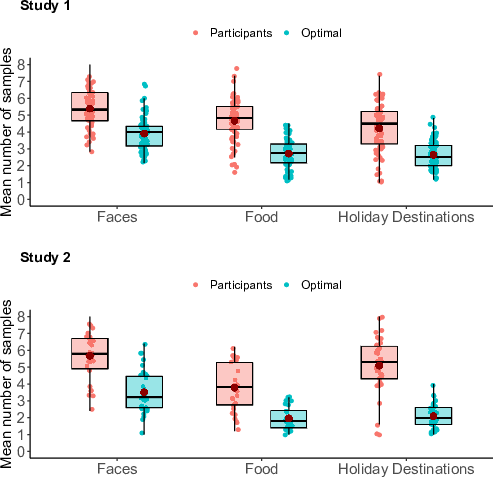
| Figure 1: Box plots and raw jittered data points for the mean number of samples for participants versus the optimality model, grouped by domain. The red dots represent the mean, horizontal black lines represent the median, boxes show the 25% and 75% quantiles, and the whiskers represent the 95% confidence intervals. |
| Table 2: Post hoc Friedman’s tests (Bonferroni corrected for the three domains) to test for differences between agents in each individual domain, in both Study 1 and Study 2. |
| | Study 1 | Study 2 |
|
| Number of samples | | |
| Faces | < .001 | < .001 |
| Food | < .001 | < .001 |
| Holidays | < .001 | < .001 |
|
| Rank | | |
| Faces | < .001 | < .001 |
| Food | < .001 | .450 |
| Holidays | < .001 | .304 |
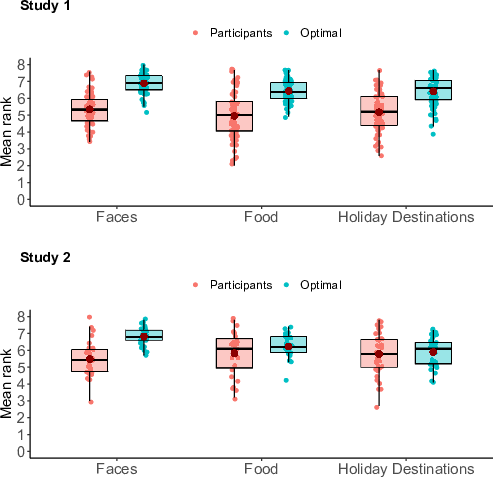
| Figure 2: Box plots and raw jittered data points for the mean rank of the chosen option for participants versus the optimality model, grouped by domain. The red dots represent the mean, horizontal black lines represent the median, boxes show the 25% and 75% quantiles, and the whiskers represent the 95% confidence intervals. |
| Table 3: Bayes factor (BF10) describing the difference between agents for the mean number of samples and the mean rank of the chosen option, for each of the three domains. |
| | Study 1 | Study 2 |
|
| Number of samples | | |
| Faces | BF > 100 | BF > 100 |
| Food | BF > 100 | BF > 100 |
| Holidays | BF > 100 | BF > 100 |
|
| Rank | | |
| Faces | BF > 100 | BF > 100 |
| Food | BF > 100 | 0.460 |
| Holidays | BF > 100 | 0.201 |
| Table 4: Post hoc pairwise t-tests describing the main effects of domain (averaged over agents) on the mean number of samples and the mean rank of the chosen option, in both Study 1 and Study 2. p values are corrected using Fisher’s Least Significant Differences. |
| | Study 1 | Study 2 |
| | Faces | Food | Holidays | Faces | Food | Holidays |
| Number of samples | | | | | | |
| Faces | | | | | | |
| Food | <.001 | | | <.001 | | |
| Holidays | <.001 | .047 | | <.001 | .002 | |
|
| Rank | | | | | | |
| Faces | | | | | | |
| Food | <.001 | | | .479 | | |
| Holidays | <.001 | .394 | | .065 | .289 | |
We also tested for the effect of self-reported participant sex on the two dependent variables, mean number of samples and mean rank of the chosen option, but did not find significant results (F(1, 73) = 1.279, p = .262 and F(1, 73) = 1.814, p = .182, respectively).
3.2 Study 2
Removed outliers and demographic statistics for Study 2 can be found in the Supplementary Materials (Section S2.2 and Table S2). In the facial attractiveness domain, 78.1% of participants chose to rate faces of the opposite sex.
Unlike Study 1, Study 2 achieved a significant interaction between agent and domain for both the mean number of samples and the mean rank of the chosen image (Table 1). Upon visual inspection of Figure 1, we hypothesised that these interactions arose as a result of the magnitude of the oversampling bias varying per condition. That is, the difference between the mean sampling rate of participants and the model is 2.16 options in the face condition, 1.82 options in the food condition, and 2.99 options in the holiday destinations condition. The difference between agents is significant in all conditions (see post hoc results in Table 2). The fact that we found that participants varied in sampling rate from domain to domain is in line with our findings of Study 1. Nevertheless, oversampling is generally maintained because the model most of the time adjusts from domain to domain the same as participants. Indeed, we found evidence that participants oversampled relative to the optimality model in each of our three domains (Tables 2 and 3). Collapsing over agents, agents on average sampled more in the faces domain than in the other two domains. Furthermore, agents on average sampled more in the holiday destinations domain than in the food domain (Figure 1, Table 4). We did not find any significant differences in the mean rank between the three domains (Figure 2, Table 4). For the food and holiday destinations domains, this was confirmed by the Bayes factor analysis as shown in Table 3.
4 Generating distribution moments can predict the number of samples
The results of our two studies provide convergent evidence that participants oversample across all three domains, indicating that qualitatively different biases do not explain sampling rates in different domains, as we pre-registered. However, there remains residual variability in sampling rates from one domain to the next. Here, in an exploratory analysis, we test a reason that sampling rates might vary across different domains: The generating distributions of those domains might have different shapes. We remind the reader that, during an initial phase of the study, participants rated a large set of images taken from the relevant domain. For example, in the face domain, participants rated faces for attractiveness. The distributions of these ratings we refer to as generating distributions, because we randomly sampled a subset of the option values from these distributions to populate (i.e., generate) the option values, about which participants made optimal stopping decisions in the second phase. Participants, therefore, were able to learn about each domain’s generating distribution before engaging in any sampling. Moreover, our optimality model uses an explicit representation of the generating distribution when making decisions, and we used the mean and variance of the ratings from the first phase to initialise this distribution. Therefore, consistent with the full information nature of the problem we consider here, both the participants and the optimality model could use information about the distribution that generates the option values to guide their decisions. It remains possible that domain-specific variation in the shape of the generating distribution might explain variation in sampling rate across these different image-based domains, as it does for economic number-based tasks (Baumann et al., 2020,Guan and Lee, 2018). We extend this approach to the new domains faces, foods and holidays and ask whether the shapes of the generating distributions for these different domains could lead to different sampling rates for the optimality model and for the participants. Here, we quantified the shapes of the empirical generating distributions obtained from the phase 1 ratings in the four domains by computing their first four moments: mean, variance, skewness and kurtosis.
Figure 3 shows the kernel densities of these generating distributions in Study 1 and Study 2 (taken from the ratings in the initial phase of the study). It should be noted that within the facial attractiveness domain, there were essentially two sub-domains of mutually exclusive images, which were rated by mutually exclusive groups of participants: male and female faces. Because it transpired that these face categories had generating distributions with distinct profiles of moment values, we treat male and female faces as separate domains for the purpose of our analysis of moments. Visual inspection of the density plots potentially suggests marked differences among the four domains in the mean, variance, skewness and kurtosis of the distributions of attractiveness ratings. For example, both studies show a pattern where facial attractiveness ratings appear to have lower means and to be more positively skewed. By contrast, the food domain appears to have a higher mean and is less positively skewed. Both studies appear to show the same pattern of distribution shapes, indicating that these distributions are not entirely idiosyncratic from participant to participant, but systematically vary on average over participants too. Additionally, Figure 3 shows that our manipulation of the stimulus domain is effectively also an experimental manipulation of the shape of the generating distribution.
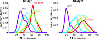
| Figure 3: Density plots for both Study 1 and Study 2 visualising the generating distribution of option values for each domain, with male and female faces plotted separately. |
First, we plotted for each participant the mean (Figure 4a), variance (Figure 4b), skewness (Figure 4c), and kurtosis (Figure 4d) of their generating distribution. Parallel independent findings were obtained for both Study 1 and Study 2. Participants and data points that were identified as outliers (see Sections S2.1 and S2.2 in the Supplementary Materials) remained excluded from the analysis. Additionally, we observed two extreme outliers for kurtosis (65.19 and 26.66), so these two participants were removed from the analysis as well (one in faces and one in holiday destinations). From Figure 4 we can observe that the domains male, female, food, and holiday destinations have robustly increasing mean values and decreasing skewness values, consistent with our visual interpretation of the densities in Figure 3.
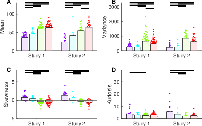
| Figure 4: Generating distribution moments plotted for each of the four domains male faces (purple), female faces (cyan), food (green), and holiday destinations (red), for Study 1 and Study 2. Black horizontal lines denote significant differences between domains at p < .05 Bonferroni-corrected for all pairs. Two outliers (kurtosis of > 25) were removed prior to analysis. |
Next, we tested whether generating distribution moments had the same or different effects on sampling rates for the optimality model and for participants. We drew our predictions from previous research on participants in economic number-based tasks ((Guan and Lee, 2018), (Baumann et al., 2020), which show greater sampling for more positively skewed (i.e., scarce) environments. We tested this hypothesis using single predictor linear regression models, each using values from one of the moments as the explanatory variable and either optimality model or participant sampling rate as the dependent variable. (Figure 5). We note that there was multicollinearity between the mean and skewness values of the distributions in both Study 1 (VIF = 3.56 and VIF = 3.83 respectively, r = –0.84) and Study 2 (VIF = 7.84 and VIF = 9.72 respectively, r = –0.92). This means that it is impossible to untangle empirically whether mean and skewness have separate effects on sampling rates. However, as multicollinearity does not affect the predictions, precision of the predictions, and the goodness-of-fit statistics, we continued with a single predictor regression analysis as detailed below. Reported p values should be interpreted with caution.
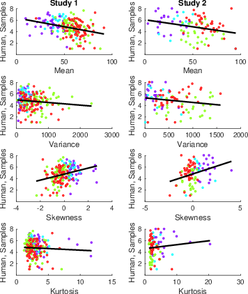
| Figure 5: Scatterplots of generating distribution moments and the mean number of samples for each participant, for Study 1 and Study 2, separated by domain: male faces (purple), female faces (cyan), food (green), and holiday destinations (red). The black line is the regression line. |
Scatterplots relating moment values to optimality model sampling rates are shown in Figure 6 and corresponding regression statistics are shown in Table 5. The results were consistent across Studies 1 and 2: Variability in each of the four moments explains optimality model sampling rates, with increased mean and variance reducing sampling rates and increased skewness and kurtosis increasing sampling rates. We then performed the same analyses, but this time relating moment values to participant sampling rates, to confirm that participants would produce some of the same effects as the optimality model. Scatterplots relating moment values to participant sampling rates are shown in Figure 5 and corresponding regression statistics are shown in (Table 6). In both studies, lower means and more positive skewness increased the sampling rate, consistent with the results of from the optimality model’s sampling rate. However, participants’ sampling rate did not show show any significant results for the moments variance or kurtosis.
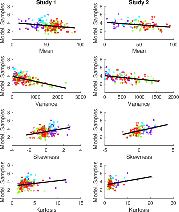
| Figure 6: Scatterplots of generating distribution moments and the mean number of samples for the optimality model, for Study 1 and Study 2, separated by domain: male faces (purple), female faces (cyan), food (green), and holiday destinations (red). The black line is the regression line. |
| Table 5: Single predictor regression analysis of the optimality model’s sampling rate and generating distribution moments. *** p < .001, ** p < .01, * p < .05. |
| Study | Moment | Coefficients | | BF10 |
| 4*Study 1 | Mean | β = –0.014, t(201) = –3.557*** | 5.9% | 42.16 |
| | Variance | β = –0.001, t(201) = –8.153*** | 24.9% | > 100 |
| | Skewness | β = 0.360, t(201) = 4.793*** | 10.3% | > 100 |
| | Kurtosis | β = 0.129, t(201) = 3.178** | 4.8% | 13.66 |
| 4*Study 2 | Mean | β = –0.012, t(94) = –3.004** | 8.8% | 10.49 |
| | Variance | β = –0.001, t(94) = –4.131*** | 15.4% | > 100 |
| | Skewness | β = 0.367, t(94) = 4.623*** | 18.5% | > 100 |
| | Kurtosis | β = 0.099, t(94) = 3.194** | 9.8% | 17.10 |
| Table 6: Single predictor regression analysis of the participants’ sampling rate and generating distribution moments. *** p < .001, ** p < .01, * p < .05. |
| Study | Moment | Coefficients | | BF10 |
| 4*Study 1 | Mean | β = –0.030, t(201) = –4.926*** | 10.8% | > 100 |
| | Variance | β = –0.0005, t(201) = –1.694 | 0.9% | 0.58 |
| | Skewness | β = 0.523, t(201) = 4.332*** | 8.5% | > 100 |
| | Kurtosis | β = –0.013, t(201) = –0.303 | 0.4% | 0.16 |
| 4*Study 2 | Mean | β = –0.024, t(94) = –2.923** | 8.3% | 8.58 |
| | Variance | β = –0.0008, t(94) = –1.761 | 2.2% | 0.84 |
| | Skewness | β = 0.542, t(94) = 3.191** | 9.8% | 16.99 |
| | Kurtosis | β = 0.068, t(94) = 1.029 | 0.1% | 0.34 |
These effects are in line with previous findings from full information problems using number-based tasks showing greater sampling in scarce environments (i.e., option generating distributions with lower means or more positive skew) (Baumann et al., 2020,Guan and Lee, 2018,Guan et al., 2014). Moreover, we find that mean and skewness values affect the sampling rate of both participants and the optimality model in the same way.
5 Discussion
The two studies described here addressed our pre-registered hypothesis, inspired by the results reported by (Furl et al., 2019), that mate choice is a special decision-making domain that provokes an oversampling bias on optimal stopping tasks, and that this oversampling bias may not be observed in other domains (e.g., food, holiday destinations). However, contrary to our a priori expectations, we replicated in both studies that oversampling generalised across three image-based decision-making domains (face, food and holiday detination attractiveness). Therefore, our results were more consistent with a second hypothesis, by which participants might oversample across many diverse image-based domains.
Specifically, we found that while different domains did not lead to qualitatively different biases (oversampling versus undersampling), sampling rates in these domains were increased for positively skewed (i.e., scarce) option generating distributions, consistent with other work using number-based full information tasks (Baumann et al., 2020). What led to this conclusion was the observation that there were modulations in sampling rate for both agents (participants and model) from domain to domain. For example, both participants and the optimality model sampled more in the faces domain, compared to the food and holiday destination domains, while the faces domain also had the lowest mean and most positively skewed generating distribution (Figures 1 and 3). As such, we suggest that the mean and skewness of the generating distribution could statistically explain variations in sampling behaviour observed for different domains. This conclusion is further supported by our finding that the optimality model’s sampling rate also correlated with the moments in a similar way as those of the participants. In other words, the moments of the generating distribution led to the same domain-related variations in sampling rates for both participants and the model.
One of the main novelties of our approach to optimal stopping problems is that participants generated their own prior distribution of subjective values of attractiveness during a phase 1 rating task. Such a methodological arrangement is advantageous for several reasons, which we describe below.
First, we can use this arrangement to study how participants’ decision strategies respond to natural variability in real-world domains. Our manipulation of decision-making domain effectively provided an experimental manipulation of distribution moments, but using moments that are representative of natural image-based domains. In contrast, artificial exogenous manipulations of price distributions, as used by previous studies (Baumann et al., 2020) may or may not produce distributions of values that resemble the corresponding real-world price distributions.
Second, in many natural domains, for example face attractiveness in mate choice (Furl et al., 2019), there simply does not exist any objective measure of the option values. Our approach can be applied to such real-world scenarios where option values, and consequently options’ ranks, can be assigned subjectively using phase 1 ratings. As more researchers investigate sampling behaviour on optimal stopping tasks using images rather than numbers, our way of specifying the mean and variance of the generating distribution might yet be the best option. After all, using only images requires the researcher to obtain the option values separately for each individual, as the value of these kind of complex, naturalistic stimuli often cannot be objectively defined (Trendl et al., 2021).
Third, our phase 1 rating task in some ways resembles real-world a priori learning of the distributions that might generate the option values for a specific decision. Many previous studies have attempted to compute optimality measures based on an approximation of participants’ perceived option generating distribution. For example, Some studies (e.g., Costa and Averbeck, 2015,Cardinale et al., 2021) assumed participants used real-world values as their generating distribution and so offered them options sampled from real-world markets to conform with participants’ presumed pre-existing prior. Other studies attempted to teach participants artificially-created generating distributions, either through verbal descriptions using statistical terminology, graphs of the probability densities of statistical distributions (Baumann et al., 2020,Lee and Courey, 2020), enriched feedback or financial rewards (Campbell and Lee, 2006), or through repeated interactions with the sequences of options (Goldstein et al., 2020). As discussed above, these kinds of learning schemes might be best-suited to research scenarios where the rank of an option within its sequence can be computed directly from the objective (numerical) values. However, these learning schemes may not always be representative of real-life distribution learning, which occurs through repeated interaction with many samples from the generating distribution, often at random, prior to the decision problem. For example, people generally learn the facial attractiveness distribution of mate choice options through their visual experience of faces. Similarly, we learn the distribution of food option values at restaurants based on our prior experience at restaurants. Neither of these naturalistic examples involves visual inspection or statistical interpretation of a probability density graph. Our procedure (i.e., experiencing distribution samples during the phase 1 rating task and when sampling options during phase 2) resembles real-world distribution learning, at least in the sense that participants learn through sequential experience of samples from the generating distribution.
Fourth, our phase 1 rating task ensures not only that participants are exposed to and have the opportunity to learn the a priori distribution that generates the option values (a defining feature of full-information problems), but also gives researchers an opportunity to programme the optimality model using participants’ personalised subjective values, which may vary from participant to participant. Here, we consider the possibility that our approach of measuring subjective option values in a separate phase might even benefit studies of domains where objectively-measurable value distributions are already available, such that of prices. This is because a participant’s subjective valuation of a stimulus such as a number (e.g., a price), may not necessarily equal the number’s objective value, as displayed on an exogenous statistical distribution provided by the researcher to a participant. For example, a participant might subjectively valuate a sizeable difference between £0 and £10 but a negligible difference between £1000 and £1010 and then act on this subjective valuation (rather than the objective price) when making decisions. This distinction would be relevant for full information problems, where the absolute option value (rather than its relative rank) is needed to solve the decision problem. Even further, the style with which participants valuate numbers or other stimuli is likely subject to individual differences (e.g., perhaps participants from different socioeconomic backgrounds evaluate the same prices differently). Methods that attempt to teach participants generating distributions using mathematical representations cannot account for such factors. In sum, participants’ subjective evaluations of prices might be differently distributed than the raw price values and, further, there might be individual differences in how participants evaluate prices. Our approach of using subjective instead of objective values when programming optimality models could account for these subjective factors. In contrast, studies that use only objectively-measured price distributions might be implementing optimality models that optimise a different quantity than participants, who instead might attempt to optimise the subjective values of their choices. However, further research will be necessary to determine how subjective and objective value distributions might differ in natural domains and which better represent the quantity that participants truly attempt to optimise when solving optimal stopping problems.
Here, we go beyond artificial experimental environments and show that natural image domains for realistic decision problems have variations in distribution shape that can affect sampling rate. Our findings also go beyond those of previous studies which have mainly focused on altering the skewness of the generating distribution and neglected to investigate other distribution moments. In fact, upon closer investigation of the distributions used by (Baumann et al., 2020) in Experiment 2 we found that the distributions did not just differ in skewness, but in mean, variance and kurtosis as well. As we found that participants’ sampling rate could be predicted by both the mean and skewness of the generating distribution, we believe that no conclusive claims can be made solely regarding the relationship between the skewness of the generating distribution and sampling behaviour.
At this point, one might speculate that there exists an unknown individual difference variable, which could dispose some individuals, who tend to evaluate options in a positively-skewed way, to sample more as well. Although as yet there is no evidence for such a disposition, and we cannot know at this time the nature or identity of such a hypothetical disposition, its discovery would have important implications for predicting real-world decisions. That is, participants’ decision patterns should be predictable from how they subjectively evaluate options. Although this explanation might be tempting, it is more likely that the link between the moments of the generating distribution and participants’ sampling rate arises because of computational mechanisms involved inherently in solving optimal stopping problems. Indeed, we found that moment values produced similar sampling effects in our optimality model (Figure 6) as they did for the participants (Figure 5), even though the model has no individual disposition to sample more or less, and merely computes the solution to the optimal stopping problem. Moreover, we observe that the relationship between sampling rate and distribution moments does not hold for participants in general, but depends on which domain a participant was assigned to. For example, the participants who sampled the most were the ones in the positively skewed male face domain (see Figure 5).
To conclude, this paper provides novel insights into human sampling behaviour by directly comparing decision biases across three image-based decision making domains. Our studies support earlier findings on the facial attractiveness task, showing that participants oversample compared to an optimality model. Results for the decision-making domains food and holiday destinations also revealed an oversampling bias in participants. Additionally, and perhaps most importantly, we found evidence that sampling biases can be predicted by the mean and skewness of the underlying distribution of domain-specific option values.
References
-
[Abdelaziz and Krichen, 2006]
-
Abdelaziz, F. B. & Krichen, S. (2006).
Optimal stopping problems by two or more decision makers: A survey.
Computational Management Science, 4(2), 89–111,
https://doi.org/10.1007/s10287-006-0029-5.
- [Anwyl-Irvine et al., 2020]
-
Anwyl-Irvine, A. L., Massonnié, J., Flitton, A., Kirkham, N., &
Evershed, J. K. (2020).
Gorilla in our midst: An online behavioral experiment builder.
Behavior Research Methods, 52(1), 388–407,
https://doi.org/10.3758/s13428-019-01237-x.
- [Backwell and Passmore, 1996]
-
Backwell, P. R. Y. & Passmore, N. I. (1996).
Time constraints and multiple choice criteria in the sampling
behaviour and mate choice of the fiddler crab, Uca annulipes.
Behavioral Ecology and Sociobiology, 38(6), 407–416,
https://doi.org/10.1007/s002650050258.
- [Baumann et al., 2020]
-
Baumann, C., Singmann, H., Gershman, S. J., & von Helversen, B. (2020).
A linear threshold model for optimal stopping behavior.
Proceedings of the National Academy of Sciences, 117(23),
12750–12755, https://doi.org/10.1073/pnas.2002312117.
- [Bearden et al., 2006]
-
Bearden, J. N., Rapoport, A., & Murphy, R. (2006).
Sequential observation and selection with rank-dependent payoffs:
An experimental study.
Management Science, 52(9), 1437–1449,
https://doi.org/10.1287/mnsc.1060.0535.
- [Blechert et al., 2019]
-
Blechert, J., Lender, A., Polk, S., Busch, N. A., & Ohla, K. (2019).
Food-Pics_Extended — An Image Database for
Experimental Research on Eating and Appetite: Additional
Images, Normative Ratings and an Updated Review.
Frontiers in Psychology, 10, 307,
https://doi.org/10.3389/fpsyg.2019.00307.
- [Campbell and Lee, 2006]
-
Campbell, J. & Lee, M. D. (2006).
The Effect of Feedback and Financial Reward on Human
Performance Solving ‘Secretary’ Problems.
Proceedings of the Annual Meeting of the Cognitive Science
Society, 28(28).
- [Cardinale et al., 2021]
-
Cardinale, E. M., et al. (2021).
Deliberative Choice Strategies in Youths: Relevance to
Transdiagnostic Anxiety Symptoms.
Clinical Psychological Science, (pp. 1–11).,
https://doi.org/10.1177/2167702621991805.
- [Costa and Averbeck, 2015]
-
Costa, V. D. & Averbeck, B. B. (2015).
Frontal-Parietal and Limbic-Striatal Activity Underlies
Information Sampling in the Best Choice Problem.
Cerebral Cortex, 25(4), 972–982,
https://doi.org/10.1093/cercor/bht286.
- [Ferguson, 1989]
-
Ferguson, T. S. (1989).
Who Solved the Secretary Problem?
Statistical Science, 4(3), 282–289,
https://doi.org/10.1214/ss/1177012493.
- [Freeman, 1983]
-
Freeman, P. R. (1983).
The Secretary Problem and Its Extensions: A Review.
International Statistical Review / Revue Internationale de
Statistique, 51(2), 189–206, https://doi.org/10.2307/1402748.
- [Furl and Averbeck, 2011]
-
Furl, N. & Averbeck, B. B. (2011).
Parietal Cortex and Insula Relate to Evidence Seeking
Relevant to Reward-Related Decisions.
Journal of Neuroscience, 31(48), 17572–17582,
https://doi.org/10.1523/JNEUROSCI.4236-11.2011.
- [Furl et al., 2019]
-
Furl, N., Averbeck, B. B., & McKay, R. T. (2019).
Looking for Mr(s) Right: Decision bias can prevent us
from finding the most attractive face.
Cognitive psychology, 111, 1–14,
https://doi.org/10.1016/j.cogpsych.2019.02.002.
- [Gilbert and Mosteller, 1966]
-
Gilbert, J. P. & Mosteller, F. (1966).
Recognizing the Maximum of a Sequence.
Journal of the American Statistical Association, 61(313),
35–73, https://doi.org/10.2307/2283044.
- [Goldstein et al., 2020]
-
Goldstein, D. G., McAfee, R. P., Suri, S., & Wright, J. R. (2020).
Learning When to Stop Searching.
Management Science, 66(3), 1375–1394,
https://doi.org/10.1287/mnsc.2018.3245.
- [Guan and Lee, 2018]
-
Guan, M. & Lee, M. D. (2018).
The effect of goals and environments on human performance in optimal
stopping problems.
Decision, 5(4), 339–361,
https://doi.org/10.1037/dec0000081.
- [Guan et al., 2014]
-
Guan, M., Lee, M. D., & Silva, A. (2014).
Threshold Models of Human Decision Making on Optimal
Stopping Problems in Different Environments.
Proceedings of the Annual Meeting of the Cognitive Science
Society, 36(36).
- [Guan et al., 2020]
-
Guan, M., Stokes, R., Vandekerckhove, J., & Lee, M. D. (2020).
A cognitive modeling analysis of risk in sequential choice tasks.
Judgment and Decision Making, 15, 823–850.
- [Hauser et al., 2017]
-
Hauser, T. U., Moutoussis, M., Dayan, P., & Dolan, R. J. (2017).
Increased decision thresholds trigger extended information gathering
across the compulsivity spectrum.
Translational Psychiatry, 7(12), 1–10,
https://doi.org/10.1038/s41398-017-0040-3.
- [Hauser et al., 2018]
-
Hauser, T. U., Moutoussis, M., Purg, N., Dayan, P., & Dolan, R. J. (2018).
Beta-Blocker Propranolol Modulates Decision Urgency During
Sequential Information Gathering.
The Journal of Neuroscience, 38(32), 7170–7178,
https://doi.org/10.1523/JNEUROSCI.0192-18.2018.
- [Hill, 2009]
-
Hill, T. P. (2009).
Knowing When to Stop: How to gamble if you
must—the mathematics of optimal stopping.
American Scientist, 97(2), 126–133.
- [Ivy and Sakaluk, 2007]
-
Ivy, T. M. & Sakaluk, S. K. (2007).
Sequential mate choice in decorated crickets: Females use a fixed
internal threshold in pre- and postcopulatory choice.
Animal Behaviour, 74(4), 1065–1072,
https://doi.org/10.1016/j.anbehav.2007.01.017.
- [Kahan et al., 1967]
-
Kahan, J. P., Rapoport, A., & Jones, L. V. (1967).
Decision making in a sequential search task.
Perception & Psychophysics, 2(8), 374–376,
https://doi.org/10.3758/BF03210074.
- [Lee, 2006]
-
Lee, M. D. (2006).
A Hierarchical Bayesian Model of Human Decision-Making on
an Optimal Stopping Problem.
Cognitive Science, 30(3), 1–26,
https://doi.org/10.1207/s15516709cog0000_69.
- [Lee and Courey, 2020]
-
Lee, M. D. & Courey, K. A. (2020).
Modeling Optimal Stopping in Changing Environments: A Case
Study in Mate Selection.
Computational Brain & Behavior, 4(1), 1–17,
https://doi.org/10.1007/s42113-020-00085-9.
- [Lee and Wagenmakers, 2013]
-
Lee, M. D. & Wagenmakers, E.-J. (2013).
Bayesian cognitive modeling: A practical course.
New York, NY, US: Cambridge University Press.
- [Matejka et al., 2016]
-
Matejka, J., Glueck, M., Grossman, T., & Fitzmaurice, G. (2016).
The Effect of Visual Appearance on the Performance of
Continuous Sliders and Visual Analogue Scales.
Proceedings of the 2016 CHI Conference on Human Factors in
Computing Systems, (pp. 5421–5432).,
https://doi.org/10.1145/2858036.2858063.
- [MATLAB, 2015]
-
MATLAB (2015).
Version 2015b.
The MathWorks Inc.
- [Milinski and Bakker, 1992]
-
Milinski, M. & Bakker, T. (1992).
Costs influences sequential mate choice in sticklebacks, gasterosteus
aculeatus.
Proceedings of the Royal Society of London. Series B: Biological
Sciences, 250(1329), 229–233,
https://doi.org/10.1098/rspb.1992.0153.
- [Morey and Rouder, 2018]
-
Morey, R. D. & Rouder, J. N. (2018).
BayesFactor: Computation of Bayes Factors for Common
Designs.
- [Prolific, 2014]
-
Prolific (2014).
Available at: https://www.prolific.co.
Prolific.
- [RStudioTeam, 2020]
-
RStudioTeam (2020).
RStudio: Integrated Development Environment for R.
RStudio, PBC.
- [Seale and Rapoport, 1997]
-
Seale, D. A. & Rapoport, A. (1997).
Sequential Decision Making with Relative Ranks: An
Experimental Investigation of the "Secretary Problem".
Organizational Behavior and Human Decision Processes, 69(3), 221–236, https://doi.org/10.1006/obhd.1997.2683.
- [Shapira and Venezia, 1981]
-
Shapira, Z. & Venezia, I. (1981).
Optional stopping on nonstationary series.
Organizational Behavior and Human Performance, 27(1),
32–49, https://doi.org/10.1016/0030-5073(81)90037-4.
- [Shu, 2008]
-
Shu, S. B. (2008).
Future-biased search: The quest for the ideal.
Journal of Behavioral Decision Making, 21(4), 352–377,
https://doi.org/10.1002/bdm.593.
- [Taber, 2018]
-
Taber, K. S. (2018).
The Use of Cronbach’s Alpha When Developing and
Reporting Research Instruments in Science Education.
Research in Science Education, 48(6), 1273–1296,
https://doi.org/10.1007/s11165-016-9602-2.
- [Trendl et al., 2021]
-
Trendl, A., Stewart, N., & Mullett, T. L. (2021).
A zero attraction effect in naturalistic choice.
Decision, 8(1), 55,
https://doi.org/10.1037/dec0000145.
- [Van der Leer et al., 2015]
-
Van der Leer, L., Hartig, B., Goldmanis, M., & McKay, R. (2015).
Delusion proneness and ‘jumping to conclusions’: Relative and
absolute effects.
Psychological Medicine, 45(6), 1253–1262,
https://doi.org/10.1017/S0033291714002359.
- [Wagenmakers et al., 2018]
-
Wagenmakers, E.-J., et al. (2018).
Bayesian inference for psychology. Part II: Example
applications with JASP.
Psychonomic Bulletin & Review, 25(1), 58–76,
https://doi.org/10.3758/s13423-017-1323-7.
- [Zwick et al., 2003]
-
Zwick, R., Rapoport, A., Lo, A. K. C., & Muthukrishnan, A. V. (2003).
Consumer Sequential Search: Not Enough or Too Much?
Marketing Science, 22(4), 503–519,
https://doi.org/10.1287/mksc.22.4.503.24909.
Supplementary Materials
S1 Filenames corresponding to food images
0001, 0002, 0004, 0007, 0009, 0010, 0016, 0022 ,0025, 0032, 0044, 0049, 0053, 0054, 0057, 0061, 0072, 0080, 0089, 0095, 0101, 0104, 0110, 0113, 0123, 0143, 0145, 0150, 0153, 0157, 0166, 0167, 0175, 0176, 0192, 0194, 0198, 0199, 0200, 0201, 0206, 0222, 0227, 0233, 0244, 0248, 0249, 0250, 0251, 0255, 0256, 0258, 0259, 0269, 0278, 0279, 0280, 0281, 0282, 0283, 0285, 0298, 0311, 0313, 0317, 0319, 0321, 0323, 0338, 0347, 0350, 0375, 0434, 0491, 0507, 0512, 0557, 0563, 0567, 0569, 0581, 0602, 0631, 0654, 0662, 0741, 0770, 0810, 0894, 0896
S2 Attention check Study 1
We decided to add an attention check to phase one of Study 1 to compensate for the unsupervised nature of online data collection. Each attention check comprised two screens that were shown one after the other. Attention checks showed up at nine random points (5% of the total of 180 images) throughout phase one. This totals 18 attention checks (nine time points x two screens). Each attention check screen showed a cross (either black or red), a ‘next’ button, and the text “press ‘next’ when the cross disappears”. The cross disappeared at a random time interval between one and five seconds. The ‘next’ button was active the whole time. Reaction times for pressing the ‘next’ button were recorded for both screens, that is, for both the black and the red cross. Before data analysis, participants’ response time for pressing the ‘next’ button was compared to the actual time interval before the cross disappeared (cross display time). If participants were paying attention, they would not press the ‘next’ button as soon as it appeared, but would instead read the text and respond only after the cross had disappeared. Thus, if participants’ response time exceeded the cross display time, they passed the attention check.
S2.1 Outlier removal Study 1
Although restrictions were set in Prolific to collect only 75 participants per domain, upon inspection of the data, we discovered that 76 participants were recruited in the food domain. As no duplicate IDs were found, we included all 76 participants in the data analysis. Also of note is that one participant’s self-reported age was 16 (faces domain) and one participant’s self-reported age was 36 (food domain), despite the enrolment restrictions set beforehand on Prolific. Considering that neither age required ethical reconsideration under British Psychological Society guidelines, we decided to include both participants in the analyses. To control for task incongruent behaviour, we preregistered that all data points (i.e., mean number of samples and mean rank for each participant) had to be within 2.5 SD of each condition mean. We found three data points violating this assumption: one in the faces domain (in the rank of the chosen face), and two in the food domain (in the number of samples). These data points were thus excluded from the data analysis. If participants failed > 25% of the attention checks (i.e., more than five) they were also excluded from the data analysis. Using this measure, another 18 participants were excluded (seven in the faces domain, four in the food domain, and seven in the holiday destinations domain).
S2.2 Outlier removal Study 2
One data point in the faces domain, for the mean number of samples, was excluded because it was > 2.5 SD from the condition mean.
| Table S1: Demographic statistics for each of the three domains: faces, food and holiday destinations. *One participant did not provide a valid response to this demographics question. |
| | Faces | Food | Holiday Destinations | |
| | (N = 68) | (N = 72) | (N = 68) | |
| Age | | | | |
| Mean (SD) | 26.43 (4.869) | 25.53 (5.259) | 27.13 (4.597) | |
| Missing* | 1 | 0 | 0 | |
| Sex | | | | |
| Male | 25 | 28 | 24 | |
| Female | 42 | 43 | 43 | |
| Other | 1 | 1 | 1 | |
| Nationality | | | | |
| United Kingdom | 34 | 44 | 54 | |
| Ireland | 0 | 6 | 1 | |
| United States | 14 | 11 | 7 | |
| Canada | 19 | 11 | 3 | |
| Australia | 0 | 0 | 3 | |
| New Zealand | 1 | 0 | 0 | |
| Table S2: Demographic statistics for Study 2, for each of the three domains: faces, food and holiday destinations. |
| | Faces | Food | Holiday Destinations | |
| | (N = 32) | (N = 28) | (N = 36) | |
| Age | | | | |
| Mean (SD) | 28.13 (14.89) | 35.68 (18.23) | 28.22 (15.71) | |
| Sex | | | | |
| Male | 5 | 11 | 10 | |
| Female | 26 | 17 | 26 | |
| Other | 1 | 0 | 0 | |
This document was translated from LATEX by
HEVEA.