Judgment and Decision Making, Vol. ‍17, No. ‍2, March 2022, pp. 400-424

Abstract: Humans are evidently able to learn contingencies from the co-occurrence of cues and outcomes. But how do humans judge contingencies when observations of cue and outcome are learned on different occasions? The pseudocontingency framework proposes that humans rely on base-rate correlations across contexts, that is, whether outcome base rates increase or decrease with cue base rates. Here, we elaborate on an alternative mechanism for pseudocontingencies that exploits base rate information within contexts. In two experiments, cue and outcome base rates varied across four contexts, but the correlation by base rates was kept constant at zero. In some contexts, cue and outcome base rates were aligned (e.g., cue and outcome base rates were both high). In other contexts, cue and outcome base rates were misaligned (e.g., cue base rate was high, but outcome base rate was low). Judged contingencies were more positive for contexts in which cue and outcome base rates were aligned than in contexts in which cue and outcome base rates were misaligned. Our findings indicate that people use the alignment of base rates to infer contingencies conditional on the context. As such, they lend support to the pseudocontingency framework, which predicts that decision makers rely on base rates to approximate contingencies. However, they challenge previous conceptions of pseudocontingencies as a uniform inference from correlated base rates. Instead, they suggest that people possess a repertoire of multiple contingency inferences that differ with regard to informational requirements and areas of applicability.

Keywords: base rates, contingency learning, ecological correlation, probability judgment, pseudocontingencies

1 Introduction

Contingency detection is an intriguing capacity, essential for understanding the past and predicting the future (Crocker, 1981). Accordingly, a plethora of empirical studies has elaborated on this ability to detect contingencies between two binary events (e.g., Allan, 1993; De Houwer & Beckers, 2002; Mata, 2016). In a typical contingency learning experiment, participants are exposed to joint observations of a binary cue and a binary outcome variable. For instance, participants observe a series of patient data consisting of treatment information on the one hand (i.e., whether a patient received Vaccine X or Y) and outcome information on the other (i.e., whether a patient’s health improved or deteriorated). Here, the contingency could be calculated from the frequencies of a 2×2 table resulting from the combination of the cue and outcome levels. Specifically, it can be calculated as the difference between the conditional probability of improved (vs. deteriorated) health given Treatment X and the conditional probability of improved (vs. deteriorated) health given Treatment Y, Δ p = (p(healthy | treatment X) – (p(healthy | treatment Y), (Jenkins & Ward, 1965). Ample evidence suggests that humans are capable of estimating such contingencies with high accuracy (for reviews, see Allan, 1993; Hattori & Oaksford, 2007).¹

1.1 Contingency learning from aggregated and grouped observations

Unfortunately, learners do not always find themselves faced with conditions that are conducive to learning, providing them with the necessary information on joint observations, that is, the combinations of cue and outcome. Instead, observations are often aggregated across individuals or separated in time (Fiedler et al., 2009). For instance, a nurse may observe whether patients are treated with Vaccine X or Y on one day, but may observe whether patients got better or worse on another. Thus, without external memory aids, it can be challenging to connect cues and outcomes. Or, a reader of a newspaper may receive aggregated information only: the proportion of patients treated with Vaccine X and the proportion of patients suffering from severe symptoms. In that case, it is actually impossible to connect cue and outcome values. Nevertheless, contingency judgments are still crucial to understanding one’s environment, so how do individuals arrive at contingency judgments in the absence of paired observations?

Fiedler and Freytag (2004) proposed that people rely on the univariate base rates of cue and outcome to infer a contingency. In one of their seminal studies, participants observed information about certain individuals’ test results as cue values (e.g., X vs. Y) in two contexts (target group: blue vs. green). In the blue group, X was more prevalent, while in the green group, Y was more prevalent. On a later occasion, participants observed information about outcomes, either positive or negative. In the blue group, positive outcomes were more frequent, while in the green group, negative outcomes dominated. Crucially, participants inferred a positive contingency between Cue X and the positive outcome in both contexts, although the actual contingency was negative (Exp. 3 in Fiedler & Freytag, 2004). This inference of a contingency from correlated base rates – referred to as pseudocontingency – has been demonstrated in various studies where cue and outcomes were learned on different occasions, but also if they were learned simultaneously (for reviews, see Fiedler et al., 2009; Fiedler et al., 2013).

While this research clearly shows the reliance on cue and outcome base rates in contingency judgment, it leaves open the question whether participants tend to infer the contingencies conditional on the context or based on the unconditional contingency. Applied to the example above, it is thus far unknown whether participants judged the contingency based on the cue-outcome relation separately within the blue group and within the green group (i.e., conditional on the context variable group) or based on the cue-outcome relation collapsed across groups (unconditional). As we will elaborate in the next section, the answer to this question will also shed light on the rule behind contingency inferences from base rates.

1.2 Pseudocontingencies: contingency inferences from base rates

To explain more precisely what is at issue, it is helpful to first elaborate on the standard conceptualization of pseudocontingencies as a cognitive analog to so-called ecological correlations (Robinson, 1950). In Robinson’s original terminology, an ecological correlation refers to a correlation between two variables’ base rates across different contexts (e.g., cue and outcome base rates are correlated across contexts). As Robinson demonstrated, the ecological correlation can diverge drastically from the contingency at the individuating level. For an illustration, consider the 2×2 tables for cues and outcomes across two contexts displayed in Figure 1a. As shown in that figure, there are two contexts, represented by two different diseases (Diseases A and B). The cue base rate (i.e., base rate of Therapy X) is low for Disease A, p(Therapy X|A) = .25, and so is the outcome base rate, p(healthy|A) = .25. For Disease B, however, cue base rate and outcome base rate are both high, p(Therapy X|B) = p(healthy|B) = .75. In other words, cue and outcome base rates are correlated across contexts. The higher the cue base rate, the higher the outcome base rate, yielding a positive ecological correlation. At the same time, the contingency between cue and outcome within each context is negative, Δ p = −.33. And the unconditional contingency – collapsed across contexts – is zero, Δ p = .0. However, experimental studies using this distribution (or similar ones) consistently reveal that participants perceive a positive contingency between cue and outcome (e.g., Bott & Meiser, 2020; Fiedler & Freytag, 2004; Fleig et al., 2017; Meiser & Hewstone, 2004; Meiser et al., 2018; Vogel, Freytag, et al., 2013).

---

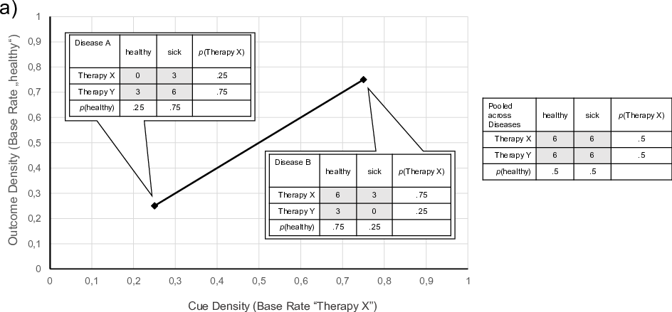
Figure 1: Ecological correlations by cue and outcome base rates across contexts. In Figure 1a, the base rate of the outcome “healthy” increases with the base rate of the cue “Therapy X” across contexts, here diseases. Thus, the ecological correlation (solid line) is positive, r = +1.0. The conditional contingency between Therapy X and outcome “healthy” within each context, however, is negative both in Context A, Δ p|A = 0/3 – 6/9 = –.33, and in Context B, Δ p|B = 6/9 – 3/3 = –.33. 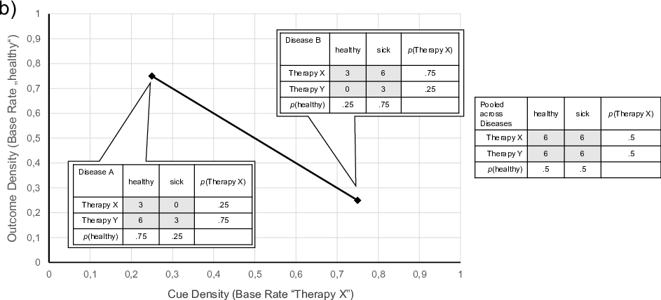In Figure 1b, the ecological correlation (solid line) is negative, r = –1.0. Here, the conditional contingency is positive in Context A, Δ p|A = 3/3 – 6/9 = +.33, as well as in Context B, Δ p|B = 3/9 – 0/3 = +.33. The unconditional contingency calculated from the pooled frequencies (right table) is zero, Δ p = 6/12 – 6/12 = .0, in Figure 1a and 1b.

---

Now, consider Figure 1b. Here, the cue base rate is low for Disease A, p(Therapy X|A) = .25, but the outcome base rate is high, p(healthy|A) = .75. In contrast, for Disease B, the cue base rate is high, p(Therapy X|B) = .75, but the outcome base rate is low, p(healthy|B) = .25.

Thus, across contexts, an increase in the cue base rate is associated with a decrease in the outcome base rate, which is equivalent to a negative ecological correlation. Though the actual contingency within each context is positive now, Δ p = +.33, and the unconditional contingency is zero, Δ p = .0, people tend to infer a negative contingency between cue and outcome. Therefore, several authors proposed that people use the ecological correlation across contexts to infer the contingency between cue and outcome (e.g., Fiedler & Freytag, 2004; Vogel, Kutzner, et al., 2013).

However, there is an alternative to this explanation. As is obvious from the tables in Figure 1a, the positive ecological correlation coincides with an alignment of skewed base rates within ecologies. The base rates of cue and outcome are both low, p(Therapy X|A) < .5; p(healthy|A) < .5, or both high, p(Therapy X|B) > .5; p(healthy|B) > .5. In contrast, in Figure 1b, the negative ecological correlation is due to the fact that base rates in all contexts are misaligned. Thus, a low cue base rate, p(Therapy X|A) < .5, coincides with a high outcome base rate, p(healthy|A) > .5., and vice versa, p(Therapy X|B) > .5; p(healthy|B) < .5. In other words, the alignment or misalignment of base rates within contexts displayed in Figures 1a and 1b entails the ecological correlation. Thus, based on the present state of the literature, it is impossible to discern the effect of the base rate information within each context from the ecological correlation, which is defined across contexts.

Pertinent to the present research, the critical role of aligned base rates in contingency detection has been discussed previously (Fiedler & Freytag, 2004; Kutzner, 2009; Vogel & Kutzner, 2017), with Kutzner et al. (2011a, p. 212) proposing that pseudocontingencies “imply a positive contingency when the base rates of the target variables are skewed in the same direction and a negative contingency when the base rates are skewed in opposite directions.” Indeed, research studying contingency judgments in single-context paradigms supports this notion. For instance, Vogel and Kutzner (2017) presented participants with stated base rates of cues (Brand: X vs. Y) and outcomes (customer satisfaction: low vs. high) and found that participants perceived a positive contingency between Brand X and customer satisfaction if base rates of Brand X and customer satisfaction were both high or both low. Instead, a negative contingency was inferred if the cue base rate mismatched the outcome base rate, for instance, if Brand X was more prevalent than Brand Y, but fewer customers were satisfied than dissatisfied. Together, these findings clearly attest to the effect of base rate alignment on contingency judgments, at least if bivariate observations of cue and outcome are impossible (also see Blanco et al., 2013; Eder et al., 2011; Ernst et al., 2019; Fiedler, 2010; for demonstrations of base-rate effects in paradigms with joint cue- and outcome observations).

Though findings from single-context paradigms suggest that aligned base rates are the driving force behind pseudocontingencies, there is an alternative to this interpretation. As Fiedler et al. (2007) pointed out, those findings may reflect an implicit ecological correlation (see also Fiedler et al., 2009; Vogel, Kutzner, et al., 2013). That is, in the absence of an observable ecological correlation, people would use the alignment of base rates (e.g., high cue and high outcome base rate) to infer an ecological correlation, which in turn would drive biased contingency estimates. This conjecture, however, has not yet been put to the test.

Hence, there are two crucial implications: First, the alignment of base rates within contexts might be sufficient to drive the pseudocontingency inference – independent of the ecological correlation. Second, pseudocontingencies might actually reflect conditional contingency inferences within each context. In this vein, the context variable might therefore serve as a moderator of contingency judgments if the alignment of base rates varies between contexts.

1.3 Present research

The present research aims at testing the impact of aligned base rates on contingency judgments. A straightforward test of the role of base rate alignment over and above ecological correlations can be achieved by varying the base rate alignment while keeping the observable ecological correlation constant at zero. Moreover, we pit predictions from base-rate alignment against predictions from actual contingency learning.

1.3.1 Cue and outcome base rate within contexts

We conducted two experiments where participants were exposed to cue and outcome information across four contexts. As our central manipulation, we varied the alignment of base rates across the four contexts by using an orthogonal within-participant variation of cue and outcome base rate (detailed in Table 1). To isolate the effect of base rate alignment from the ecological correlation, the ecological correlation was held constant at zero. Moreover, the unconditional contingency was also kept constant at zero to isolate the effect of aligned base rates from previously shown illusions resulting from a Simpson Paradox (Simpson, 1951).² Thus, if participants used the ecological correlation or the unconditional contingencies to infer conditional contingencies, no systematic differences should be found between contexts. To pit predictions against actual learning of conditional contingencies, the alignment of base rates always implied a positive contingency in contexts in which the actual contingency was negative (Contexts A & D), and vice versa, a negative contingency in contexts in which the actual contingency was positive (Contexts B & C). We hypothesize that participants’ inferred contingency estimates are driven by the implication of the alignment of base rates, resulting in different contingency estimates as a function of the context. Concretely, we predict that participants will infer more positive contingencies for contexts where cue and outcome base rates are aligned (both low or both high) than for contexts where they are misaligned (cue base rate is low, but outcome base rate is high, or vice versa).

---

Table 1: Stimulus distributions for cues and outcomes across contexts A, B, C, & D.

	Context				Pooled
	A (HC,HO)	B (HC,LO)	C (LC,HO)	D (LC,LO)	A+B+C+D
Cell Frequencies
X+	6	3	3	0	12
X−	3	6	0	3	12
Y+	3	0	6	3	12
Y−	0	3	3	6	12
Cue Base rate
p(X)	.75	.75	.25	.25	.5
p(Y) = 1–p(X)	.25	.25	.75	.75	.5
Outcome Base rate
p(+)	.75	.25	.75	.25	.5
p(−) = 1 – p(+)	.25	.75	.25	.75	.5
Conditional Probabilities
p(+|X)	.67	.33	1.0	.0	.5
p(+|Y)	1.0	.0	.67	.33	.5
Stimulus Contingency
Δ p	−.33	+.33	+.33	−.33	.0
Note. Stimulus distribution for four contexts, A, B, C, and D. In Context A (first column), Cue X co-occurred six times with the positive outcome (X+), three times with the negative outcome (X-), etc. With a high cue base rate (HC) and high outcome base rate (HO), base rates were aligned in Context A, which implies a positive pseudocontingency between X and +. As noted in the lower row, the actual contingency between X and + in Context A was negative. In Context D, base rates were aligned due to the low cue base rate (LC) and the low outcome base rate (LO), also implying a positive pseudocontingency, despite a negative stimulus contingency. In Contexts B and C, base rates were misaligned though actual contingencies were positive.

---

H1: Perceived contingencies will be more positive in contexts in which cue and outcome base rates are aligned than in contexts in which they are misaligned.

2 Experiment 1

The first experiment sought to test whether people infer conditional contingencies and, thus, different cue-outcome relations depending on the context. We predicted that the perceived contingency between cue (e.g., Treatment X vs. Treatment Y) and outcome (e.g., improved vs. deteriorated health) depends on the alignment of predictor and outcome base rates within a given context. To differentiate between pseudocontingencies and other mechanisms that rest on the observation of joint observations of cue and outcome (e.g., Hamilton & Gifford, 1976; Rescorla & Wagner, 1972), the possibility of joint observations was precluded by block-wise presentation of cues and outcomes on different occasions (Fiedler & Freytag, 2004; Vogel & Kutzner, 2017).

2.1 Method

2.1.1 Design and participants

The design was a 2(cue base rate: low vs. high) × 2(outcome base rate: low vs. high) design, with both factors varied within participants. A power analysis using G*Power (Faul et al., 2007) revealed a required sample size of N = 34 to detect significant effects, p < .05, of moderate-size, f ≥ .25, with a probability of 1–β = .8. To compensate for potential drop-outs, a total of fifty participants (M_age = 34.14, SD = 13.59; 25 female; 24 male; 1 other) were acquired via a commercial panel (Prolific Academic) and took part for a compensation of £1 (£7.50/h).

2.1.2 Materials and procedure

The whole materials were administered online and in English using the SoSci-Survey tool (Leiner, 2014). A cover story asked participants to observe a series of patient data on different diseases, medical treatments, and symptoms. In total, there were four diseases (i.e., Morbus Alpha, Morbus Beta, Morbus Gamma, and Morbus Delta) that served as our contexts. In a first phase, participants were presented with information about the medical treatments. Starting with the first context, Morbus Alpha, participants saw a list consisting of twelve patients’ IDs (e.g., XHHOI3798V or VNVIG6689S) and which medication each of them received (”Medicine X” or “Medicine Y”). The presentation then continued with the next context, and participants were presented with a list of twelve patients suffering from Morbus Beta, with the list detailing each patient’s ID and whether they were being treated with Treatment X or Y, and so on. After the four contexts, participants entered the second phase, in which they were presented with the therapy outcomes. Specifically, they saw a list of the same Morbus Alpha patients, but now each patient ID was accompanied by the information of their health outcome, that is, whether the patient’s health improved or deteriorated (e.g., XHHOI3798V got better; VNVIG6689S got worse). The presentation then continued with the presentation of outcomes for the remaining three diseases.

We used the distribution shown in Table 1 as a manipulation of base rates. That is, for half of the diseases, the base rate of Treatment X (vs. Y) was high, p = .75, but for the other half of the diseases, the base rate of Treatment X (vs. Y) was low, p = .25. Orthogonally, the base rate of desirable outcomes (i.e., improved health) was high, p = .75, for half of the diseases, but low, p = .25, for the other. The order was held constant, so contexts always started with Morbus Alpha and ended with Morbus Delta. Yet, stimulus distributions resulting from the orthogonal manipulation for cue and outcome base rate were assigned to the diseases via a Latin square design (e.g., in Table 1, A, B, C, D vs. B, C, D, A etc.). After the presentation of therapy outcomes, participants proceeded to a manipulation check that assessed whether the base-rate manipulation was effective. For each disease, participants were to estimate the percentage of Treatment X (vs. Y) and the percentage of patients whose health had improved after the therapy. Then, participants were directed to the judgment phase. For each disease, participants were asked to indicate the probability that a positive versus a negative outcome would be observed given a patient was treated with X, or treated with Y, respectively. For instance, they read “What will happen if Medicine X is given to a patient with Morbus Alpha?” and then moved a 100-point slide bar with endpoints labelled “The patient’s condition will most likely get worse” (coded 0) and “The patient’s condition will most likely get better” (coded 1). Accordingly, the next item read “What will happen if Medicine Y is given to a patient with Morbus Alpha?”, using the same anchors. The difference between these two estimates was calculated to obtain context-wise contingency estimates serving as our dependent measure, Δ p. Finally, participants reported their demographics, were thanked, and debriefed.

2.2 Results and discussion

2.2.1 Manipulation check

Base-rate estimates for the cues (i.e., Treatment X vs. Y) were subjected to a 2(cue base rate: low vs. high) × 2(outcome base rate: low vs. high) analysis of variance (ANOVA) for repeated measures with the afex package in R (Singmann et al., 2020). To facilitate the interpretation of evidence in favor of the alternative over the null hypothesis, we calculated Bayes Factors from a Bayesian ANOVA conducted in the BayesFactor package with default priors (Morey & Rouder, 2018). A significant effect of cue base rate emerged (F(1, 49) = 42.28, p < .001, η ²_pt = .46, BF₁₀ > 1000). High base rates of Treatment X (vs. Y) yielded estimates with a mean of M = 62.6, SE = 2.54, whereas low base rates of Treatment X (vs. Y) yielded estimates with a mean of M = 34.50, SE = 2.43, indicating that the manipulation was successful and attesting to that participants learned cue base rates effectively. The effects of outcome base rate and the interaction were not significant (Fs < 1, BF₁₀s < 0.21).

Next, outcome base rates were subjected to an analogous ANOVA. This time, we observed a significant effect of the outcome base rate manipulation (F(1, 49) = 41.78, p < .001, η ²_pt = .46, BF₁₀ > 1000) with higher estimates when stimulus base rates for the desirable outcome were high (M = 62.46, SE = 2.56) rather than low (M = 36.00, SE = 2.63). The effect of cue base rate was not significant (F(1, 49) = 1.49, p = .228, η ²_pt = .03, BF₁₀ = 0.20), nor was the interaction (F(1, 49) = 0.09, p = .765, η ²_pt = .00, BF₁₀ = 0.21). Thus, participants also recognized the skew of outcome base rates.

2.2.2 Main analysis

To test our hypothesis, context-wise contingency estimates were subjected to the same type of ANOVA. The main effect of cue base rate fell short of conventional levels of significance (F(1, 49) = 3.17, p = .081, η ²_pt = .06, BF₁₀ = 0.76). The effect of outcome base rate was not significant either (F(1, 49) = 1.68, p = .201, η ²_pt = .03, BF₁₀ = 0.26). Crucially, the predicted two-way interaction was significant (F(1, 49) = 8.75, p = .005, η ²_pt = .15, BF₁₀ = 188.85), lending extreme support to Hypothesis 1 over the null hypothesis according to current conventions (Lee & Wagenmakers, 2013). For contexts with aligned base rates of cue and outcome, perceived contingencies were more positive (M_{hi cue | hi out} = .12, SE = .07; M_{low cue | low out} = .18, SE = .07), than for contexts where predictor and outcome base rates were misaligned (M_{hi cue | low out} = −.24, SE = .07; M_{low cue | hi out} = −.02, SE = .08; see Figure 2).

---

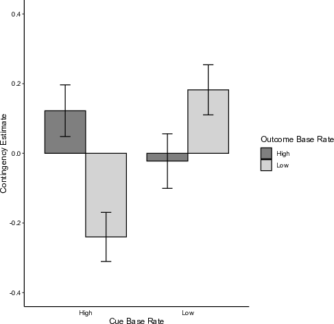
Figure 2: Results from Experiment 1. Estimates for contingency between cue (“Therapy X”) and outcome (“improved health”) as a function of cue and outcome base rates. Error bars represent +/- 1 standard error.

---

As is evident from the first study, people consider the context and infer conditional contingencies between cue and outcomes. In support of our predictions, the contingency inferences are systematic. That is, perceived contingencies were more positive for contexts in which base rates were aligned than in contexts in which base rates mismatched. This effect was observed although the actual contingencies within contexts pointed in the opposite direction, yielding a contingency illusion. However, this first experiment used a scenario that had not been established in previous research on pseudocontingencies. In fact, the scenario implied a causal relation between cue and outcome (i.e., a change in health status after an intervention). Thus, this surplus meaning might have supported the inference of cue-outcome contingencies though it is not a theoretical requirement for pseudocontingencies to occur. To test for the robustness of the results, we replicated the effect in a scenario already used in previous research on pseudocontingencies.

3 Experiment 2

The next experiment aimed at a conceptual replication of Experiment 1. Specifically, we used the same stimulus distribution as in the previous study, but adopted an established politics scenario, in which participants were asked to compare two politicians based on their answers to a politics survey (Vogel, Freytag, et al., 2013, Experiment 3). Unlike the previous study, this scenario did not imply that the cue is the cause of the outcome.

3.1 Method

3.1.1 Design and participants

Based on the same power analysis as for Experiment 1, fifty-five students (M_age = 22.17, SD = 5.90; 45 female, 9 male) from the University of Mannheim took part in an online study in exchange for course credit. The design was a 2(cue base rate: low vs. high) x 2(outcome base rate: low vs. high) within-participants design. Due to missing values on the dependent measures, one participant was removed from the data set leaving a sample of N = 54 valid cases.

3.1.2 Materials and procedure

The cover story was that two politicians, X and Y, had both responded to a politics survey. Participants were to compare those two politicians based on their answers to a survey covering four policy domains: education, environmental, migration, and internal security. In a first phase, participants were asked to study how Politician X had responded to the survey. They were presented with twelve statements from a first, randomly selected domain (e.g., internal security: “Airport controls need to be tightened.”). For each statement they saw whether Politician X had responded with “yes” or “no”. The presentation then continued with the next domain until all domains were covered. After the presentation of Politician X’s responses, participants were informed that another Politician, Y, had responded to the same survey and participants were asked to study those answers, too. After the presentation of both politicians’ survey answers for all domains, they were asked to indicate the base rates of “yes”-responses for Politician X and Politician Y in each domain. After that, the contingency estimates were assessed following a format similar to the one used in Experiment 1. Specifically, participants provided two estimates per domain. For example, they read “For a statement on internal security which Politician X answers with yes, Politician Y would probably answer with …” and were asked to provide their estimate by moving a slider on a 100-point scale with anchors ranging from “definitely no” to “ definitely yes”. Below, they provided the same statement conditional on that Politician X had answered with “no” (“For a statement on internal security that Politician X answers with no, Politician Y would probably answer with …”), using the same anchors from “definitely no” to “definitely yes”. The latter score was subtracted from the former, and then rescaled to obtain domain-wise contingency indices, Δ p, with a theoretical range from −1 to +1. Lastly, participants indicated demographic information before they were thanked and debriefed.

3.2 Results and discussion

3.2.1 Manipulation check

Estimated cue base rates were subjected to a 2(cue base rate) × 2(outcome base rate) ANOVA for repeated measures. Cue base rate showed the intended effect (F(1, 53) = 34.48, p < .001, η ²_pt = .39, BF₁₀ > 1000), with high stimulus base rates yielding higher estimates than low stimulus base rates (M = 53.74, SE = 2.44, for high; M = 40.16, SE = 1.98, for low). The effect of the outcome base rate was not significant on conventional levels (F(1, 53) = 3.16, p = .081, η ²_pt = .06, BF₁₀ = 0.46; M_{low out} = 48.97, SE = 1.91; M _{hi out} = 44.93, SE = 1.91). The interaction was not significant either (F(1, 53) = 0.35, p = .559, η ²_pt = .01, BF₁₀ = 0.24).

Subjecting base-rate estimates of the outcomes to the same ANOVA only yielded the intended significant effect of outcome base rate (F(1, 53) = 34.81, p < .001, η ²_pt = .40, BF₁₀ > 1000). Higher estimates were observed for outcome base rates that were indeed high (M = 55.43, SE = 2.63) rather than low (M = 39.59, SE = 2.38). The effects of cue base rate and the interaction were negligible, Fs < 1, BF₁₀s < 0.27.

3.2.2 Main analysis

We carried out a 2(cue base rate) × 2(outcome base rate) ANOVA on contingency estimates. This analysis did not reveal significant effects of cue base rate (F(1, 53) = 3.31, p = .075, η ²_pt = .06, BF₁₀ = 0.79) or outcome base rate (F(1, 53) = 0.61, p = .438, η ²_pt = .01, BF₁₀ = 0.19). As hypothesized, the critical interaction was significant again (F(1, 53) = 7.01, p = .011, η ²_pt = .12), though the evidence in favor of Hypothesis 1 in this second experiment was only moderate (BF₁₀ = 6.06). Perceived contingencies were more positive when base rates of cue and outcome were aligned (M_{hi cue | hi out} = .02, SE = .05; M_{low cue | low out} = .06, SE = .04) than when they were not aligned (M_{hi cue | low out} = −.12, SE = .04; M_{low cue | hi out} = −.02, SE = .05; see Figure 3).

---

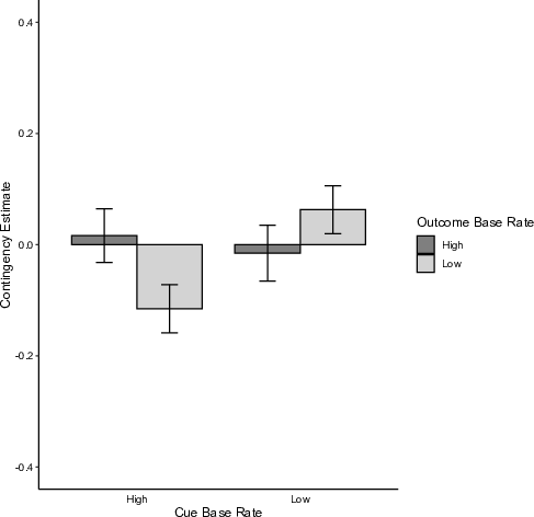
Figure 3: Results from Experiment 2. Estimates for contingency between cue (“yes”-answer by Politician X) and outcome (“yes”-answer by Politician Y) as a function of cue and outcome base rates. Error bars represent +/- 1 standard error.

---

Taken together, the findings from Experiment 2 substantiate our theorizing, showing that people are ready to infer different contingencies depending on the context. They also show that the alignment of base rates within contexts is a sufficient condition for base-rate-driven contingency illusions to occur.

4 General discussion

In the present paper we elaborated on contingency inferences from cue and outcome base rates. In two studies we found that people inferred conditional contingencies depending on the alignment of cue and outcome base rates. For contexts in which cue and outcome base rates were aligned (e.g., both high), perceived contingencies were more positive than for contexts in which cue and outcome base rates were misaligned (e.g., low cue base rate and high outcome base rate). These effects were observed although the actual contingencies within contexts were of the opposite sign. The pattern was consistent across different types of content regarding cue and outcome variables.

These findings contribute to the pseudocontingency framework (Fiedler et al., 2009; Fiedler et al., 2013) and demonstrate that people rely on univariate base rates to infer contingencies between binary predictor and outcome variables, which can result in biased contingency perception. However, they force a reconceptualization of pseudocontingencies, for they can no longer be seen as a uniform inference that relies on ecological correlations.

4.1 Aligned base rates vs. ecological correlations

As noted above, an ecological correlation refers to the correlation between cue and outcome base rates across ecologies (Robinson, 1950). Notably, the ecological correlation in previous trial-by-trial learning experiments always implied the same contingency as did the alignment of base rates (Fiedler & Freytag, 2004; Meiser & Hewstone, 2004; Vogel, Freytag, et al., 2013). That is, there were contexts in which cue and outcome base rates were both low and other contexts in which they were both high. Accordingly, outcome base rates increased with cue base rates (i.e., an ecological correlation). Throughout the present studies, we implemented a condition in which the observable ecological correlation was, in fact, zero. Nevertheless, we found systematic effects of the alignment of base rates within contexts. Thus, the present findings are the first to demonstrate clearly that the alignment of base rates within contexts can drive the pseudocontingency illusion independent of an ecological correlation.

4.2 Aligned base rates as source of judgmental biases

Obviously, the reliance on aligned base rates can lead to systematic biases. This was the case in the present experiments, where judgments diverged from actual contingencies. In fact, the demonstration of within-context contingency estimates is compatible with a large body of research on illusory correlations, usually studied in single contexts (e.g., Hamilton & Gifford, 1976)³. Notably, the distributions used in illusory correlation research share the same characteristics as the within-context distributions in the present studies. That is, one cue level is more frequent than the other, one outcome level is more frequent than the other, but the actual correlation between the frequent cue and the frequent outcome is zero or even negative. However, most prominent illusory correlation accounts propose that contingency illusions occur due to insufficient processing of joint occurrences (e.g., Hamilton & Gifford, 1976; Fiedler, 1991; Kutzner et al., 2011b; Smith, 1991). For instance, people may pay more attention to the double distinct event resulting from the combination of the numerical minor cue level and the numerical minor outcome level (Hamilton & Gifford, 1976). However, for a critical test of base-rate driven contingency inferences, we presented cue and outcome information on different occasions, so no joint observations were available (cf. Fiedler & Freytag, 2004).

Thus, in combination with previous research on pseudocontingencies (Fiedler et al., 2009), the present findings indicate that the reliance on aligned base rates serves as a parsimonious explanation that can account for illusory correlations in both a) standard illusory correlation paradigms in which participants have access to joint cue and outcome observations in a single context (Eder et al., 2011; Ernst et al., 2019; Hamilton & Gifford, 1976; for reviews, see, Costello & Watts, 2019; Mullen & Johnson, 1990), and b) more complex paradigms in which participants have access to joint cue and outcome observations from multiple contexts (e.g., Fiedler & Freytag, 2004; Meiser & Hewstone, 2004). Moreover, and different from illusory correlation accounts that rely on joint frequencies, it can accommodate findings obtained from c) single-context paradigms where participants do not have contingent observations but aggregated cue and outcome base rates (Vogel & Kutzner, 2017), and finally, d) findings from multi-context paradigms in which cue and outcome information is presented on different occasions (e.g., Exp. 2 in Fiedler & Freytag, 2004).

4.3 Aligned base rates as a smart heuristic

Though the reliance on aligned base rates is error-prone and can lead to illusory correlations, it does not necessarily fail but can enable sound decisions. Two arguments in favor of an alignment heuristic have been made so far. The first argument made in the literature (Kutzner et al., 2011a) is that population contingencies drive the alignment of base rates in observed samples. If the contingency in the population is perfectly positive, so that Δ p = 1.0, the base rates in a drawn sample are necessarily aligned, whereas a population contingency of Δ p = 0 allows base rates in a sample to be aligned or misaligned. The second argument rests on combinatory considerations and shows that the alignment of skewed base rates restricts the possible range of contingencies (Fiedler et al., 2013, Vogel & Kutzner, 2017). For example, if cue and outcome base rates are both high, e.g., p = .75, as was the case in the present studies, the minimum contingency is Δ p = −.33, that is the value realized in the present studies. However, the upper bound is not restricted and can reach the theoretical maximum of Δ p = +1.0. Thus, the alignment of base rates (or lack thereof) is indeed informative about the contingency, even more so when the skew is more extreme.

4.4 Aligned base rates: a comparison with prominent models

Whereas pseudocontingencies allow for contingency inferences from univariate base rates, most accounts – rule-based or associative (Allan, 1993) – are not directly suited to explain contingency judgments in the case of separated observations. Instead, they presume that people make contiguous cue-outcome observations, or at least that they hold some representation of joint cue-outcome observations (i.e., the cell entries of a 2×2 table; see Figure 1). Nevertheless, it appears worthwhile to test if the current results can be accommodated by such accounts for the following reasons: First, participants may be able to match observations from memory (e.g., they may be able to recollect the cue value for a given patient when they learn about the patient’s outcome). Second, pseudocontingencies may actually simulate pairwise cue-outcome observations. That is, people may use the aligned base rates to simulate possible joint observations (Vogel & Kutzner, 2017), which serve as a basis to apply rules or even to generate associations.

Therefore, we compared the observed contingency judgments with a formalization of PCs and three prominent accounts: the Δ p– and the Δ D rule as prominent examples of rule-based accounts (Allan, 1993; De Houwer & Beckers, 2002), and different instantiations of the Rescorla-Wagner model (Rescorla & Wagner, 1972) as one of the most prominent examples of associative learning theories. As for Δ p, we used the standard formulation by Jenkins & Ward (1965):

with a, b, c, and d, representing the joint frequencies of X+, X−, Y+, and Y−, respectively (see Table 1). Likewise, we used Δ D, also known as sum of diagonals, by calculating the difference between the compatible and the incompatible observations (Inhelder & Piaget, 1958; Shaklee & Tucker, 1980),

Next, to derive predictions from the Rescorla-Wagner Model, we ran a series of simulations using the Rescorla & Wagner Model Simulator Version 5 software (Chung et al., 2018). As for the associability parameters, α and β , we used the same values as Matute et al. (2019) who had demonstrated a cue-density effect, an outcome density-effect, as well as an interaction resulting from a strong incremental effect when cue and outcome density are both high (i.e., α and β ).

However, to best capture the experimental scenario, we specified models that yield associations of two mutually exclusive present cues, X vs. Y, with mutually exclusive present outcomes, positive versus negative. As an approximation of Δ p-scores, we then computed contingency indices by subtracting the relative associative strength for Cue Y, V_Y+ − V_Y−, from the relative associative strength for Cue X, V_X+ − V_X−. The first model is a model treating observations from different contexts as independent. This model yields cue-outcome associations for each of the within-context distributions. Thus, this model is comparable to a between-participants design in which a participant sees one of the four contexts. The second model simulates the association of cue and outcome when treating different contexts as four learning phases, thus a within-participants design with repeated measures of contingency judgments. To approximate the role of the context variable, the model was a compound cue model, with compounds of cue and context. Hence, this model yields indices of associative strength between cue and outcome per context (e.g., V_X+A as the association between Therapy X and desirable outcome for Disease A). This second model is sensitive to the order of contexts. We therefore modelled all orders that were implemented in the experiments as different counter-balancing conditions. However, for the sake of compatibility, we aggregated the predictions across orders just like we did in the analyses of the experimental data. Detailed results and input files of the simulation can be found in the online repository, https://osf.io/h57w3/?view_only=8578fb83e3644245a90219fe5561c5fc.

Lastly, the alignment rule reported in the introduction makes only qualitative predictions concerning the sign of the contingency. However, a rough quantification of a pseudocontingency alignment (PCA) rule can be derived from Kutzner (2009):

Although this formula was specified to describe the alignment of base rates, we use it as a proxy for contingency judgments (for ratios .1 < p(x)/p(y) < 10).

---

Table 2: Comparison of predictions and outcomes per context.

	Context
	A (HC,HO)	B (HC,LO)	C (LC,HO)	D (LC,LO)
Expected Judgment
Δ D-rule	.0	.0	.0	.0
Δ p-rule	−.33	+.33	+.33	−.33
RW (independent)	−.21	+.23	+.23	−.24
RW (compound cue)	−.19	+.03	+.01	−.20
PCA	+.23	−.23	−.23	+.23
Observed Judgment
Study1	+.12	−.24	−.02	+.18
Study2	+.02	−.12	−.02	+.06
Note. HC = High Cue Density, LC = Low Cue Density, HO = High Outcome Density, LO = Low Outcome Density, RW = Rescorla-Wagner Model, PCA = Pseudocontingency Alignment.

---

As can be derived from Table 2, the Δ D-rule predicts the same zero contingency in each and every context. The Δ p-rule, considered to be normative by several scholars (Jenkins & Ward, 1965, Allan, 1993), produces negative contingencies for contexts A and D, but positive contingencies for contexts B and C. The Rescorla-Wagner Model for independent observations produces the same qualitative pattern, though the contingencies are weaker. Qualitatively the same predictions are made when modelling compounds of cue and context. Finally, the pseudocontingency algorithm produces positive contingencies for contexts with aligned base rates, A and D, but negative contingencies for misaligned base rates, B and C.

Observed contingencies show the same pattern as the pseudocontingency algorithm. While the pseudocontingency algorithm can accommodate the qualitative pattern, it should be noted that the observed contingencies are weaker in size. One way to address the divergence is by merely adjusting the pseudocontingency algorithm using a calibration coefficient. As an alternative, one may conjecture that people use mixed algorithms. For instance, people may apply the normative Δ p rule for those instances they can recollect, but apply the alignment rule for instances when a reconstruction of paired observations is not possible (see Lachnit et al., 2008, for a discussion of the weighted impact of configural cues). The contingency judgment may therefore reflect a combination of strategies depending on their applicability to the data that can be recollected at the point of judgment. In fact, this notion is corroborated by previous research showing that pseudocontingencies do not only occur for subsequent cue-outcome presentations but also for simultaneous presentations. Yet, base rate effects are weaker for simultaneous presentations, and judgments are closer to the actual stimulus contingency (e.g., Exp. 2 in Fiedler & Freytag, 2004). Lastly, the small contingency estimates may also reflect participants’ uncertainty. The present paradigm forced participants to judge contingencies from small samples (i.e., 12 observations per context), thus regressive estimates may reflect that the sample contingency was considered unreliable (but see Kutzner et al., 2008 for pseudocontingencies from large samples).

Taken together, the simulation results show that pseudocontingencies do not mimic associative learning, at least with regard to the models under study, which assume contiguous presentation. This conclusion is of course preliminary, and novel extensions adapted to explain higher-order conditioning from subsequent observations might capture the process. In the present studies, a person may learn a connection between two conditioned stimuli, here the therapy and a given disease, and then learn a connection between that disease and the health condition. Hence, the resulting representation may link cue and outcome via the context. In other words, the present finding may not reflect a rule-based inference but actually follow from associative learning as conceived in prominent models applicable to sensory preconditioning (see Holyoak & Cheng, 2011).

4.5 Aligned base rates: informational requirement and applicability

As is evident from the present studies, people are indeed sensitive to the context. They are also able to learn base rates (see Fiedler et al., 2009) and thus meet the requirements for conditional contingency inferences from the alignment of base rates. However, it cannot be expected that people always learn and use the alignment of base rates as they did in our studies. In the last few paragraphs, we want to speculate when and why decision makers may (not) rely on aligned base rates.

One obvious advantage of the reliance on aligned base rates is that they allow for more differentiated judgments than the ecological correlation, that is, the inference of contingencies conditional on the context. However, this advantage counteracts the presumed advantage of pseudocontingencies over proper contingency assessment. As argued by Fiedler et al. (2009), pseudocontingencies may be used even in the presence of joint cue and outcome observations because the representation of joint cue and outcome frequencies is overwhelming while the univariate base rates can be represented parsimoniously. Obviously, this argument only holds for a small number of contexts because context-wise pseudocontingencies require that decision makers learn each and every pair of aligned base rates. With an increasing number of contexts, the representation becomes more and more demanding. Thus, in case of four contexts (as in the present experiments), people may make context-dependent inferences. However, in cases with more than four contexts, a context-wise representation of base rates appears implausible (Miller, 1956), and people may shift to an unconditional contingency inference.

The ecological correlation, on the contrary, can be learned with less effort. Though the mathematically correct calculation also requires that people know all the pairwise base rates, the ecological correlation can be represented as a single piece of information that is updated for each incoming information. Notably, it is not only possible to represent the ecological correlation in a parsimonious fashion. The ecological correlation also has some distinct areas of applicability, such as correlation inferences about present-absent distinctions (see Footnote 1) or continuous variables. Take, for example, a continuous predictor and criterion, both normally distributed. Learning that the mean of the predictor correlates with the mean of the criterion across contexts, allows to infer a correlation between the two, without any assumption about skewed base rates. This is not to rule out that the alignment rule is also applicable to continuous variables. Perhaps people infer a positive correlation between two variables that are skewed in the same direction (also see Fiedler & Freytag, 2004). However, learning the skew of a distribution is more demanding than learning the base rates from binary variables. Moreover, the rational arguments for relying on aligned base rates that apply to binary variables do not apply for continuous variables (Vogel & Kutzner, 2017). That is, different from binary variables, the joint skew of continuous variables does not restrict the range of possible correlations.

Finally, contingency detection is not usually a task pursued for its own sake, but a prerequisite for understanding the world (Crocker, 1981). Thus, the reliance on base rates – via the alignment or the ecological correlation – versus actual contingencies – conditional or unconditional – is a question of affordances. Acting as an intuitive statistician (Peterson & Beach, 1967), the decision maker is faced with a multi-level problem and needs to decide which level to focus on and which question to answer. For example, a decision maker might wonder whether, at the country level, good health conditions depend on high vaccination rates? At the individual level, does a person’s health status depend on Vaccine X? And does it depend on Vaccine X among people suffering from a certain virus variant? To address these questions, decision makers do not rely on data alone, but try to integrate them into their prior expectations about causal relations (Matute et al., 2019; Waldmann, 1996). Specifically, tri-variate relations can imply different causal structures – suppression, mediation, confound, or moderation. In this vein, research on contingency detection in Simpson’s Paradox showed that decision makers are quite sensitive to the specific question at hand. Depending on their hypotheses and causal assumptions, they rely on unconditional or conditional contingencies (Schaller, 1994; Schaller et al., 1996; Spellman, 1996; Spellman et al., 2001). Thus, future research could vary the (implicit) underlying causal structure and assess its consequences for the reliance on alignment of base rates, ecological correlation, or on individuating contingency information in contingency detection. Moreover, future research may profit from changes in the presentation mode. In order to study the mechanism underlying contingency inferences in the absence of joint cue-outcome observations, we used a presentation blocked by cue and outcome. However, memory constraints cause that people sometimes rely on base rates though contingent observations are available (Eder et al., 2011). From an adaptive cognition perspective, one would expect people to choose the most parsimonious strategy to test plausible mechanisms (main effect or moderations; Novick & Cheng, 2004) in a selection process that also depends on information availability. Presented with joint cue-outcome observations, people may learn the actual contingency (Allan, 1993), but disregard base rate information altogether (Vogel et al., 2014).

After all, there is no single true covariation. Adaptive covariation assessment therefore depends on the question at hand (Pearl, 2014) – and also on which data is available. Starting with Robinson’s ecological correlations, researchers have found different ways to model covariation from aggregate data (King, 2013), and future research may reveal that this holds true for laypeople, too.

5 Conclusion

The present findings challenge the notion of a single theoretical explanation of pseudocontingencies based on ecological correlations (Fiedler & Freytag, 2004; Fiedler et al., 2007; Vogel et al., 2013). This account predicts that individuals use base rates to infer just one contingency (thus, the same contingency in every context) which follows the sign of the ecological correlation. However, the present research shows that individuals are able and willing to infer conditional contingencies from base rates within each and every context. Just as the ecological correlation, the alignment of base rates is not sufficient to inform contingency judgments. However, in absence of pairwise cue-outcome observations, the reliance on aligned base rates is a promising strategy that allows for context-wise contingency inferences.

References

*

Darmstadt University of Applied Sciences, Haardtring 100, 64295 Darmstadt/Germany; https://orcid.org/0000-0002-5768-1391. Email: tobias.vogel@h-da.de.

#

University of Mannheim. https://orcid.org/0000-0002-2124-0754.

$

Heidelberg University. https://orcid.org/0000-0001-5309-6008.

The authors thank Franziska Bott, Sophie Giel, and Thorsten Meiser for valuable comments.

Data are available at https://osf.io/h8qpg/.

Copyright: © 2022. The authors license this article under the terms of the Creative Commons Attribution 3.0 License.

1

Rooted in the literature on causal learning, many studies investigate contingency detection for present-absent distinctions. In such studies, judgments tend to converge with Δ p, but absent-absent observations have minor impact (i.e., cell-D insensitivity, see Arkes & Harkness, 1983; Hattori & Oaksford, 2007; Mata, Garcia-Marques, Ferreira & Mendonça, 2015). Note that in our example and the remainder of the paper, binary events are dimensional (e.g., X vs. Y), so there are no absent trials. Instead, absence of one cue, X, entails the presence of the other, Y. By definition, we refer to a positive contingency as an association between the levels of cue and outcome that appear first in the 2×2 table (upper row for the cue; left column for the outcome). Thus, if the contingency describes the association between “Therapy X” and “improved health”, “Therapy X” is the cue, and “improved health” is the outcome. In turn, high cue base rate refers to p(Therapy X) > .5, whereas low cue base rate refers to p(Therapy X) < .5, etc.

2

Schaller and O’Brien (1992) presented participants with a Simpson’s Paradox (1951). In such a tri-variate distribution the average conditional contingency (i.e., the partial contingency) between cue and outcome differs from their unconditional (i.e. pooled) contingency. They found that participants disregarded the context variable and based their contingency judgments on the unconditional contingency. For a rational analysis of Simpson’s Paradox, see Pearl (2014).

3

As mentioned in the introduction, pseudocontingencies in single contexts have been conceived of as implicit ecological correlations. That is, starting with an ignorant prior of p_cue = p_outcome = .5, aligned base rates imply a positive ecological correlation whereas misaligned base rates imply a negative ecological correlation (Fiedler et al., 2007; Vogel, Kutzner, et al., 2013). However, in light of the present findings, one would need to assume that individuals do not learn the ecological correlation, but infer four independent implicit ecological correlations. After all, an explanation of the present findings in terms of implicit ecological correlations within contexts is not plausible, and in any case less parsimonious than the proposed explanation.

This document was translated from L^AT_EX by H^EV^EA.

References

Allan, L. G. (1993). Human contingency judgments: Rule based or
associative? Psychological Bulletin, 114(3), 435–448.
https://doi.org/10.1037/0033-2909.114.3.435.
Arkes, H. R., & Harkness, A. R. (1983). Estimates of contingency between
two dichotomous variables. Journal of Experimental Psychology:
General, 112(1), 117.
https://doi.org/10.1037/0096-3445.112.1.117.
Blanco, F., Matute, H., & Vadillo, M. A. (2013). Interactive effects of
the probability of the cue and the probability of the outcome on the
overestimation of null contingency. Learning & Behavior,
41(4), 333–340. https://doi.org/10.3758/s13420-013-0108-8.
Bott, F. M., & Meiser, T. (2020). Pseudocontingency inference and choice:
The role of information sampling. Journal of Experimental
Psychology: Learning, Memory, and Cognition, 46(9), 1624–1644.
https://doi.org/10.1037/xlm0000840.
Chung, B., Mondragón, E., & Alonso, E. (2018). Rescorla & Wagner
Simulator+ © Ver. 5.[Computer software]. St. Albans, UK: CAL-R. Available
from https://www.cal-r.org/index.php?id=R-Wsim-plus.
Costello, F., & Watts, P. (2019). The rationality of illusory correlation.
Psychological Review, 126(3), 437–450.
https://doi.org/10.1037/rev0000130.
Crocker, J. (1981). Judgment of covariation by social perceivers.
Psychological Bulletin, 90(2), 272–292.
https://doi.org/10.1037/0033-2909.90.2.272.
De Houwer, J., & Beckers, T. (2002). A review of recent developments in
research and theories on human contingency learning. The Quarterly
Journal of Experimental Psychology B: Comparative and Physiological
Psychology, 55B(4), 289–310.
https://doi.org/10.1080/02724990244000034.
Eder, A. B., Fiedler, K., & Hamm-Eder, S. (2011). Illusory correlations
revisited: The role of pseudocontingencies and working-memory capacity.
The Quarterly Journal of Experimental Psychology,
64(3), 517–532. https://doi.org/10.1080/17470218.2010.509917.
Ernst, H. M., Kuhlmann, B. G., & Vogel, T. (2019). The origin of illusory
correlations: Biased judgments converge with inferences, not with biased
memory. Experimental Psychology, 66(3), 195–206.
https://doi.org/10.1027/1618-3169/a000444.
Faul, F., Erdfelder, E., Lang, A.-G., & Buchner, A. (2007). G*Power 3: A
flexible statistical power analysis program for the social, behavioral,
and biomedical sciences. Behavior Research Methods,
39(2), 175–191. https://doi.org/10.3758/BF03193146.
Fiedler, K. (1991). The tricky nature of skewed frequency tables: An
information loss account of distinctiveness-based illusory correlations.
Journal of Personality and Social Psychology, 60(1),
24–36. https://doi.org/10.1037/0022-3514.60.1.24.
Fiedler, K. (2010). Pseudocontingencies can override genuine contingencies
between multiple cues. Psychonomic Bulletin & Review,
17(4), 504–509. https://doi.org/10.3758/PBR.17.4.504.
Fiedler, K., & Freytag, P. (2004). Pseudocontingencies. Journal of
Personality and Social Psychology, 87(4), 453–467.
https://doi.org/10.1037/0022-3514.87.4.453.
Fiedler, K., Freytag, P., & Meiser, T. (2009). Pseudocontingencies: An
integrative account of an intriguing cognitive illusion.
Psychological Review, 116(1), 187–206.
https://doi.org/10.1037/a0014480.
Fiedler, K., Freytag, P., & Unkelbach, C. (2007). Pseudocontingencies in a
simulated classroom. Journal of Personality and Social
Psychology, 92(4), 665–677.
https://doi.org/10.1037/0022-3514.92.4.665.
Fiedler, K., Kutzner, F., & Vogel, T. (2013). Pseudocontingencies:
Logically unwarranted but smart inferences. Current Directions In
Psychological Science, 22(4), 324–329.
https://doi.org/10.1177/0963721413480171.
Fleig, H., Meiser, T., Ettlin, F., & Rummel, J. (2017). Statistical
numeracy as a moderator of (pseudo)contingency effects on decision
behavior. Acta Psychologica, 174, 68-79.
https://doi.org/10.1016/j.actpsy.2017.01.002.
Hamilton, D. L., & Gifford, R. K. (1976). Illusory correlation in
interpersonal perception: A cognitive basis of stereotypic judgments.
Journal of Experimental Social Psychology, 12(4),
392–407. https://doi.org/10.1016/S0022-1031(76)80006-6.
Hattori, M., & Oaksford, M. (2007). Adaptive non-interventional
heuristics for covariation detection in causal induction: Model comparison
and rational analysis. Cognitive Science, 31(5),
765–814. https://doi.org/10.1080/03640210701530755.
Holyoak, K. J., & Cheng, P. W. (2010). Causal learning and inference as a
rational process: The new synthesis. Annual Review of Psychology,
62(1), 135–163.
https://doi.org/10.1146/annurev.psych.121208.131634.
Jenkins, H. M., & Ward, W. C. (1965). Judgment of contingency between
responses and outcomes. Psychological Monographs: General And
Applied, 79(1), 1–17. https://doi.org/10.1037/h0093874.
King, G. (2013). A solution to the ecological inference problem.
Princeton University Press. https://doi.org/10.1515/9781400849208.
Kutzner, F. (2009). Pseudocontingencies–rule based and associative
(Doctoral dissertation).
Kutzner, F., Freytag, P., Vogel, T., & Fiedler, K. (2008). Base-rate
neglect as a function of base rates in probabilistic contingency learning.
Journal of the Experimental Analysis of Behavior, 90(1),
23–32. https://doi.org/10.1901/jeab.2008.90-23.
Kutzner, F., Vogel, T., Freytag, P., & Fiedler, K. (2011a). Contingency
inferences driven by base rates: Valid by sampling. Judgment and
Decision Making, 6(3), 211–221.
Kutzner, F., Vogel, T., Freytag, P., & Fiedler, K. (2011b). A robust
classic: Illusory correlations are maintained under extended operant
learning. Experimental Psychology, 58(6), 443–453.
https://doi.org/10.1027/1618-3169/a000112.
Inhelder, B., & Piaget, J.P. (1958). The growth of logical
thinking from childhood to adolescence: An essay on the construction of
formal operational structures. Routledge.
Lachnit, H., Schultheis, H., König, S., Üngör, M., & Melchers, K. (2008).
Comparing elemental and configural associative theories in human causal
learning: A case for attention. Journal of Experimental
Psychology: Animal Behavior Processes, 34(2),
303–313. https://doi.org/10.1037/0097-7403.34.2.303.
Lee, M. D., & Wagenmakers, E.-J. (2013). Bayesian cognitive
modeling: A practical course. Cambridge University Press.
Leiner, D. J. (2014). SoSci Survey (Version 2.5.00-i) [Computer software].
Available at http://www.soscisurvey.com.
Mata, A. (2016). Judgment of covariation: A review. Psicologia,
30(1), 61–74. https://doi.org/10.17575/rpsicol.v30i1.1082.
Mata, A., Garcia-Marques, L., Ferreira, M. B., & Mendonça, C. (2015).
Goal-driven reasoning overcomes cell D neglect in contingency judgements.
Journal of Cognitive Psychology, 27(2), 238–249.
https://doi.org/10.1080/20445911.2014.982129.
Matute, H., Blanco, F., & Díaz-Lago, M. (2019). Learning mechanisms
underlying accurate and biased contingency judgments. Journal of
Experimental Psychology: Animal Learning and Cognition, 45(4),
373–389. https://doi.org/10.1037/xan0000222.
Meiser, T., & Hewstone, M. (2004). Cognitive processes in stereotype
formation: The role of correct contingency learning for biased group
judgments. Journal of Personality and Social Psychology,
87(5), 599–614. https://doi.org/10.1037/0022-3514.87.5.599.
Meiser, T., Rummel, J., & Fleig, H. (2018). Pseudocontingencies and choice
behavior in probabilistic environments with context-dependent outcomes.
Journal of Experimental Psychology: Learning, Memory, and
Cognition, 44(1), 50–67. https://doi.org/ 10.1037/xlm0000432.
Miller, G. A. (1956). The magical number seven, plus or minus two: Some
limits on our capacity for processing information. Psychological
Review, 63(2), 81. https://doi.org/10.1037/h0043158.
Morey, R. D., & Rouder, J. N. (2018). BayesFactor: Computation of
Bayes Factors for common designs.
https://cran.r-project.org/package=BayesFactor.
Mullen, B., & Johnson, C. (1990). Distinctiveness-based illusory
correlations and stereotyping: A meta-analytic integration.
British Journal of Social Psychology, 29(1), 11–27.
https://doi.org/10.1111/j.2044-8309.1990.tb00883.x.
Novick, L. R., & Cheng, P. W. (2004). Assessing interactive causal
influence. Psychological Review, 111(2), 455–485.
https://doi.org/10.1037/0033-295X.111.2.455.
Pearl, J. (2014). Comment: Understanding Simpson’s Paradox. The
American Statistician, 68(1), 8–13,
https://doi.org/10.1080/00031305.2014.876829.
Peterson, C. R., & Beach, L. R. (1967). Man as an intuitive statistician.
Psychological Bulletin, 68(1), 29–46.
https://doi.org/10.1037/h0024722.
Rescorla, R. A., & Wagner, A. R. (1972). A theory of Pavlovian
conditioning: Variations in the effectiveness of reinforcement and
non-reinforcement. In A. H. Black & W. F. Prokasy (Eds.),
Classical conditioning II: Current research and theory (pp.
64–99). Appleton-Century-Crofts.
Robinson, W. S. (1950). Ecological correlations and the behavior of
individuals. American Sociological Review, 15(3), 351–357.
Reprint at https://doi.org/10.1093/ije/dyn357.
Schaller, M. (1994). The role of statistical reasoning in the formation,
preservation and prevention of group stereotypes. British Journal
of Social Psychology, 33(1), 47–61. https://doi.org/10.1111/j.2044-8309.1994.tb01010.x.
Schaller, M., Asp, C. H., Roseil, M. C., & Heim, S. J. (1996). Training in
statistical reasoning inhibits the formation of erroneous group
stereotypes. Personality and Social Psychology Bulletin,
22(8), 829–844. https://doi.org/10.1177/0146167296228006.
Schaller, M., & O’Brien, M. (1992). “Intuitive analysis of covariance” and
group stereotype formation. Personality and Social Psychology
Bulletin, 18(6), 776–785.
https://doi.org/10.1177/0146167292186014.
Shaklee, H., Tucker, D. (1980) A rule analysis of judgments of covariation
between events. Memory & Cognition, 8, 459–467.
https://doi.org/10.3758/BF03211142.
Simpson, E. (1951). The interpretation of interaction in contingency
tables. Journal of the Royal Statistical Society. Series B
(Methodological), 13(2), 238–241. https://www.jstor.org/stable/2984065.
Singmann, H., Bolker, B., Westfall, J., Aust, F., & Ben-Shachar, M. S.
(2020). afex: Analysis of Factorial Experiments.
https://cran.r-project.org/package=afex.
Smith, E. R. (1991). Illusory correlation in a simulated exemplar-based
memory. Journal of Experimental Social Psychology,
27(2), 107–123. https://doi.org/10.1016/0022-1031(91)90017-Z.
Spellman, B. A. (1996). Acting as intuitive scientists: Contingency
judgments are made while controlling for alternative potential causes.
Psychological Science, 7(6), 337–342.
https://doi.org/10.1111/j.1467-9280.1996.tb00385.x.
Spellman, B. A., Price, C. M., & Logan, J. M. (2001). How two causes are
different from one: The use of (un)conditional information in
Simpson’s paradox. Memory & Cognition,
29(2), 193–208. https://doi.org/10.3758/BF03194913.
Vogel, T., Freytag, P., Kutzner, F., & Fiedler, K. (2013).
Pseudocontingencies derived from categorically organized memory
representations. Memory & Cognition, 41(8), 1185–1199.
https://doi.org/10.3758/s13421-013-0331-8.
Vogel, T., & Kutzner, F. (2017). Pseudocontingencies in consumer choice:
Preference for prevalent product categories decreases with decreasing set
quality. Journal of Behavioral Decision Making, 30(5),
1193–1205. https://doi.org/10.1002/bdm.2034.
Vogel, T., Kutzner, F., Fiedler, K., & Freytag, P. (2013). How majority
members become associated with rare attributes: Ecological correlations in
stereotype formation. Social Cognition, 31(4), 427–442.
https://doi.org/10.1521/soco\_2012\_1002.
Vogel, T., Kutzner, F., Freytag, P., & Fiedler, K. (2014). Inferring
correlations: From exemplars to categories. Psychonomic Bulletin
& Review, 21(5), 1316–1322.
https://doi.org/10.3758/s13423-014-0586-5.
Waldmann, M. R. (1996). Knowledge-based causal induction. In D. R. Shanks,
K. Holyoak, & D. L. Medin (Eds.), Causal learning. (pp. 47–88).
Academic Press. https://doi.org/10.1016/S0079-7421(08)60558-7.
This document was translated from LATEX by