Judgment and Decision Making, Vol. 17, No. 4, July 2022, pp. 883-936
Stress and risk — Preferences versus noiseElle Parslow* Julia Rose# $ |
Abstract:We analyze the impact of acute stress on risky choice in a pre-registered laboratory experiment with 194 participants. We test the causal impact of stress on the stability of risk preferences by separating noise in decision-making from an actual shift in preferences. We find no significant differences in risk attitudes across conditions on the aggregate, using both descriptive analyses as well as structural estimations for risk aversion and different noise structures. Additionally, in line with the previous literature, we find statistically significant evidence for lower cognitive abilities being correlated with more noise in decision-making in general. We do not find a significant interaction effect between cognitive abilities and stress on noise levels.
Keywords: risk preferences, risk aversion, stress, laboratory stressor, Trier social stress test, cortisol
People make countless decisions each day, often involving uncertain outcomes. In addition, these decisions are often made in stressful situations, and it seems plausible that experienced stress will affect the type and quality of those choices. A classic high-stakes example where stress is likely to matter is trading on the stock market, but it is likely to matter in more mundane situations as well.
In this paper, we show that stress does not have a significant impact on risk preferences when controlling for errors in decision-making. Using a between-subject design with 194 subjects, we manipulate stress levels by inducing psychological stress with the Trier Social Stress Test for groups (TSST-G von Dawans et al., 2011). We measure risk attitudes with a series of risky choices in a Multiple Price List (MPL) method based on the methodology of (Andersson et al., 2016). The main contribution of our paper is that we are able to establish a causal relationship of the impact of stress on risk taking by accounting for noise. We use a particularly simple risk elicitation method to mitigate the potential errors in decision-making in the first place.1 In addition, we account for decision errors both in our descriptive analyses as well as parameter estimations, where the latter can additionally account for not only how frequently errors occur, but also in which particular decision within a choice list they happen. While our basic assumption is that people make choices that reflect their true preferences (i.e., choices are not completely random), we acknowledge that for some instances, observed choices can be mistakes. Identifying the particular point within a MPL where the error happens is important since we distinguish the two most common types of errors, Fechner errors, popularized by (HeyOrme, 1994) (where errors happen around the true switching point in a given MPL), and trembling hand errors (Luce, 1959) (which assigns some probability that a given choice is random).
As a further contribution, we have a larger sample than almost any related study, and consequently a higher power to detect potential effects: with our sample size of 194 participants, we have 90% power to find a Cohen’s d effect size of 0.47 (which represents a medium effect) with p = 0.05, and 90% power to find a Cohen’s d of 0.6 with p = 0.005. Our study design, hypotheses, and analyses are preregistered on OSF (Open Science Framework; link to the pre-analysis plan: https://osf.io/zgt7w/).
The findings of existing studies analyzing the impact of stress on risk preferences are mixed, and we identify errors in decision-making as a potential candidate that contributes to the lack in consensus. Studies report findings that range from increased risk aversion to increased risk seeking, and also include findings that do not report any treatment effect at all. In general, stress could affect risky choices in two ways. First, it could make people more risk seeking (or risk averse), and second, it could also increase decision errors. Decision errors can bias the measure of risk preferences even if the errors are random (HeyOrme, 1994,HarlessCamerer, 1994,Dave et al., 2010). If stress leads to increased decision errors compared to a baseline without stress, these errors have to be taken into account to make causal inferences on the impact of stress on risk preferences.
So far, the consequences of decision errors on the interpretation of elicited risk attitudes have not been taken into account. A variety of studies using different methods to elicit risk preferences are closely related to our study (see Table 1 in section 2), where only 2 out of 16 acknowledge the potential confounding effects of decision errors.
Accounting for decision errors is important. Without controlling for such noise, there is no clear causal interpretation of the impact of stress on measured risk attitudes, even more so in small samples. As pointed out above, decision errors can already bias the baseline measure, which has also gained attention in more recent studies (see Charness et al., 2013,HolzmeisterStefan, 2021, for example). Introducing stress and comparing elicited risk attitudes across treatments is further complicated by the fact that stress can have a detrimental effect on various cognitive processes (see Qin et al., 2009,McEwenSapolsky, 1995,Shields et al., 2016, for example). Cognitive abilities, in turn, have been shown to be inversely related to the propensity for displaying noise in decisions under risk (see Andersson et al., 2016,Andersson et al., 2020,Amador-Hidalgo et al., 2021, for example). In small samples with low power — as is the case for the vast majority of related studies (see Table 1 in section 2, where N denotes the number of subjects in the particular study) — those described effects complicate it even more to make causal claims about the impact of stress on risk preferences.
The definition of noise, or decision errors, in our setting is based on violations of monotonicity. In our experiment, subjects have to make a series of choices in a Multiple Price List (MPL) design based on (Andersen et al., 2006). Within a given price list, the decision maker has to chose between two lotteries, “left” and “right”. Both lotteries are depicted as a fair coin toss, and the outcomes of lottery “left” (depicted as “heads” and “tails”) are fixed for all decisions, as well as the “heads” option of lottery “right”. The only value that changes across decisions within the price list is thus outcome “tails” of lottery “right”. This outcome is increasing in value across decisions, making lottery “right” subsequently more attractive. As a consequence, a decision maker satisfying monotone preferences starting from choosing lottery “left” should switch only once to the right — in particular, not switch back to the less attractive option. A switch back to the less attractive option is considered as noise, and based on the argument of monotonicity only, without relying on further restrictive assumptions on the shape of the utility function. Please note that, in general, we do not make a qualitative statement of whether riskier choices are “better” or “worse” for a subject, our aim is to determine whether we observe a true shift in preferences in any direction. This is important, since taking risky decisions in general might be disadvantageous in some contexts but advantageous in other contexts.
Heterogeneity in noise across decision makers can induce a bias in the measurement of risk preferences, which is particularly important in a framework where such noise is expected to affect one treatment more than the other (StarckeBrand, 2016). Since accounting for such noise across treatments is the major contribution of our study, we illustrate its implications on the measurement of risk preferences based on the example by (Andersson et al., 2016), (Andersson et al., 2020). Imagine two experimental subjects, A and B, with the same underlying preferences. The difference between A and B is that A makes all decisions error-free, and B make a mistake with probability p > 0 at every single decision within a list. These errors can lead to a choice pattern where B switches back to the safer option after having chosen the risky option once, violating monotonicity (“reverse switches”). A common way to measure risk preferences is to count the number of safer choices, which immediately highlights the problem when noise is not accounted for: whereas A and B have the same underlying preferences, B appears to be more risk averse due to the reverse switches. If stress increases noise, accounting for this noise is important for a causal interpretation of treatment differences.
Excluding subjects with noise in decision-making in the analysis does not alleviate the problem, since it potentially removes an important source of variation. It is very likely that noise-prone subjects have different characteristics overall, such as lower cognitive abilities (c.f. Andersson et al., 2016,Andersson et al., 2020,Amador-Hidalgo et al., 2021, for example), and potentially also different (baseline) risk attitudes after controlling for noise.
To account for noise in our analyses, we present both descriptive analyses and structural estimations of risk aversion and noise parameters, where the latter accounts for both the extent and location of noise within the choice lists. While presenting descriptive statistics about the frequency of observed reverse switches as a measure of decision errors gives an important first insight, such an analysis cannot distinguish between the type of errors that can occur. For such a distinction, not only the frequency, but the exact location of the reverse switches within a choice list is important. In our analyses, we consider two common types of errors: The first type is a random error that occurs some probability at every choice, as in the example above. This can be illustrated in our task as an error that occurs by a simple mistake when wanting to select the preferred option but by mistake clicking on the less preferred option, and is called a trembling hand error, put forward by (Luce, 1959). The second type is the so called Fechner error, popularized by (HeyOrme, 1994), where reverse switches occur before and after (i.e., close to) the actual switching point. This type of error happens when subjects evaluate the two lotteries in terms of (subjective) expected outcomes, and make mistakes in calculating those outcomes. The distinction between error structures by using structural estimation techniques is an important information – we can analyze whether stress not only changes the frequency of observed errors, but also whether the type of errors changes.
Taken together, and given the somewhat unclear findings for the direction of the effect that acute stress has on risk preferences, we derive the following three pre-registered hypotheses. In particular, we expect that risk-seeking increases under stress, based on the majority of the related literature pointing in a similar direction as outlined in Table 1 in the literature review in section 2:
At the aggregate level, we find no evidence that stress affects risk attitudes. These findings hide some potentially interesting heterogeneous effects across sub-populations, which we address with exploratory analyses. All analyses addressing different hypotheses than pre-registered are included in a separate section and clearly labeled as exploratory analyses. The results suggest that female participants seem to make slightly more risk averse choices when under stress compared to the no stress condition. We can show that this is not driven by more noisy choices, but might be a true shift in their risk attitudes. For male participants, we do not observe a difference in the level of risk aversion across conditions.
In the full sample, cognitive abilities are negatively correlated with the level of noise in decisions, and this holds independent of whether participants are in the stress condition or not. In particular, the interaction between treatment and cognitive abilities is not significant, showing that stress does not disproportionately increase noise for subjects with lower cognitive abilities in our task design.
Given that the results are not significant in our frequentist analyses, we add Bayesian analyses to present a more comprehensive picture of our data. These analyses are not pre-registered, but are an important addition to interpret our findings beyond a non-conclusive statement reporting the insignificant results. The Bayesian analyses are included in the main analysis as supportive information. The results reveal that there is indeed substantial evidence in favor of no changes in risk taking under acute stress, and that the evidence on gender differences in the impact of stress on risk attitudes is inconclusive. Bayesian linear regressions additionally support the findings that there is an inverse relation between cognitive abilities and noise.
The rest of the paper is organized as follows. Section 2 provides a brief overview of the most closely related literature, pointing out the differences to our study. This is followed by a detailed description of our experimental design and the procedures involved in the induction and measurement of the stress response in section 3. Section 4 presents descriptive results as well as parameter estimations, including exploratory analyses which we did not pre-register in the separate subsection 4.5. Section 5 discusses the limitations of our work.
The impact of stress on risky decision-making has been investigated in several experimental studies with different methodologies for the induction of stress as well as the elicitation of risk attitudes. However, even among the studies using a similar methodology, there is no clear consensus on whether or how stress shifts risk preferences. In particular, there is very little to no discussion about the potential impact of stress on noise in decision-making and the potential problems associated with such effects in the causal interpretation of treatment differences.
To put the methods and literature outlined in the following into perspective to our present study, we briefly describe the most important basic information of our design: We use a psychological stress induction for groups (TSST-G; von Dawans et al., 2011), with a 35 minute delay between the start of the stress induction and the risk task. This task combines high levels of social-evaluative threat and uncontrollability in a group format with several phases, including a public speaking task in the form of a mock job interview, and a mental arithmetic task with serial subtractions. The main feature of the TSST-G is that it triggers both physical and psychological stress responses, and therefore also induces the subjective feeling of being stressed. This feature is also the main difference to the other methods used in the literature as outlined in more detail below, where mainly psychological stress responses are triggered. To check for a successful treatment manipulation, we take saliva samples to measure changes in cortisol levels as well as a self-reported negative affect scale (part of the PANAS scale; Watson et al., 1988).
For eliciting risk attitudes, we use a simple multiple price list format (Andersson et al., 2016), where choices are binary (between a “left” and “right” lottery), where each lottery is depicted by a simple coin toss. An important feature of our risk elicitation task is that we do not have varying probabilities across decisions, which makes it simple to understand for subjects, but also does not introduce potential other effects, such as non-linear probability weighting (see, e.g., Quiggin, 1982). Additionally, our outcomes are fixed for the “safe” option (which is always presented on the left part of the screen) and only vary in one outcome dimension in the “risky” option (which is always presented on the right part of the screen). A more detailed description of the task design is given in section 3.2. These are also the main differences to the other designs as used in the related literature, which involve more complicated elicitation methods (such as the method by (HoltLaury, 2002) where probabilities vary, for example), or more gamified measures of risk (such as the Game of Dice Task by (Brand et al., 2005) or the Balloon Analogue Risk Task by (Lejuez et al., 2002), both as outlined in detail below).
Results in related papers range from less risk seeking under stress to increased risk seeking under stress, also including no significant effect at all. To provide an orientation for the related findings using a similar methodology to ours, Table 1 summarizes the respective results together with the key features of the experimental implementation. In addition, we outline in how far the studies account for, or at least discuss, the implications of noise in decision-making under stress.
Table 1: Previous studies of effects of stress on risky choice - similar methodology. The first part of the table presents an overview of the studies most closely related to ours (same stressor and similar risk elicitation task). The second part of the table presents studies that are closely related with respect to the stressor, but use a different risk elicitation methodology. The third part of the table presents studies using a similar risk elicitation task, but a different stressor.
N Effect on risk taking/aversion Accounting for noise (under stress) [1] 67 No significant effect. (all male sample) — [2] 75 Increased RT for cortisol responders (gain domain only). — [3] 26 Increased RA for gains, no effect loss domain. — [4] 146 Increased RA for male cortisol responders only, no effect for women. Exclude multiple switches in the main text, robustness check in online appendix – no check whether there are differential effects on noise between treatments. [5] 352 Increased RT (directly after stress only). — [6] 75 Increased RT. — [7] 34 Increased RT for high social anxiety group, no effect low group. — [8] 85 No significant effect. — [9] 40 Increased RA 5 min and 18 min after stress relative to CC, increased RT 28 min after stress — [10] 80 Increased RA in loss domain, no effect gain domain. — [11] 33 No significant effect. — [12] 126 Increased RT under stress for GDT as only task. — [13] 208 Increased willingness to speculate for men, decreased willingness to speculate for women. — [14] 69 Increased RT for gambles with low risk, increased RA for gambles with high risk — [15] 120 No significant effect. Within-subject design where the identical decision-making task is repeated one day apart. They have a measure for consistency of choices across both conditions as a separate variable. No actual control for consistency when testing for differences in risk attitudes. [16] 143 No significant effect. — All described effects are relative to the control condition (no-stress condition). RA: risk aversion. RT: risk taking. MPL: multiple price list. GDT: Game of Dice Task. BART: Balloon Analogue Risk Task. TSST(-G): Trier Social Stress Test (for Groups). (SE-)CPT: (Socially Evaluated-)Cold Pressor Test.. SET: Speculation Elicitation Task.
In general, predicting the direction of the effect of stress on risk preferences (for example, in increasing or decreasing risk seeking) is complicated by several factors. As suggested by a recent meta-analysis by (StarckeBrand, 2016), the effect of acute stress on decision-making might partly depend on the timing of the stressor and stress hormone release relative to the decision task, even though the authors do not find statistically significant evidence for that. Additionally, they suggest individual and demographic variables such as gender or age as potential moderator variables, but again, fail to find statistically significant results. A number of studies includes several different directional results, depending, for example, on the domain of risk taking (gains or losses) or explanatory variables (e.g., testing gender differences).
The predictability of an effect of stress on risk taking is also complicated by the great diversity of induction methods. Stress induction targets physical or psychological stress, where the latter can be actual or anticipated. To measure a successful treatment manipulation, to most common indicator for a successful stress induction in experimental studies is the salivary cortisol level. Cortisol is one of the glucocorticoids that are released during activation of the hypothalamic–pituitary–adrenal (HPA) axis, which has been shown to have possible impacts and consequences for decision-making (van den Bos et al., 2009).
Table 1 gives an overview of the studies that are most closely related to our experimental design, either using both the TSST(-G) and a lottery task, or either of the two in combination with a different method. Studies [1] to [5] use very similar methods to ours, combining the TSST(-G) and a lottery task. Lottery choice tasks mainly involve some form of asking participants to choose between a safe(r) (gamble) payment and a (riskier) gamble, where probabilities and payoffs are given explicitly (see, e.g., HoltLaury, 2002). In contrast to our design, probabilities and several outcomes vary across conditions, making it more involved for participants to calculate expected outcomes and evaluate the given options.
Studies [6] to [13] use the TSST similar to us, but use different methods to elicit risk attitudes: the Balloon Analogue Risk Task (BART, Lejuez et al., 2002), the Game of Dice Task (GDT, Brand et al., 2005), and a speculation elicitation task (SET, Janssen et al., 2019,MoinasPouget, 2013). The BART is a gamified version of a risk elicitation task, which involves pumping air into a balloon on screen until the subject either decides to stop or the balloon explodes. Each round a new balloon appears on screen, and balloons have different probabilities of exploding per pump of air across rounds. The GDT involves a die roll on screen, and participants are asked to predict the outcome of the die roll by selecting matching dice outcome (or combination of dice outcomes). Selecting only one die outcome involves a higher risk (only with probability 1/6 the outcome is matching the actual die roll), but also the highest possible payoff, selecting a combination of possible outcomes decreases the risk, but also the potential payoff. The SET is based on a form of a trading game, where individuals have to specify whether to buy assets at different price levels, where the expected re-sell opportunity (which determines the earnings of the individual) decreases with increased prices of the asset.
Studies [14]–[16] use a lottery task, but use the Cold Pressor Test (CPT, Lovallo, 1975) or a version thereof, the Socially Evaluated Cold Pressor Test (SE-CPT, Schwabe et al., 2008). During the (SE-) CPT, participants are instructed to immerse their hand in cold water for up to 3 minutes maximum (the control group uses warm water). The CPT activates the sympathetic nervous system, and thus induces some biophysical responses similar to the TSST(-G) such as increased blood pressure and heart rate, but does not trigger a cortisol response (and therefore HPA axis activation). The SE-CPT, however, adds a layer of psychological stress by the experimenter video-taping and observing the participants. In contrast to the CPT, the SE-CPT induces an increased cortisol response in participants in the treatment group.
As becomes evident from the results, even among those studies which also measure risk taking using a lottery task and combining it with the TSST(-G) task, the findings are mixed. The largest study with 352 participants, by (Bendahan et al., 2017), finds decreased risk aversion directly after stress induction (but not 20 or 45 minutes from stress onset). (Buckert et al., 2014) also find decreased risk aversion, but only for the cortisol responders and only in the gain domain. (CahlıkováCingl, 2017) instead find increased risk aversion but for male cortisol responders only (no effect for females) and (Yamakawa et al., 2016) find increased risk aversion for the gain domain (but not the loss domain). Lastly, (Cahlikova et al., 2019) and (von Dawans et al., 2012) find no significant effect.
Overall, combining these results with the other related findings, out of the 16 studies eight (50.0%) find an increase in risk taking in the stress condition in at least one subsample of the participants, six an increase in risk aversion (37.5%) in at least one subsample of the participants, and 15 (93.75%) no significant effect in at least one of the elicited dimensions (e.g., gains/losses) or among one of the subsamples (men/women, cortisol responders/non-responders). Taken these findings, there is no evidence that stress has a clear effect in one particular direction (more risk seeking/averse under stress).
Even more importantly, none of the studies accounts for noise in their analyses, and only two out of the 16 studies at least discuss potential noise in choices: (CahlıkováCingl, 2017) exclude subjects with reverse switches in the main text, and then include a robustness check in the appendix. However, there is no discussion about whether the effects are different for subjects in the stress condition, or potential drawbacks that such an approach of just excluding subjects without accounting for the choice structure might have. (Sokol-Hessner et al., 2016) control for the consistency of choices, but the tasks are repeated over two days — yet there is no separation of risk attitudes and consistency in choices in the analysis, and no further discussion about potential implications.
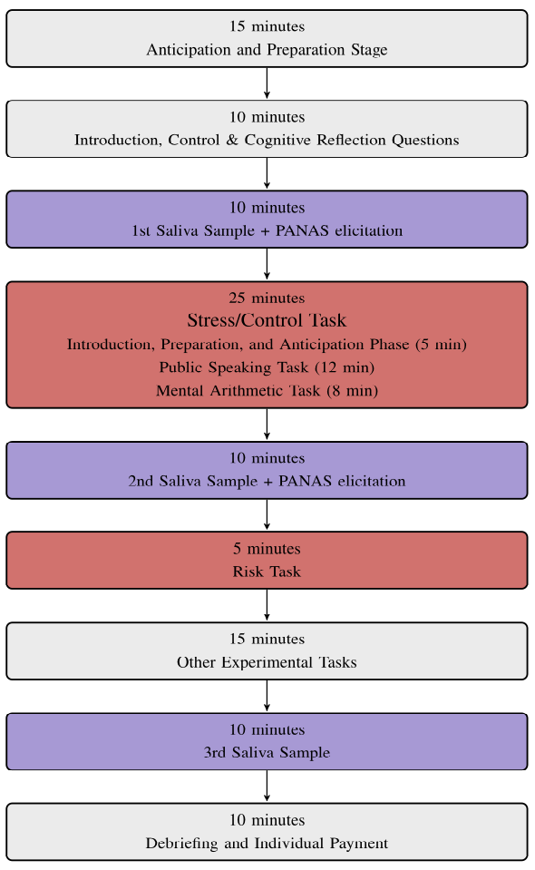
We conduct a laboratory experiment with 194 participants. The experiment has two main parts. For the first part, participants are randomized into one of two treatments: Stress or No-stress. The aim of this part is to induce stress among participants in the Stress condition. The second part is the same for all participants. In this part, we elicit individual risk attitudes. At several points, we collect information about stress levels. The timeline in Figure 1 provides a detailed overview of all the steps and the duration of each step.
In the first part, we expose participants to a task that is either stressful or not stressful. The task we use is the Trier Social Stress Test for Groups (TSST-G; Kirschbaum et al., 1993,von Dawans et al., 2011). It has been shown to reliably induce a significant stress response in approximately 70–80% of the treatment subjects in previous studies (DickersonKemeny, 2004,Giles et al., 2014), while the control condition has been shown not to induce stress (von Dawans et al., 2011,Het et al., 2009).
The main feature of the stress condition is that it involves a standardized performance task protocol, combining high levels of social-evaluative threat and uncontrollability in a group format with three phases:
For each session we invite at most 12 participants, six in each condition. For a detailed overview of experimental procedures and specific instructions, see section 3.4 and Appendix D, respectively.
In the Stress condition, participants are seated such that they directly face two neutral panel members, who are not involved in the other parts of the experiment as experimenters. Six chairs are placed in a row, separated by dividers such that subjects cannot see each other or communicate in any other way. The first five minutes are used to introduce the task to participants. After that, there is a public speaking task which lasts for 12 minutes, 2 minutes per subject. The TSST-G ends with a mental arithmetic task, where participants have to subtract numbers for six minutes, 1 minute per subject. To heighten the stress levels, the panel members wear white lab coats and have clipboards to take notes, and two video cameras are set up to film participants during the public speaking and mental arithmetic tasks.
The No-stress version of the TSST-G follows the same steps, with the following alterations. The panel members do not wear lab coats and are only present in the room without actively interacting with subjects, and there are no video cameras. Instead of the public speaking task, subjects are given a popular scientific text to read out aloud to themselves (all at the same time). Afterwards, subjects enumerate series of numbers in increments of 3, 5, 10, or 20 in a low voice from their individual seats for the same time duration as the mental subtraction task in the stress condition.
Stress levels are measured at different points during the experiment with the help of saliva samples (collected at three different moments as indicated in the timeline in Figure 1) and self-reported experienced stress levels (collected twice, using the PANAS scale; Watson et al., 1988).2 The different samples provide us with stress levels during the risk task as well as baseline levels that serve as a control.
The risk elicitation part of our study is based on a task developed by (Andersson et al., 2016). We opted for the method with a multiple price list (MPL) mainly because it allows us to detect and structurally estimate risk attitude parameters as well as errors in choices (manifested as reverse switches, i.e., switching back to the safer option after having chosen the riskier option once). It is important to emphasize that our analyses and arguments are based on the assumption that subjects have monotone preferences. Within this assumption, the level of consistency in choices serves as our measure for noise, and reverse switches are not consistent with monotone preferences. This assumption is not very restrictive, and allows to analyse results in a descriptive way without making many assumptions on the shape of a particular utility function for the descriptive analyses.
Popularized by (HoltLaury, 2002), MPLs are still one of the most widely used elicitation techniques for individual and aggregate risk preferences. The main two differences to the standard task by (HoltLaury, 2002) are that (a) the probabilities for both lotteries to decide between are fixed at p = 0.5 for the respective options, and (b) there are two separate MPLs to determine the overall risk attitudes.
Keeping the probabilities fixed has the advantage of not having to account for the possibility of subjective probability weighting. Also, it adds to the comprehensibility of the lotteries to depict them as a fair coin toss, labelling the options as Heads and Tails. This is a key feature of our design, since we want to minimize the possibility of observing noise due to confusion or the inability to calculate expected outcomes in subjects already by task design. A clear and comprehensible task ensures that our baseline measure itself is as unbiased as possible.
Using two separate MPLs allows to vary the switching point from the safer option to the riskier option - usually, price lists are designed that a risk neutral expected utility maximizer switches at the midpoint. The disadvantage of using two lists is that the midpoint also serves as a focal point, so that choices might not always reflect true preferences.
The specific lotteries are shown in 2. Note also that a risk neutral participant should switch relatively early in MPL1. This is an important feature of the design. As we argued before, apparent changes in risk attitudes can mask increases in errors. A very risk averse participant should switch only when the risky lottery becomes very attractive. This means that there is not much scope to make errors in the direction of switching ‘too late’. If stress increases noise, then for such a person it would appear as if they become less risk averse (they would sometimes switch too early and cannot switch too late, so on average the switching point is earlier).
Table 2: Risk Elicitation Task.
MPL 1 MPL 2 LEFT RIGHT LEFT RIGHT Dec. # HEADS TAILS HEADS TAILS HEADS TAILS HEADS TAILS 1 30 50 5 60 25 45 2 40 2 30 50 5 70 25 45 2 50 3 30 50 5 80 25 45 2 55 4 30 50 5 90 25 45 2 60 5 30 50 5 100 25 45 2 65 6 30 50 5 110 25 45 2 70 7 30 50 5 120 25 45 2 75 8 30 50 5 140 25 45 2 95 9 30 50 5 170 25 45 2 135 10 30 50 5 220 25 45 2 215 Note: This part of the experimental design is analog to (Andersson et al., 2016). The experimental currency are Token; the exchange rate to Euro is 1 Token = 0.20 Euro. One out of the 20 choices is selected at random at the end of the experiment and paid out in cash according to the exchange rate.
In the experiment, subjects are presented with one of the choice lists at a time (the order in which the lists are shown is randomized across subjects). Then, each row of the list is shown separately, in a random order within one list, and the subject makes a decision before moving onto the next randomly selected row, with a one second wait between each decision. We choose to have each choice presented on a single screen to make a midpoint of the list as a switching point less salient. However, this could naturally lead to an increased number of mistakes, which we counterbalance with the one second wait time to make subjects aware of the distinct decisions. Again, we rely on the simplicity of the overall task design, with only one variable changing on each screen within one list.
The currency of the values included in Table 2 is given in experimental tokens and converted to Euro at a fixed exchange rate of 1 Token = 0.20 Euro. At the end of the experiment, one of the 20 decisions is selected at random for each subject and paid out in cash according to the exchange rate.
There is no feedback given to subjects during the risk task. The only feedback subjects receive about the task is when they are informed about their payments on the final screen of the experiment, where they learn what the payoff-relevant decision situation was and the outcome of the respective lottery according to their choice.
We collected standard demographic measures such as age, gender, and field of studies. We also administerd a version of the cognitive reflection test (CRT; Frederick, 2005). Previous research has found cognitive ability to be correlated with the propensity to make errors (Andersen et al., 2006,HuckWeizsäcker, 1999,Dave et al., 2010). We used the version by (Toplak et al., 2014). It includes four questions and shows the same correlation with other cognitive measures as the original task, but is less familiar to subjects. The questions can be found in Appendix D.4. The test was administered before the stress induction (see the timeline in Figure 1), since otherwise stress could also impact the responses to this task.
For each session we invited up to 12 participants, 6 for the No-stress and 6 for the Stress condition. The maximum group size was set such that the stress levels would peak during the time that we elicited risk attitudes. The highest stress levels normally occur in the window of 35 to 45 minutes after the start of the TSST (Goodman et al., 2017).
Upon entering the lab, subjects were provided with magazines and asked to sit quietly and relax for about 15 minutes. After this, subjects were randomly assigned to either the No-stress or Stress condition, and led to separate rooms. Each room had six chairs placed in a row, separated by dividers such that subjects cannot see each other or communicate in any other way. Subjects wore noise-blocking headphones during the task whenever it is not their turn to speak, in order to standardise the task as much as possible. Two neutral panel members were seated directly facing the subjects.
The panel members were hired by the experimenters and this was known to the other participants. They had a strict protocol to adhere to and only gave neutral feedback throughout a session. We hired 3 male students and 1 female student. To avoid that results were driven by specific panel members or the gender composition of the panel, each panel member was randomly assigned to either the stress or low stress condition and this randomization was done at the session level.
The experiment was conducted at the University of Amsterdam. The eligible population for the study is economics and law students from the University of Amsterdam. The risk elicitation task as well as all additional measures (CRT, PANAS scale, demographics) were programmed in oTree (Chen et al., 2016). Written instructions are given to subjects and were read aloud to all participants by the experimenters (panel members in case of the TSST-G task, see section 3.1). Brief descriptions and explanations were given on screen during the tasks. Since our study deviated from standard economic laboratory experiments, we used strict exclusion criteria and preparatory instructions (to be adhered to one day before the actual experiment) for participants. Detailed information about the respective exclusion criteria, procedures, as well as instructions and task details are provided in Appendix A.3
Since cortisol follows a diurnal rhythm, for example producing a peak after waking and declining throughout the day, we ran 1 to 3 sessions per day of approximately 2 hours duration each at fixed starting points. The first session always runs 10–12, then 13–15, and the last session runs 16-18.4 In total, we ran 19 sessions with a number of participants between 6 and 12, depending on the respective show-up. However, we decided not to include the results of one of the sessions that we conducted (the 6th session out of 19) due to a disruptive participant during the stress treatment, resulting in a total of 18 sessions for the analysis. However, we include the ex-post analyses of the session with the disruptive participant as a robustness check in section F.1 in the appendix. We show that the results are robust to including these participants.
In this section we present the results for the pre-registered analyses of the experiment, including manipulation checks of the stress response, results of the risky choice task, and the exploratory analysis. We use two-sided independent samples t-tests for all of the analyses unless stated otherwise. In addition, we define a statistically significant effect as p < 0.005 and suggestive evidence of an effect as p < 0.05, following the recent proposal by (Benjamin et al., 2018). With our sample size of 194 participants, we have 90% power to find a Cohen’s d effect size of 0.47 (which represents a medium effect) with p = 0.05, and 90% power to find a Cohen’s d of 0.6 with p = 0.005.
In addition to the frequentist analyses we specified in our pre-analysis plan, we also present results of Bayesian analyses for our main results to be able to give a more conclusive interpretation of our data. All these analyses are done in JASP (JASP Team, 2022), for all Bayesian independent samples t-test we conducted we used the default Cauchy priors centered around zero with a scale of 0.707. This means that we expect the effect size to be between –2 and 2 with a probability of 80%, and 50% of the probability mass is on an effect size of −0.707 < δ < 0.707 . For the Bayesian linear regressions we used Jeffreys-Zellner-Siow (JZS) priors with an r scale of 0.354, and as the model prior we use a beta binomal distribution with Beta(1,1). The JZS prior assigns a Cauchy distribution centered around zero to each regression coefficient, with the same properties as for the independent samples t-test. The r scale as specified for the JZS prior is half the interquartile range of the Cauchy distribution, and as such corresponds to a scale of 0.707 as specified in the independent samples t-tests. The model prior specifies the prior likelihood of each of the estimated models. In contrast to a uniform prior, this prior assigns a higher prior probability to the model where both the treatment and other predictors are included in the regressions, instead of assuming equal plausibility of all models.
We decided to use the default priors in all our analyses here, since the previous literature is inconclusive on results and inconsistent in methods, so that we did not want to make any specific assumptions for priors based on previous data in a particular direction. However, the studies presented in table 1 in the literature review show that while several studies, for some sub-groups, do find a (slight) increase in risk taking, the majority of findings are inconclusive or report null effects. This also supports the choice of a prior centered around 0, while still allowing for larger effect sizes, with 20% of the prior mass on effect sizes below –2 and above 2, respectively. In addition, the defaults as specified above have desirable statistical properties (see general explanations in Keysers et al., 2020,Andraszewicz et al., 2015, and references therein), such as putting the main weight of expected effect sizes around 0, and also specifying that smaller effect sizes are more likely than larger effect sizes (in the default setting, 50% of the probability mass is on an effect size of −0.707 < δ < 0.707 ).
In total, 194 subjects participated in our study, 97 in the No-stress and 97 in the Stress condition, respectively. The majority of subjects came from the fields of economics, business administration, and finance (78.32%).5 A detailed overview of the composition of our sample can be found in Table 3. The rate of adherence to our pre-experimental measures can be found in the Appendix in Table 3. The mean age of subjects was 20.77 years. Sessions lasted for two hours including the payout of subjects, which was € 16 on average. On average, 29.27% of our female sample used hormonal contraceptives. Despite our aim to not have students with a psychology background participate, since they might be familiar with the task, we had roughly 20% psychology students in our sample.
Table 3: Descriptive Statistics — Subject Characteristics. The table gives an overview of the main demographic characteristics of the subject sample as well as the percentage of subjects using hormonal contraceptives if identified as female. This is important since hormonal contraceptives can impact the biophysical stress response in the body. Standard deviations for the subjects’ age are in parentheses.
All No-stress Stress Subject age 20.77 20.87 20.68 (2.49) (2.48) (2.51) Male 55.67% 53.61% 57.73% Contraceptive (if female) 28.24% 27.27% 29.27% Field of Study Economics 47.42 % 43.30 % 51.55 % Business administration 21.65% 25.77 % 17.53% Law 4.64% 5.15 % 4.12 % Finance 8.25% 9.28 % 7.22% Psychology 18.04 % 16.49 % 19.59%
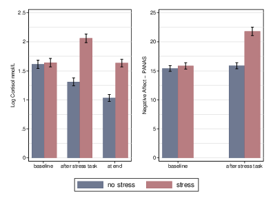
The left panel of Figure 2 shows the average cortisol measurements (in logs) of the Stress and no stress groups across the three sampling times. The results support the effectiveness of our stress manipulation. As expected, baseline levels of cortisol were very similar across groups, and not statistically different (p = 0.786). Participants in the Stress condition showed an increase in average cortisol levels right after the TSST-G, while the control group showed declining cortisol levels over the three measurement times.6 After the stress task, cortisol levels were substantially higher among participants in the Stress compared to the no stress group, and the difference is highly significant (p < 0.001).
 (a) cortisol measurements (b) negative affect scale
Figure 2: Average log cortisol measurements and self-reported negative affect by treatment. This figure depicts the average log cortisol measurements across treatments Stress and No-stress across the three sample time points in the left panel (a). The right panel (b) shows the negative affect score of the PANAS scale at the baseline and right after the stress task across treatments. The bars represent standard errors.
However, only a comparatively low fraction of 52.69% of subjects actually exhibited a cortisol response.7 Following the literature, we define an active cortisol response using a threshold of a 1.5nmol/L baseline-to-peak increase (Miller et al., 2013) (equivalently, a percentage increase of at least 15.5% for Time 2 compared to Time 1). A cortisol nonresponse is therefore an increase in cortisol less than this. As additional information, we present an overview of the summary statistics of all compliance measures (such as not drinking coffee prior to the experiment on the day itself, brushing teeth before coming to the lab, etc.) in section E.1 in the appendix. Almost all subjects complied to our measures, which does not explain the comparatively low percentage of subjects exhibiting a cortisol response in our treatment.8
In the appendix, we include pre-registered regressions controlling for the session time and oral contraceptive (OC) use in females on cortisol reactivity (appendix E.2). We found no evidence that either of the two factor affected cortisol reactivity.
For our second manipulation check, we present the results of the two self-assessed stress measures of the PANAS (at the beginning of the experiment and right after the TSST-G), see the right panel of Figure 2. We use the negative affect score as an indication of the individually perceived subjective stress levels and compare the respective scores between treatments. We therefore calculate the difference in negative affect score for each subject as the score elicited right after the TSST-G minus the score at the beginning of the experiment.
Participants in the Stress group had significantly higher negative affect score relative to the baseline on average compared to the control group participants (p <0.001, N= 194). This provides evidence that our stress treatment created subjective feelings of stress for the Stress group relative to the control protocol.
In sum, both subjective and objective measures of stress show that the stress manipulation was effective.
We first analyze the number of safe choices made by an individual, and the number of times that the person switched from the risky option (back) to the safer option, where the latter is our first measure of noise. This noise index can vary between 0 and 10. Table 4 presents an overview of the main variables of interest, which are the mean number of safe choices overall and across treatments, as well as an overview of the mean CRT scores as a proxy for cognitive abilities. The latter is important since we want to make a claim about a negative correlation of cognitive abilities and noise in general, and in particular a disproportional effect of stress on observed noise for subjects with lower cognitive abilities. Therefore we check for successful randomization across groups, and with a mean number of correctly solved questions of 2.16 and 2.36 out of 4 questions overall in the No-stress and Stress conditions, the difference is not statistically significant with p = 0.273.
Table 4: Descriptive Results — Means. Standard deviations are in parentheses. p-values are obtained using two-sided t-tests. The total number of possible safe choices was 20 (for all of the decisions in the two multiple price lists); the maximum number of reverse switches is therefore 10.
All No-stress Stress p-value Number of safe choices 12.92 12.67 13.16 0.30 (3.33) (3.30) (3.37) Number of reverse switches 1.81 1.99 1.63 0.22 (2.03) (2.11) (1.94) CRT score 2.26 2.16 2.36 (1.24) (1.25) (1.23) 0.27
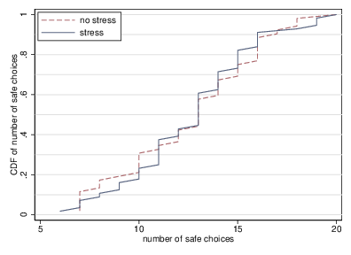
Figure 3 graphically presents differences across conditions including 95% confidence intervals (left panel), and also gives an overview of the actual distributions plotting the cumulative distribution functions (right panel). The latter adds more detailed information about the actual distributions of the number of safe choices across conditions, rather than only informing about (differences in) means. Across both conditions, we observe risk averse choice behavior on the aggregate. A risk neutral subject would choose the safer option seven times (two times in MPL 1, five times in MPL 2, as described in section 3.2 in detail). On average, subjects in the No-stress condition chose the safer option 12.67 times (63.4%) out of 20 choices in total, whereas subjects in the Stress condition chose the safer option 13.16 (65.8%) times. The difference in the mean number of safer choices between conditions is not statistically significant with p = 0.302 (Table 4, first row). We found no conclusive evidence that stress affects choices, at least at the aggregate level.
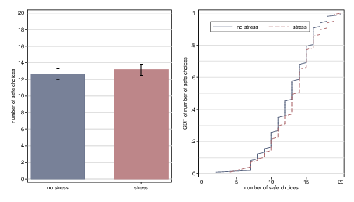
Figure 3: Mean number of safe choices across conditions. The left panel of this figure depicts the mean number of safe choices in the no stress (red) compared to the Stress (blue) condition. The mean number of safe choices is calculated using both lists in the risk task. The error bars represent the 95% confidence intervals. The right panel of this figure presents the cumulative distribution functions of the number of safe choices across treatments. The blue line represents the no stress condition, the dashed red line represents the Stress condition.
To get a more conclusive insight, we present the results of Bayesian analyses. The results reveal that with a BF01 = 3.890 (Bayesian independent samples t-test), the data is 3.890 times more likely to be observed under the null hypothesis (which is that the mean number of safe choices is the same across treatments) and thus provides substantial evidence for the null. This strengthens our findings of the frequentist analysis, where we did not find a significant difference in the mean number of safer choices. To address our first hypothesis as stated in the introduction, where we expected that risk taking increases under stress, the results show that with a BF0+ = 12.209 (Bayesian independent samples t-test) the data is 12.209 times more likely under the null hypothesis — the mean number of safe choices is the same across groups — compared to the alternative hypothesis that the mean number of safer choices is lower under stress, providing strong evidence for a null effect.
Overall, we do not find evidence for our hypothesis H1, where we expected that risk seeking increases under stress. We address different specific types of noise later in our parameter estimations in section 4.4, where we estimate noise and risk attitudes jointly.
Choosing the safer option can be driven by underlying risk attitudes or by noise in the decision-making process. To capture noise, we count how often a subject switches back to the safer option, after having switched from the safer to the riskier option. Naturally, a rational decision maker switches at most once from left to right (from a "safer" to a "more risky" lottery). Whenever a subject switches back, we count this as noise. Consequently, if a subject switches at most once, our noise measure has value 0. If a person switches 5 times starting from the safer option, our noise measure has value 2 (the person switched back twice to the safe option). We refer to this number as the number of reverse switches.9
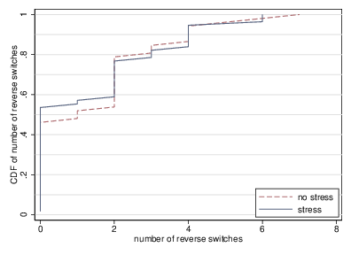
Using this measure of noise, Figure 4 shows noise by condition. We find no evidence that stress increases noise. Out of a maximum of ten, subjects in the No-stress treatment switch back 1.99 times, against 1.63 reverse switches in the Stress condition. Thus, if anything, it seems that behavior becomes less noisy under stress. However, the difference is not statistically significant given our two-sided test (p = 0.217).
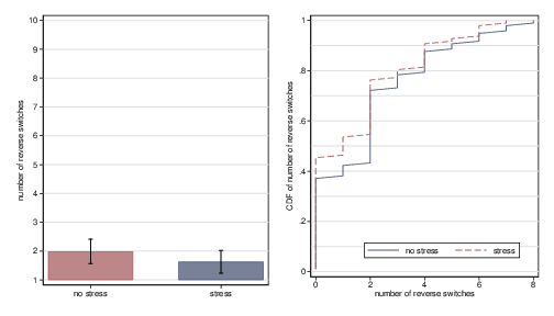
Figure 4: Mean number of reverse switches across conditions. The left panel of this figure depicts the mean number of reverse switches in the No-stress (red) compared to the Stress (blue) condition. The mean number of switches is calculated using both lists in the risk task. The error bars represent the 95% confidence intervals. The right panel of this figure presents the cumulative distribution functions of the number of reverse switches across treatments. The blue line represents the no stress condition, the dashed red line represents the Stress condition.
Again supplementing these findings with Bayes factors, we first present the analogue to our two-way independent sample t-test: with BF01 = 3.136 (Bayesian independent samples t-test) we find that the data is 3.136 times more likely to be observed under the null hypothesis (no difference in the noise observed across conditions) compared to the alternative hypothesis that there is a difference in the noise observed across conditions, which constitutes substantial evidence in favor of the null hypothesis. Addressing our hypothesis as stated in the introduction, with a Bayes factor of BF0+ = 13.472 (Bayesian independent samples t-test) it is 13.472 times more likely to observe the data we obtained under the null compared to the alternative hypothesis, where the latter states that there is a higher level of noise under stress, constituting strong evidence in favor of the null hypothesis.
Taken together, we find strong evidence that there is no difference in the observed levels of noise across conditions. Overall, we do not find evidence for our hypothesis H2, where we expected that noise increases under stress.
In a next step, we regress the number of reverse switches on stress and CRT scores, results are displayed in Table 5. CRT scores have been shown to be negatively correlated with noise in decision-making (see, e.g., Andersson et al., 2016). Controlling for CRT scores does not affect the coefficient of stress. We do indeed observe that a higher CRT score is associated with fewer switches. In column (3), we include an interaction term between Stress and CRT. The effect of stress remains insignificant and the interaction term is small, indicating that stress does not have a differential effect across groups with different CRT scores. As pre-registered in our analysis, we conduct Ordered Probit regressions to account for the categorical nature of the outcome variable. These results can be found in appendix E.3, results remain qualitatively unchanged.
Table 5: OLS regression results. This table shows the coefficients for the regression of treatment (Stress) and cognitive abilities (CRT) on the number of reverse switches across both choice lists in risk task. Bootstrapped standard errors are in parentheses. We had 18 sessions in total, with 6 to 12 participants in each session. Stars indicate significance levels, * p < 0.05; ** p < 0.005; *** p < 0.001.
Number of reverse switches Stress CRT Stress x CRT Constant N R2
In Table 6 we provide the results of a Bayesian linear regression to support our results further. The results show that our data is most likely under the model with CRT as the only predictor of the number of reverse switches across treatments with a posterior probability (probability this model is best explaining the data after having observed the data) of 0.538. In addition, our data is 2.959 times more likely under the model with CRT as the only predictor compared to the model including the combination of treatment and CRT, which constitutes anecdotal evidence in favor of the CRT only model.
Table 6: Bayesian Linear Regression: Model Comparison. This table shows the results for a Bayesian linear regression of treatment (Stress) and cognitive abilities (CRT) on the number of reverse switches across both choice lists in the risk task. P(M) denotes the prior probability for each model, where we use a Beta(1,1) distribution as the model prior. P(M|data) is the posterior probability for each model.
Dep. variable: Number of reverse switches Models CRT Stress + CRT Null model Stress
In particular, we find partial support for our hypothesis H3: whereas we find that lower cognitive abilities are related to significantly more errors in decision-making, stress in itself does not increase observed noise.
Summing up our results so far, we do not find that subjects display more risk seeking (or risk averse) behavior under stress. Since we do not detect an effect on noise, this suggests that the underlying preferences must be largely unaffected by stress. Both of those conclusions drawn based on frequentist analyses are supported by Bayes factors as well as Bayesian linear regressions. Bayesian analyses suggest strong evidence for a true null effect, supporting the stability of aggregate preferences across treatments and, in contrast to our predictions, no increase in observed noise in the Stress condition.
In this section we provide structural estimates of the risk-aversion and noise parameters. Compared to simply counting the number of safe choices and number of switches, this allows for a more direct test of the effects of stress on underlying risk attitudes, addressing our hypothesis H1. This comes at the expense of having to make more assumptions about the utility function and the type of errors that subjects make.10
We follow the approach of (Loomes et al., 2002) and divide the decision itself into a three-step process, where we focus on stages two and three. The first step is the preference selection stage, where subjects identify their current preference. The second step is the stage where prospects are evaluated, which, in our case, corresponds to the calculation of the expected outcomes of the lotteries. The type of error that occurs in this stage is the so called “Fechner” error, popularized by (HeyOrme, 1994). The third step is the stage where subjects finally act and make a decision. In our case this is clicking the mouse to submit one out of two options. The type of error that occurs here is a “trembling hand” error, put forward by (Luce, 1959).
In our estimations, we first present the results of a model which does not account for errors separately. Second, we introduce the Fechner error specification, followed by the trembling hand error specification. In a last step, we combine both Fechner and trembling hand errors. By doing so, we can both quantify the observed inconsistencies and meaningfully compare treatment differences. In the following, our analyses rely on (Harrison et al., 2007) for the most part.
Assuming a CRRA functional, utility over money is defined as:
| u(x) = xr, (1) |
where r is the utility function curvature parameter to be estimated, x denotes the respective outcome amounts of the lottery. r = 1 corresponds to risk neutrality, r < 1 indicates risk aversion, and r > 1 risk seeking preferences. For outcomes k=1,...n, the expected utility (EU) is then given by:
| EUi = |
| [pk × uk]. (2) |
The EU difference is calculated for a candidate estimate of r by taking differences of the two lotteries to choose from in our experiment (L for left lottery, R for right lottery):
| Δ EU = EUR− EUL (3) |
This latent index, which is based on latent preferences, is linked to observed choices using a standard normal distribution function Φ (Δ EU). This probit link function takes any argument between ± ∞ and transforms it into a number between 0 and 1:
| Prob(choose lottery R) = Φ(Δ EU) (4) |
Since we do not allow for indications of indifference in our experimental task, the conditional log-likelihood assuming EUT with a CRRA functional framework and a cumulative density function in the probit framework is:
| ln L(r;x, X) = |
| ((ln Φ (Δ EU) | yi = 1) + (ln Φ(−Δ EU)|yi = −1)) (5) |
yi = 1 denotes the choice of Option right, yi = − 1 denotes the choice of Option left in the lottery in our risk task decision i, X is a vector of individual characteristics.
Specifying this via a maximum likelihood program, we obtain the structural estimate for r. We then test for differences between our No-stress and Stress conditions via standard post-estimation Wald-tests. Additionally, we control for multiple responses from a single subject (each subject has to make 20 decisions in total) by clustering standard errors on the individual level.
Taking the baseline model as a starting point, we now augment this model by allowing for probabilistic errors. In other words, this model allows subjects to make some errors in their decisions in the risk elicitation task.
The first specification we use is a framework established originally by Fechner, popularized by (HeyOrme, 1994). Due to this specification, errors happen at the stage of actually making the decision. Adding a noise term to the latent index specification of the baseline model in 3, we have:
| Δ EU′ = EUR − EULµ (6) |
µ is used to allow errors from the perspective of the deterministic EU model. According to the model specification, the errors happen at the evaluation stage of the expected utilities of the Heads and Tails option. Thus, the index Δ EU′ is in the form of a cumulative distribution function defined over differences in the EU of the right and left option as well as the noise parameter µ.
The second error specification we use is based on (Luce, 1959) and also used by (HoltLaury, 2002). For this matter, we use the ratio form introduced above by calculating the EU for each lottery pair for candidate estimates of r, adding a structural noise parameter ω:
| Δ EU″ = |
|
| (7) |
Otherwise using the same steps as in the baseline model, we can estimate the Luce error specification with maximum likelihood methods again, accounting for heteroscedasticity and clustering SEs on the individual level.
The results for the structural estimations of the four model specifications are provided in Table 7. The first three columns present the results for the model without any error specification, the middle three columns show results obtained by the Fechner error model, and the right three columns then for the constant error model (Luce, 1959). All p-values are obtained via post-estimation Wald tests unless mentioned otherwise.
Table 7: Parameter estimates for utility function curvature and an error parameter. This table shows the parameter estimates for the utility function curvature as well as the parameter estimate for choice errors. All parameters are obtained via maximum likelihood estimations using the Broyden-Fletcher-Goldfarb-Shannon (BFGS) optimization algorithm. The left three columns include estimations without an error specification, the middle three columns include estimations obtained via the Fechner model, and the right three columns include estimations obtained via the Constant error model. Standard errors are clustered on the individual level. All p-values are obtained via post-estimation Wald tests.
Without errors Fechner model Constant error model No-stress Stress p−val. No-stress Stress p−val. No-stress Stress p−val. 0.471 0.463 0.596 0.442 0.413 0.375 0.469 0.436 0.359 (0.010) (0.011) (0.023) (0.023) (0.026) (0.025) 0.454 0.382 0.379 (0.062) (0.052) 0.100 0.094 0.600 (0.007) (0.008) –860.9 –861.4 –852.1 –842.1 –840.7 –835.3 For all models, there were 97 clusters, N was 1,940.
Across all specifications, estimated parameters for utility function curvature indicate risk aversion with α < 1, confirming descriptive results, together with a slightly higher degree of risk aversion under stress. The differences between the No-stress and Stress conditions are not significantly different for either of the columns (p > 0.375). With respect to the estimated noise parameters under No-stress and Stress, we find that Fechner errors are not significantly different across specifications (p = 0.379), which is similar for the tremble specifications (p = 0.600).
Overall, we find that errors do not increase under stress as also confirmed by the estimation results.
In addition to our pre-registered analyses presented above, we include an exploratory section where we zoom in on a potential differential effect of stress on risk taking on male and female participants. This is based on the findings of the previous literature on gender differences in risk attitudes in general (see EckelGrossman, 2008,CrosonGneezy, 2009,CharnessGneezy, 2012, for example) and the findings in the domain of stress and risk taking in particular (see from the literature overview in Table 1).11 It is important to note that we are analyzing treatment effects within male and female sub-samples, but do not compare differences in treatment effects across sub-samples. We therefore refrain from making a claim about whether those treatment effects for female and male participants are significantly different.
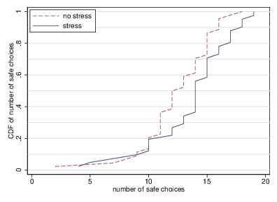
Figure 5 shows the cumulative density functions of the number of safe choices between treatments for male (left panel) and female (right panel) participants. For male participants, the density functions for the Stress and no stress conditions almost overlap, and the differences in distributions are not significant (p = 0.941 , N = 108, Mann-Whitney U test). However, females appear to make a higher number of safe choices under Stress, which is also statistically significant (p = 0.038, N = 85, Mann-Whitney U test).
male female
Figure 5: Mean number of safe choices across conditions - gender differences. The left panel of this figure presents the cumulative density functions of the number of safe choices across treatments for male, the right panel for female participants. The blue line represents the no stress condition, the dashed red line represents the Stress condition.
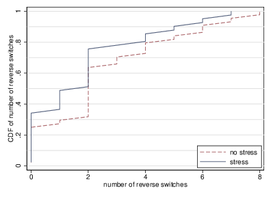
To account for a potential difference in noise across conditions and gender, we present the cumulative distribution functions for the number of reverse switches in Figure 6. There are no significant differences in the number of reverse switches across stess and no stress conditions in either the male or female subsample ( p = 0.660, N = 108 - male; p = 0.128, N = 85 - female; Mann-Whitney U tests).
male female
Figure 6: Mean number of reverse switches across conditions - gender differences. The left panel of this figure presents the cumulative density functions of the number of reverse switches across treatments for male, the right panel for female participants. The blue line represents the no stress condition, the dashed red line represents the Stress condition.
This additional analysis shows that it might indeed be important to zoom in on potential differential effects of stress on risk taking for male and female participants. The overall null effect of our analysis seems to mask an increased degree of risk aversion among female participants when under acute stress compared to the no stress condition.
Given the small sample size and the exploratory nature of the analyses, we want to be cautious in interpreting those results. To give more information and interpretation of the data at hand, we conduct additional Bayesian independent samples t-tests for the analyses presented above. For male subjects, the results reveal that with a BF01 = 4.886, our data on the number of safer choices is 4.886 times more likely to be observed under the null (no differences in the number of safer choices across treatments) than under the alternative hypothesis (differences in the number of safer choices), which constitutes substantial evidence in favor of the null hypothesis. We also find substantial evidence in favor of the number of reverse switches being equal across treatments with a BF01 = 4.759. For female subjects, the results look different: with a Bayes factor close to 1, we only find no evidence in favor of either the null or alternative non-directional hypothesis (BF01 = 1.099) for the number of safer choices as the outcome variable. For the number of reverse switches, we find anecdotal evidence in favor of the null hypothesis of no differences in the number of reverse switches (BF01 = 1.832).
Structural estimations point in the same direction as our earlier findings when splitting the sample in male and female participants, as presented in Table 8. For each of the models, we estimated all parameters for male and female participants separately. Results show that the estimations without including a specific model for errors do not support a significant higher degree of risk aversion for neither male nor female participants under stress as compared to no stress (p = 0.827 - male, p = 0.356 - female). For both the model with a Fechner and constant error model structure, women seem to be slightly more risk averse under stress with α = 0.448 in the no stress and α = 0.367 in the Stress condition in the Fechner model, and α = 0.476 in the no stress and α = 0.385 in the Stress condition in the constant error model. However, neither of those differences are statistically significant with p > 0.066. In the male subsample, the parameters are almost identical (α = 0.451 – no stress, and α = 0.450 – Stress, Fecher model; α = 0.476 – no stress, and α = 0.474 – Stress, constant error model) with p > 0.979.
Table 8: Parameter estimates for utility function curvature and an error parameter. This table shows the parameter estimates for the utility function curvature as well as the parameter estimate for choice errors. All parameters are obtained via maximum likelihood estimations using the Broyden-Fletcher-Goldfarb-Shannon (BFGS) optimization algorithm. The left three columns include estimations without an error specification, the middle three columns include estimations obtained via the Fechner model, and the right three columns include estimations obtained via the Constant error model. Standard errors are clustered on the individual level. All p-values are obtained via post-estimation Wald tests.
Without errors Fechner model Constant error model Utility parameter α Male 0.484 0.479 0.827 0.451 0.450 0.985 0.476 0.474 0.979 (0.014) (0.016) (0.034) (0.031) (0.037) (0.033) Female 0.463 0.444 0.356 0.448 0.367 0.069 0.476 0.385 0.066 (0.014) (0.014) (0.030) (0.033) (0.033) (0.037) Error parameter µ Male 0.428 0.442 0.894 (0.079) (0.075) Female 0.512 0.308 0.095 (0.100) (0.070) Error parameter ω Male 0.090 0.095 0.723 (0.007) (0.010) Female 0.111 0.090 0.270 (0.014) (0.013) # of clusters Male 52 56 52 56 52 56 Female 44 41 44 41 44 41 N Male 1,040 1,120 1,040 1,120 1,040 1,120 Female 880 820 880 820 880 820 Log likelihood Male –433.1 –478.3 –426.5 –471.6 –418.6 –466.4 Female –410.8 –378.7 –408.8 –363.4 –405.1 –361.9
In our study, we analyze the impact of experimentally induced stress on decision-making under risk in a pre-registered laboratory study with 194 subjects and find no significant differences in risk attitudes across treatments. In particular, our contribution to the literature is that we can account for noise in decision-making, and therefore isolate a true shift in preferences across treatments from a pure increase in noise. Not accounting for noise, this can lead to an over- or underestimation of the observed effect, as well as a biased baseline measure in itself.
We were able to successfully induce acute psychological stress in our treatment group, based on significantly increased cortisol reactivity in the treatment group on average relative to the control group. The same holds for subjectively reported feelings of negative affect. Taken together, on average, subjects showed a significant physiological and psychological stress response in the treatment group.
Our results across specifications show that there is no statistically significant impact of stress on risk preferences, supported by both parameter estimations and Bayesian analyses. Furthermore, we have evidence that this robust null result is not driven by increased noise in decision-making under stress. However, baseline levels of cognitive ability affect errors in decision-making, in accordance with previous literature (see, e.g., Andersson et al., 2016,Andersson et al., 2020). The statistically significant negative association between cognitive ability and decision errors does not appear to be isolated to the stress treatment, and in particular, stress does not have a disproportionate effect on decision errors of subjects with lower cognitive abilities. This is also supported by Bayesian linear regressions, where we find that our data is 2.959 times more likely to be observed under the model with cognitive abilities as the only predictor of the number of reverse switches compared to a model including both a treatment dummy and cognitive abilities, and even 40 times more likely compared to a model including a treatment dummy only.
In an exploratory analysis that was not pre-registered, we investigate whether there might be gender differences in risk taking under stress. This is based on the literature on gender differences in risk attitudes in general (see EckelGrossman, 2008,CrosonGneezy, 2009,CharnessGneezy, 2012, for example), and some significant findings for one gender but not the other in related studies analyzing stress and risk taking in particular (see from our literature overview in Table 1. Even though non-parametric tests find suggestive evidence that females seem to become more risk averse under stress, Bayesian analyses do not confirm this trend: we find no evidence in favor of either the null or the alternative hypothesis (i.e., a difference in the number of safe choices across conditions).
Our findings warrant some discussion given the findings of the related literature. As outlined in the literature review, there is no real consensus on in which direction the effects of stress on risk preferences go: 50% of the directly related studies find an increase in risk taking in the stress condition in at least one subsample of the participants, 37.5% an increase in risk aversion, and 93.75% no significant effect in at least one of the elicited dimensions (e.g., gains/losses) or among one of the subsamples (men/women, cortisol responders/non-responders).
Taken these findings and given our data, we presume that the small sample size of previous studies, with potentially severely underpowered results, is a first very likely contributor to an apparent change in risk attitudes across conditions. We conclude that those findings reporting a significant change in aggregate risk attitudes under stress, are not robust to replication and thus should be interpreted with caution.
A second potential candidate for the observation of apparent changes in aggregate risk attitudes under stress in some of the previous literature is not accounting for potential noise in decision-making. To isolate the effect of stress on risk attitudes for a causal interpretation of the treatment effect, we take two measures: First, we use a particularly simple task design, based on previous findings that such simple designs mitigate noise in decision making (Dave et al., 2010). A simple design as ours is characterized by relatively few decisions a subject has to make, and keeping probabilities fixed across decisions. Second, we account for different types of errors — Fechner errors and trembling hand errors — by using and comparing different parameter estimation strategies.
In particular, the features of our task design for eliciting risk attitudes becomes important when interpreting the results in light of the previous literature. The argument is based on (Dave et al., 2010): On the one hand, a simple task that requires little cognitive effort has the upside of observing less noise in subjects’ choices and thus provides a less biased estimate of subjects’ risk attitudes when using simple analyses, such as counting the number of safer choices. What makes a task comparatively simple is a relatively small number of decisions to make, and keeping probabilities fixed, so that decision situations only vary in outcomes. On the other hand, a simpler task design potentially comes at the expense of predictive ability — and as such, with a potentially lower internal validity. However, in an experiment where we can expect an increased level of noise in at least one of the treatments ex ante, a coarser but simpler measure is preferred. This is important when interpreting our results: we find little noise overall, and no significant increase in noise under stress. This, however, does not lead to the conclusion that noise is not the driver of the lacking consensus in the findings in related studies. In fact, the majority of related studies use complex choice tasks with that have been shown to produce high levels of noise in subjects’ decisions (Dave et al., 2010).
Another component that makes a direct assessment of the reliability of a number of related studies complicated are task designs that include varying probabilities and outcomes. In particular, varying probabilities can bias risk attitudes through non-linear probability weighting (see from WakkerDeneffe, 1996, for example), which is an additional source of potential variation under stress. Especially in complex task designs, it is hard to interpret whether an apparent change in risk attitudes stems from a bias induced by noise, probability weighting, or both, or whether it is a true difference in risk attitudes.
Adding to the points above, we briefly discuss the external validity of our results, or, in other words, in how far we can claim that our method of eliciting risky choices actually measure risk attitudes (see discussion in Frey et al., 2017, for example) and to what extent our results are generalizable. There is an ongoing debate about the external validity of laboratory measures of risk attitudes, given that even across laboratory measures of risk attitudes, individual attitudes have found to not be very strongly correlated (see also Pedroni et al., 2017, for example). However, a recent study shows that subjects are actually aware of the their apparent inconsistency in attitudes across choices (HolzmeisterStefan, 2021). This points to the interpretation that those tasks actually measure task-related risk attitudes that are not fully generalizable to all areas and specific situations of risk taking. However, we are interested in treatment differences, that is, whether there is any shift in preferences across stress and no-stress conditions. With this, we explicitly refrain from interpreting the absolute level of measured risk attitudes, both in the descriptive as well as the parameter analysis. In particular, we only make relative statements, comparing the attitudes in the condition under stress to the attitudes in the no-stress condition, characterizing attitudes as relatively more/less risk seeking, or stable.
As a last point, we want to mention that despite our aggregate null findings across conditions, there could be directions in opposite effects that overall lead to our null finding. In other words, both an increase in risk seeking and an increase in risk aversion could co-exist within our sample, and the overall average effect we observe is a null effect, cancelling out the effects going in opposite directions. We cannot account for this potential heterogeneity of the impact of stress on risky choices in our experiment. For a clean identification of those effects, a within-subject comparison is needed, which we cannot provide with our data.
Naturally, our experiment has several limitations to be addressed in further research. Given that we studied acute stress only, we acknowledge that chronic stress might have a stronger influence on shifting risk preferences, or that repeated episodes of stress could increase errors in decision-making unlike acute stress. Additionally, it could be the case that stress affects risk preferences in different directions based on individual characteristics, such as ability to cope with stress, and therefore average treatment effects may not capture this heterogeneity.
Since our study deviates from standard economic laboratory experiments, we have strict exclusion criteria for participants. In general, the eligible population for the study is economics and law students from the University of Amsterdam. From the pool of those students who registered for receiving invitations for experimental studies, we draw a random sub-sample getting access to signing up for our experiment. We do not invite subjects with prior participation in stress experiments due to a possible learning effect and therefore a lower reaction to our treatment. Due to our measurement of cortisol as a control for the success of our stress induction method, we have strict exclusion criteria even within this sub-sample. To be able to reliably test for a treatment effect in cortisol levels, subjects who have a potentially different baseline level or a decreased/increased expected reaction due to medical conditions are excluded from participation. These conditions include any regular medication intake (excluding oral contraceptives), pregnancy or breastfeeding, reported medical or psychiatric/neurological illness/disorder, substance abuse, daily use of nicotine, and self-reported severe stress. Additionally, since gum/oral problems like bleeding might lead to a distorted measurement of cortisol, we also have to exclude these subjects. Since the experiment is conducted in English, fluency in the English language is required.
All exclusion criteria are:
On the day prior to and the actual day of the experiment, we required subjects to follow some preparation instructions. We asked subjects not to eat (including chewing gum), take nicotine, or drink anything but water, two hours prior to their session time. Additionally, brushing teeth after the last meal and at least one hour prior to the session time was required for an uncontaminated saliva sample. The day before and the day of the subjects’ session time, we required them to avoid alcohol, exercise, caffeine and any medication such as painkillers (excluding oral contraceptives). Participants were asked to ensure that normal meals are consumed. On the day of the experiment, we instructed them to be awake from at least 3 hours prior to their session time.
All preparatory details:
E-Mail reminders are sent to subjects one day prior to the actual experiment.
We invite you to participate in an economics lab experiment involving a challenge task, and a series of decision-making tasks on a computer. Parts of the test session may include videotaping. The session will take approximately 2 hours.
At certain points in the experiment, the physiological responses of your body will be measured using standard procedures. For this reason, we ask that you do not eat (including chewing gum), take nicotine, or drink anything but water two hours prior to your session time. Please brush your teeth after your last meal and at least one hour prior to your session time.
The day before and the day of your session time, we require you to avoid alcohol, exercise, caffeine and any medication such as painkillers (excluding oral contraceptives). Ensure that you are eating meals as normal. Please also ensure that you are awake from at least 3 hours prior to your session time.
Compensation: Those who arrive on time will receive a 7 Euro show up fee. In addition, participants will have the opportunity to earn up to an additional 44 Euros, depending on their choices. There is the possibility that some subjects will be turned away from the experiment. Those who are turned away will receive the show up fee and will not be required to stay for the study.
Eligibility requirements: No psychology courses taken at university level, (if female) not currently pregnant or breastfeeding, not currently taking any medications (excluding oral contraceptives), fluent in English, no current medical illness, no daily nicotine (such as cigarettes) usage, no present or past psychiatric or neurological disorder, not currently under severe stress (such as exam stress), able to abstain from caffeine, no oral health/gum issues (such as bleeding), no substance abuse, no regular drug taking.
This scale consists of a number of words that describe different feelings and emotions. Read each item and then list the number from the scale below next to each word. Indicate to what extent you have felt this way in the last 10 minutes.
Positive Affect Score: Add the scores on items 1, 3, 5, 9, 10, 12, 14, 16, 17, and 19. Scores can range from 10 – 50, with higher scores representing higher levels of positive affect.
Negative Affect Score:
Add the scores on items 2, 4, 6, 7, 8, 11, 13, 15, 18, and 20. Scores can range from 10 – 50, with lower scores representing lower levels of negative affect.
Dear participants,Welcome to today’s experiment and thank you very much for your participation!
General Procedure
This is an experiment about decision-making. You will be paid for participating, and the amount of money you will earn depends on the decisions that you make. At the end of the experiment you will be paid privately and in cash for your decisions.The entire experiment will take at most 1 hour and 45 minutes and consists of several parts. You will receive detailed instructions at the beginning of each part. In case you have any questions after having read the instructions or during the experiment itself, please raise your hand. One of the experimenters will come to your cubicle and answer your questions privately.
During the entire experiment, you are asked to make decisions. Your decisions as well as chance can determine your payment. The payment will be calculated according to the rules as described in the following parts. Please read through the instructions carefully. All information provided in the instructions are truthful. The amount of your payment at the end of the experiment also depends on how well you were able to understand the instructions.
Payment
You will receive a fixed amount of EUR 10 for your participation in the whole experiment. For some parts of the experiment, you can earn additional money. In the respective parts of this experiment, your payment will either be displayed in Euros or in Tokens. Your possible payouts as well as the conversion rate from Token to Euro will be explained in detail in the instructions of the respective part. At the end of the experiment, we will display your final earnings on screen.
Your Identity
You will never be asked to reveal your identity to anyone during the course of the experiment. Your name will never be recorded by anyone. Neither the experimenter nor the other subjects will be able to link you to any of your decisions.In order to keep your decisions private, please do not reveal your choices to any other participant.
Other
We kindly ask you to refrain from talking to any other participants and only use the aids provided by the experimenters. Please turn off your electronic devices. You are not allowed to use them at any point during the experiment. You are only allowed to use computer functions that are necessary for the experiment. In case of any rule violations, you will not receive any payment for this experiment and be banned from participation in future experiments.Thank you very much for your attention and your participation in today’s experiment.
All 12 subjects per session begin in the experiment room.
The experiment room consists of an open area in the back with rows of computers in the front. The room will be set up with two chairs at the back for the stress panel members to sit at, as well as a row of 6 chairs with dividers in between for the stress subjects to sit at. The panel members will wear lab coats and they will have clipboards to use for taking notes, and there will be video cameras to film the subjects under the stress condition only. There will also be a panel in the control condition but the subjects will not be filmed. We instruct subjects not to talk to each other throughout the entire experiment.
First there is an acclimation period of 15 minutes in which subjects sit calmly and quietly to ensure the baseline cortisol level will be taken in a non-stressed state. They are given neutral texts to read, e.g., magazine, while sitting in their individual cubicles. At the end of this 15-minute rest period they begin the experimental procedure on the computer by filling out their details, answering the pre-experiment questionnaire and control questions. Then they answer the first PANAS survey. Then they are instructed how to take a saliva sample and they take the first sample to get the baseline measurement. (pre TSST-G period is 30 minutes)
There is a second room next to the experiment room where the control group will undergo the control version of the TSST-G while the treatment group undergoes the TSST-G in the experiment room. We will have performed a randomisation before the subjects enter the experiment room to determine which half of the group is treatment and which is control. The control group will move into the adjacent room now.
Then, depending on whether the group is treatment or control, they will follow either the stress or control protocols.
Panel members: in each panel we will have two people. We will recruit 3 male students and 1 female student (we could not get a gender balance due to resource issues) for this task so that we attempt to have the same people throughout the whole experiment. We will randomly allocate the panel members to either the treatment panel or the control panel across sessions. All feedback in the stress protocol should remain neutral throughout the session (both verbal and nonverbal).
The panel enters the room, participants are informed that the panel members will observe them and that they will be filmed.
The stress treatment protocol consists of two tasks: a public speaking part and a mental subtraction part. Participants sit in a row separated by dividing screens (so they cannot see the other participants) and are selected in random order to perform each task (one task at a time).
Begin with a 5 minute instruction and preparation phase for the first task.12 Instructions are given on paper and verbally. Subjects put on headphones which block sound so they do not hear the other subjects give their speech (to control for variation within experimental sessions). Subjects are still be able to view the panel (who behave neutrally in all sessions) to ensure the social-evaluative element of the stress task is present throughout. Reading instructions takes 2 minutes, subjects then have 3 minutes to prepare for their speech.
For the second task, no preparation time is given and instructions are read aloud to the subjects by the panel immediately prior to the task. Reading instructions takes 2 minutes.
The panel is present in the room but they do not observe or evaluate the subjects. They give instructions and then sit in the room throughout.
In the 5 minute preparation phase, all subjects are given a popular scientific text to read and are told their performance is not being evaluated. Tasks 1 and 2 should run for the same length of time as in the stress protocol.
After the control/treatment protocols
Following the completion of both protocols, the subjective stress survey is given again and saliva is taken again. The final saliva sample is taken at the very end after all the decision-making tasks have taken place.
At the very end, we debrief the stress group about the treatment procedure of the TSST-G. We also ask both the stress and control groups to sign a confidentiality statement.
These instructions have been slightly modified from the protocol developed and provided by (von Dawans et al., 2011).
Part I
Your task in part I of this experiment is to read a text out loud. In 3 minutes time, you and the other participants will read this text out loud in the same room. Your reading ability will NOT be assessed during this task.
Your group will read out loud for a total of 12 minutes, but you may take small breaks during this period and are free to choose your own reading speed. Speak just loudly enough so that your voice can be heard. You are NOT required to speak so loudly that all the other participants can hear you. The two-person panel will NOT be judging you; they will simply provide instructions.
Following this task you will be given a second task, which will explained to you then by the panel. The second task is also NOT a test of your abilities, but consists rather of a simple cognitive task. The entire procedure will last 25 minutes. Please note the participant number on your card — the panel will give you instructions using this number.
You now have 3 minutes to prepare. If you have any questions, please raise your hand and we will come to your seat. Please do not communicate with the other participants.
Participants will all be provided with the same text – the experimenter could choose some relatively neutral article from a magazine like National Geographic, Discover Magazine or something similar.
Part I
Your task in this experiment is the following: Please imagine that you applied for a job and have been invited for an interview. In contrast to a real interview, however, you are required to give a talk, in which you are to convince the panel in two minutes that you are the best candidate for this position.
You should primarily focus on your personal qualities—in other words, the personality traits that distinguish you from other applicants and qualify you for this position. You should not focus on your knowledge and professional qualifications—assume that the panel has already received information about your academic background. Please note that you will be recorded by a camera. The members of the panel will take notes during your talk. You should try to leave the best possible impression, and assume the role of the applicant for the duration of the talk as best as you can. The panel may ask you follow-up and clarification questions, and you may be called on multiple times.
Following your talk you will be given a second task, which will explained to you then by the panel. You will be called on in random order and may be called on again at any time. The entire procedure will last 25 minutes. Please note the participant number on your card. The panel will call on you using this number.
When it is not your turn to speak, you will be asked to wear the headphones, which are on the table behind you. At the completion of the first task, the chairperson of the panel will ask you to take the headphones off to hear further instructions.You now have 3 minutes to prepare. You may take some notes now, but you may not use them during your talk. If you have any questions, please raise your hand and we will come to your seat. Please do not communicate with the other participants.
First, the physiological measure of stress that we use is salivary cortisol. As cortisol reactivity can be highly individual and complex13, it serves as a proxy for stress induction. Saliva samples were taken in both the Stress and No-stress groups at three points in time. Subjects collected their own saliva by using a swab (Salivette Cortisol Code Blue) to collect passive drool for one minute. We froze the samples prior to shipping them for analysis. Given individual variation in cortisol reactivity to stress, we took three saliva samples per individual where one is at baseline before any TSST-G instructions are given (Time 1). The second is taken at the end of the TSST-G/control protocol (Time 2, to capture any cortisol response to stress). The last sample is taken at the very end of the decision-making tasks (Time 3).
Second, the psychological measure of stress that we take is administering a subjective stress survey to assess subjects’ subjective stress reaction. We use the PANAS scale, which measures positive and negative affect. It is commonly used in the literature as one method of eliciting subjective stress levels through the negative affect score. The scores on items representing negative affect are added, resulting in a score in the range from 10 to 50, with a lower score representing a lower negative affect.
PART IIIn part II of the experiment, we ask you to choose between two lotteries, left and right. Each of the lotteries has two possible outcomes: Heads or Tails. The chances that either of the states materializes are exactly the same within a lottery, i.e., in each lottery the probability of the outcome Heads is 50%, and the probability of the outcome Tails is also 50%. This procedure exactly corresponds to a fair coin toss. In total, you will make 20 of these choices. Each of the choices is presented on a single screen. You can only proceed to the next screen and finish part II when you have made all 20 decisions and submitted your choices via the OK button on the bottom right corner of the screen.
The experimental currency in this part is displayed in Token rather than € . Payments are converted into € at the end of the experiment according to the following exchange rate:
1 Token = € 0.20The lotteries will be shown on screen as follows:
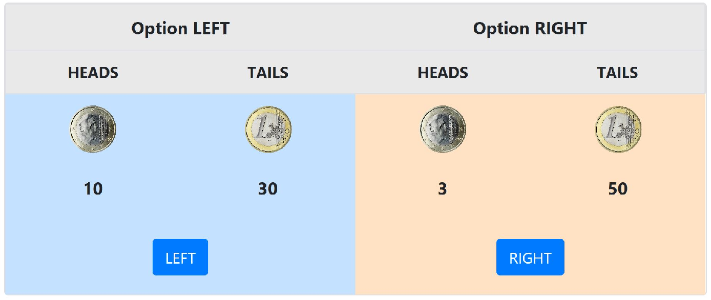
Your earnings from this part are determined as follows. At the end of the experiment, one out of the 20 decisions you made is randomly and with equal probability chosen for payment by the computer. Then, the respective lottery is simulated by the computer and you receive the outcome of the lottery converted to Euro according to the above exchange rate.
For example:
If the outcome is Heads, you will receive the Heads-amount of tokens converted to € of your chosen lottery (either left or right). If the outcome is Tails, you will receive the Tails-amount of tokens converted to € of your chosen lottery.
If you choose the lottery to the left in the example above, you will receive 10 Token (= € 2) if the outcome of the lottery is Heads; and you will receive 30 Token (= € 6) if the outcome of the lottery is Tails in case this lottery is relevant for payment. If you choose the lottery to the right in the example above, you will receive 2 Token (= € 0.60) if the outcome of the lottery is Heads, and you will receive 50 Token (= € 10) if the outcome of the lottery is Tails in case this lottery is relevant for payment.
Please note that there is no right or wrong answer. In each of the 20 decisions, please choose the lottery you prefer. Since all of the decisions have the same probability to be chosen for payment, it is optimal for you to pay equal attention to all decisions, since you do not know which of the 20 decisions is finally chosen for payment.
The compliance measures in Table 9 give an overview whether our participants followed the specific guidelines and exclusion criteria for our experiment. Participants were informed about those criteria already in the invitation for the experiment, and reminded when they received a reminder for the session a day before the actual experiment. Overall, we find a high rate of compliance with the self-reported measures in the questionnaire at the beginning of the experiment.
Table 9: Compliance Measures.
All Regular medication 4.64% Medical illness 3.09% Substance abuse 4.64% Smoke 6.7% Cups of coffee daily No coffee 52.06% 1 cup 28.35% 2 cups 11.86% 3 cups 5.67% 4 cups 1.55% 5 cups 0.52% Ability to abstain coffee for a day 94.85% Self-reported severe stress 15.46% Gum bleeding 0% Pregnancy or breastfeeding 0% Eaten within two hours prior to experiment 94.33% Brushed teeth prior to experiment 90.72% Woke up in time for experiment 98.97% Alcohol on day prior to experiment 93.30%
These criteria were important to ensure a reliable baseline measure of cortisol across participants, and to be able to measure cortisol in the saliva properly. Any substances such as medication, smoking, coffee, food in general, or alcohol can influence cortisol levels. Gum bleeding as well as not having brushed the teeth prior to the experiment can distort the cortisol measurement. Other factors such as severe stress, substance abuse, medical illness, pregnancy or breastfeeding as well as having eaten relatively close to the start of the experiment could also impact baseline levels of cortisol, but also cortisol reactivity in response to the stress treatment.
Whilst cortisol follows a diurnal rhythm, for example producing a peak after waking and declining throughout the day, a study by (Kudielka et al., 2004) finds that morning and evening sessions are comparable in their rates of cortisol activation in response to stress. A recent meta-analysis by (Goodman et al., 2017) also reports evidence that morning sessions of the TSST do not differ significantly in overall cortisol response from sessions at other times of the day. To address a potential differential effect of session time on cortisol reactivity in our sample, we conduct an exploratory analysis regressing the cortisol reactivity on the session time.
In addition, 28.24% of the female participants in our study reported to take the oral contraceptive (OC) pill. We include a test whether we also observe a differential impact of OC use on individual cortisol response in an exploratory analysis, in addition to a general effect on gender on cortisol reactivity. OC usage can attenuate the cortisol response: a recent meta-analysis by (Liu et al., 2017) finds significantly lower peak cortisol levels following the TSST for women using OC compared to both women not using OC and to men. As pre-registered, we exclude the gender category “other" from the from the analysis. In our sample, one subject chose this category.
Table 10 presents the results of OLS regressions with cortisol reactivity as the dependent variable. For this analysis, we had to exclude 9 subjects since their saliva samples were not sufficient to measure cortisol levels. we find a suggested significant effect of session time on cortisol reactivity (p < 0.05, column 1); OC-use does not have a significant impact (column 2).
Table 10: OLS regression results: Session time, OC use, and cortisol reactivity. This table shows the coefficients for the regression of treatment (Stress), session time, gender, and the interaction effect of gender and oral contraceptives on the cortisol reactivity, which is calculated as the difference in cortisol from baseline (Time 1) to the cortisol measurement after the stress or control task (Time 2). The variable session time takes on three values for sessions starting at 10am (session time = 1), 12pm (session time = 2), and 14pm (session time = 3). OC is a dummy indicating whether a subject identifying as female was taking OC or not. Robust standard errors are in parentheses. Stars indicate significance levels, * p < 0.05, ** p < 0.005; *** p < 0.001.
Cortisol reactivity (1) (2) Stress 0.719*** 0.721*** (0.076) (0.078) Session time 0.136* (0.052) Female 0.029 (0.091) OC x female –0.084 (0.109) Constant −0.572*** −0.303*** (0.111) (0.057) Observations 185 184 R-squared 0.349 0.323
Results of the exploratory analyses are presented in columns (2) and (3) of Table 10. Importantly, we note that the magnitude of the effect (and also the significance) of the treatment assignment variable on the cortisol reactivity does not change across the different specifications. We find that there is a suggested statistically significant effect of the session time of day on the cortisol reactivity, in a positive direction. The morning session was coded as 0, therefore this result indicates that there was a lower reactivity for the morning session relative to the mid-afternoon and late-afternoon sessions. There is no significant effect of gender or oral contraceptive use on the cortisol reactivity.
As pre-registered, since the number of safe choices as well as the number of reverse switches are ordered categorical outcome variables, we include Ordered Probit regressions as robustness checks in addition to the OLS regression as presented in the main analysis. We regress the treatment dummy, our measure for cognitive ability (overall score in the cognitive reflection task, where a maximum of four correct answers were possible), and an interaction effect of treatment and cognitive ability on the number of reverse switches.
Table 11 shows the results. The results confirm our findings of the main analysis, where cognitive abilities are negatively related to the number of reverse switches across both models, which is significant with p < 0.005 in the model only including the treatment dummy and CRT scores as explanatory variables (column 1), and suggested significant with p < 0.05 in the model also including the interaction effect between treatment and cognitive abilities as an explanatory variable (column 2).
Table 11: Ordered Probit regression results. This table shows the coefficients for the regression of treatment, a measure for cognitive abilities (CRT, which is the sum of all correct answers given in the cognitive reflection test with four questions), and the interaction of treatment and cognitive abilities on the number of reverse switches across both choice lists in risk task. Bootstrapped standard errors are in parentheses. Stars indicate significance levels, * p < 0.05, ** p < 0.005; *** p < 0.001.
Number of reverse switches (1) (2) Stress CRT Stress x CRT Observations 194 194 Pseudo R2
In this part, we provide two non-preregistered robustness checks. First, we present an analysis also including the session with the disruptive participant. Since this was an unplanned deviation from the pre-registration, we want to report these results to be as transparent as possible. However, we do not want to include this data in the main analysis since we did not send the saliva samples for that subset of subjects to be analyzed with respect to cortisol levels, so we do not have the full data. In addition, there could be many effects on observed behaviour that are unobserved and are also not clear in which direction they would go, and if that would be the same for the treatment and control group.
Second, we present an analysis for cortisol responders only. We think this is important since our fraction of actual subjects that had a significant increase in measured cortisol levels according to the saliva data was substantially smaller than what is observed in the literature on average: in our sample we had 52.69% cortisol responders, whereas in the literature the percentage of cortisol responders under stress is as high as 70-80%.
Table 12 presents summary statistics for the full dataset including the session with the disruptive participant. Overall, there are 206 observations with 106 participants in each treatment. The results are very similar to the results as reported in the main analysis: we do not find significant differences across conditions in CRT scores, which we see as an indication for successful randomization (p > 0.37). In addition, the negative affect score after the TSST is significantly higher for subjects in the Stress group compared to the no stress group with p < 0.001, whereas there is no significant difference in the beginning of the experiment (p > 0.55).
Table 12: Summary Statistics — Including Session with Disruptive Participant. Standard deviations are in parentheses. p-values are obtained using two-sided t-tests. The total number of possible safe choices was 20 (for all of the decisions in the two multiple price lists); the maximum number of reverse switches is therefore 10. Due to our four CRT questions, the maximum score in the CRT is 4. The possible maximum negative affect score is 50. N = 206
All No-stress Stress p-value Number of safe choices 12.98 12.84 13.12 0.57 (3.41) (3.32) (3.51) Number of reverse switches 1.74 1.90 1.58 0.25 (2.00) (2.09) (1.91) CRT score 2.27 2.19 2.35 0.37 (1.24) (1.26) (1.22) Negative affect score before TSST 15.63 15.41 15.84 0.55 (5.27) (4.94) (5.60) Negative affect score after TSST 18.84 15.88 21.80 0.00 (7.09) (5.30) (7.44)
We do not find any significant difference in the number of safe choices across treatments (p > 0.57), and also observed noise as measured by the number of reverse switches is not significantly different (p > 0.25).
Figure 7 illustrates the findings graphically, where we also add more information by adding the error bars representing the 95% confidence intervals.
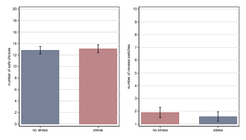
Figure 7: Mean number of safe choices across conditions [left]. This figure depicts the mean number of safe choices in the No-stress (red) compared to the Stress (blue) condition. The mean number of safe choices is calculated using both lists in the risk task. The error bars represent the 95% confidence intervals. Mean number of reverse switches across conditions [right]. This figure depicts the mean number of reverse switches in the No-stress (red) compared to the Stress (blue) condition. The mean number of switches is calculated using both lists in the risk task. The error bars represent the 95% confidence intervals.
Table 13 presents summary statistics for the subsample of participants who were defined as cortisol responders according to the prevalent measure in the literature, which is 52.69% of our full sample. Following the literature, we define an active cortisol response using a threshold of a 1.5nmol/L baseline-to-peak increase (Miller et al., 2013) (equivalently, a percentage increase of at least 15.5% for Time 2 compared to Time 1). A cortisol nonresponse is therefore an increase in cortisol less than this.
Table 13: Summary Statistics — Cortisol responders only. Standard deviations are in parentheses. p-values are obtained using two-sided t-tests. The total number of possible safe choices was 20 (for all of the decisions in the two multiple price lists); the maximum number of reverse switches is therefore 10. Due to our four CRT questions, the maximum score in the CRT is 4. The possible maximum negative affect score is 50.
All No-stress Stress p-value Number of safe choices 12.65 12.64 12.67 0.96 (3.36) (3.36) (3.41) Number of reverse switches 1.77 1.96 1.43 0.14 (2.04) (2.16) (1.76) CRT score 2.33 2.14 2.67 0.02 (1.24) (1.26) (1.14) Negative affect score before TSST 15.45 15.49 15.37 0.90 (5.23) (4.99) (5.70) Negative affect score after TSST 18.10 15.77 22.47 0.00 (6.88) (5.19) (7.57)
Overall, this leaves us with 141 observations, with 92 observations in the control group and 49 observations in the treatment group. Please note that for the cortisol analysis, for 9 subjects there was not a sufficient amount of saliva to analyze it with respect to cortisol levels, which means that there are also less than 97 observations in the control condition. The results are very similar to the results as reported in the main analysis: we find a suggested significant difference across conditions in CRT scores, which we see as an indication for successful randomization overall (p > 0.02). In addition, the negative affect score after the TSST is significantly higher for subjects in the Stress group compared to the no stress group with p < 0.001, whereas there is no significant difference in the beginning of the experiment (p > 0.90).
We do not find any significant difference in the number of safe choices across treatments (p > 0.96), and also observed noise as measured by the number of reverse switches is not significantly different (p > 0.14).
Figure 8 illustrates the findings graphically, where we also add more information by adding the error bars representing the 95% confidence intervals.
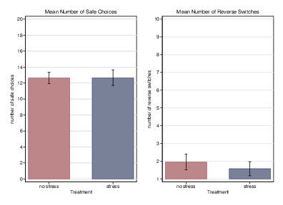
Figure 8: Mean number of safe choices across conditions [left]. This figure depicts the mean number of safe choices in the No-stress (red) compared to the Stress (blue) condition. The mean number of safe choices is calculated using both lists in the risk task. The error bars represent the 95% confidence intervals. Mean number of reverse switches across conditions [right]. This figure depicts the mean number of reverse switches in the No-stress (red) compared to the Stress (blue) condition. The mean number of switches is calculated using both lists in the risk task. The error bars represent the 95% confidence intervals.
Copyright: © 2022. The authors license this article under the terms of the Creative Commons Attribution 3.0 License.
This document was translated from LATEX by HEVEA.