Judgment and Decision Making, Vol. 17, No. 2, March 2022, pp. 234-262
Preference for playing order in games with and without replacement: Motivational biases and probability misestimations
Kwanho Suk*
Jieun Koo#
|
Abstract:
This research explores the preference for playing order in games in which
each of several players draws a random event (e.g., a ball from an urn), with and
without replacement after each draw. Three studies show that people tend to
prefer to draw early regardless of whether the game is with or without
replacement, although the expected probability of winning is the same
irrespective of the draw order. The reasons for preferring
earlier draws differ depending on the game type. For games without
replacement, the biased preference for earlier draws is related to
multiple motivational factors such as aversion to uncertainty, ambiguity,
and uncontrollability. Game valence also affects
draw order preference through the misestimation of winning probabilities:
people tend to prefer earlier draws in a gain-dominant game
(i.e., a higher probability of winning) but prefer later draws in a
loss-dominant game (i.e., a higher probability of losing). For games with
replacement, preference for earlier draws is mainly explained by
uncertainty aversion, with little bias in probability estimations.
Keywords: decision making, uncertainty aversion, ambiguity aversion, uncontrollability aversion, probability misestimation
1 Introduction
Suppose a simple game in which a player wins when she or he draws a red
ball from a box. The box contains 100 balls and six of them are red. A
hundred players take turns to draw a ball and then return the ball they
drew back to the box. Which turn would you want to take in playing the
game? This type of game is called a game with replacement. The winning
odds of such a game do not vary with playing order because the preceding
outcomes (e.g., your friend won the prize) do not affect the probabilities
of later draws.
Another type of a game is a game without replacement. In the same game, one
does not return the ball into the box after a draw. Then, previous results
change the winning chance of later draws (e.g., your friend’s winning of
the prize means that you have a reduced chance). This is typical of a game
without replacement. Let us consider another example. Suppose that an
electronic shop launches a mystery box promotion. The mystery box includes
Apple’s products and 100 eligible customers can buy one. The customers do
not know what products are inside the box until they purchase and open
one. The shop announced that six out of the 100 mystery boxes include a
brand-new MacBook that you desire badly. Luckily, you were one of the 100
persons. On the mystery box promotion day, the 100 people wait in line,
with most of them dreaming of winning a jackpot. The purchase order is
according to the position of the waiting line. The shop sells boxes in
completely random order. This mystery box promotion is an example of a
game without replacement if the boxes purchased by consumers are not
replaced with the same ones.
Suppose that the purchase has not started yet. Then, which turn do you
prefer? First, second, third, middle, or last? Do you think that the
probability of winning a MacBook changes with your purchase order? Now,
the purchase has started and 90 people have bought a mystery box. You are
one of the last ten people in line. Surprisingly, none of the 90 people
got a MacBook. Therefore, out of the ten remaining boxes, six include a
brand-new MacBook. This circumstance still falls under a game without
replacement, with a change in winning odds from 6% to 60%. Then when do
you want to purchase? Right now, or wait for longer? Does the order matter
in winning a MacBook now?
The answer is that in any case, the purchase order does not matter. In
games without replacement, previous outcomes change the winning
probabilities of later draws, such as from 6% to 60% in the mystery box
case. Given the changed probability, however, the draw order does not
alter the winning probabilities. Nevertheless, a simple pre-test
(N = 95) showed that more than 60% of the respondents answered
that the chance of winning differs depending on the game order for games
without replacement.
In summary, a rational decision maker should be indifferent to the draw
order in both games with and without replacement if the chance of winning
is the only consideration. The current research, however, suggests that
people have biased preference for playing order. We posit that
motivational factors and probability misestimation affect preference for
draw orders and that their influences vary depending on the game type. For
games with replacement, motivational factors such as uncertainty aversion
make people prefer earlier orders. However, probability misestimation
should have a weak or no influence because of the game’s simple structure.
For games without replacement, both motivational and probability
(mis)estimation would affect draw order preference because every draw
keeps changing the winning probability. People prefer to take earlier than
later draws because of motivational factors such as uncertainty aversion,
ambiguity aversion, and uncontrollability aversion, and this tendency is
moderated by game valence as a result of probability misestimation.
Specifically, compared with a neutral game (50–50 chance), an earlier draw
is preferred in a gain-dominant game (high probability of winning),
whereas a later draw is preferred in a loss-dominant game (high
probability of losing).
From a theoretical perspective, this study investigates preference for game
order, a feature that has been received little attention in
decision-making research. Previous studies have mostly focused on one-shot
binary-choices with fixed probabilities of winning (e.g., choices between
two options with different probabilities and amounts of gains). This work
examines games with multiple players and explores the mechanism whereby
people choose the playing order. In particular, studying a game without
replacement provides insights about decision making processes when dynamic
changes occur in the probability of winning.
This paper is organized as follows. First, we demonstrate that winning
probabilities are unaffected by the playing order in games with and
without replacement. We then propose motivational factors and probability
misestimation as the main forces that drive playing order preferences.
Studies 1 and 2 test games without replacement and report empirical
evidence for biases in playing order preference. Study 3 tests a game with
replacement. Lastly, we discuss the theoretical and practical implications
of the current research.
1.1 Game order and probability of winning
Games with replacement are simple to understand because the preceding
outcome does not change the winning probability of later draws. Thus, it
is straightforward that all draws have the same chance of winning. People
with very basic knowledge of probability are aware of this fact.
Therefore, a rational decision maker should not show preference for some
specific draw orders if the chance of winning is the only concern.
By contrast, games without replacement are complex because the winning
probability changes every time a draw is made as the game moves onward.
However, the winning probability is unaffected by the draw order, although
prior outcomes affect the winning likelihoods themselves. The following
example illustrates that the expected probability of winning is not
affected by the draw order in a game without replacement. In a game,
players draw balls from an urn containing n balls, with x
red balls and n−x white balls. A player who draws a red ball
wins the game (outcome: W), whereas one who draws a white ball loses the
game (outcome: L). Balls are drawn from the urn one at a time, and the
drawn balls are not replaced. Players decide the order in which they draw.
In this game, the expected probability of winning at the i-th turn,
p(Wi), follows a hypergeometric distribution and has two important
properties. First, if the result of the draw is unknown (e.g., before the
draw), every draw in the sequence has the same probability of winning,
p(Wi) = x/n = p. In the first draw, the probability of winning is simply
p(W1) = p. In the second and later draws, the calculation is more
complicated and involves joint and conditional probabilities. In the second
draw, the expected probability of winning is the sum of the conditional
winning probabilities in that draw given the result of the first draw, as
shown in Equation (1). The expected winning probability of the second draw
is also p(W2) = p. Similarly, the expected probabilities of winning in
the third and later draws are the same as p but require a more
complicated computation.
p(W_2)=p(W_1∩W_2)+p(L_1∩W_2)
=p(W_1) ·p(W_2|W_1)+p(L_1) ·p(W_2|L_1)
=x/n ·x-1/n-1+n-x/n ·x/n-1
=x/n=p
Second, once the game starts, the results of earlier draws change the
expected probability of winning at the i-th turn, p*(Wi). Given this
altered probability, however, the draw order does not affect the winning
probabilities for later draws. That is, the game resets to a game with the
altered probability of winning that is determined by the remaining
balls. For example, the probability of winning in the second draw,
p*(W2), is determined by the first draw result. With the remaining
balls, the game resets to the changed probability, and the expected
probability of winning for later draws is the same as p*(W2).
Figure 1 presents a specific example of the game results and probabilities.
Five players participate in a game of drawing a ball from an urn containing
three red (winning) balls and two white (losing) balls. The expected
probability of winning in the i-th draw, p(Wi), is always .60,
regardless of the draw order. For the first player, the expected
probability of winning, p(W1), is merely .60. For the second player, the
probability of winning, p(W2), is the same as that of the first player
despite being dependent on the first draw result. When the first player
wins by drawing a red ball (probability of .60), the urn then contains two
red balls and two white balls. Given the first result, the conditional
probability of winning for the second drawer is .50. The probability that
the second player would win in this case is
p(W1 ∩ W2) = .60 · .50 = .30. However, if the first player
draws a white ball (probability of .40), three red balls and a white ball
would remain in the urn. In this case, the second player’s conditional
probability of winning is .75. The probability that this outcome would
occur is p(L1 ∩ W2) = .40 · .75 = .30. Thus, the expected
probability of the second player’s winning is expressed as
p(W2) = p(W1 ∩ W2) + p(L1 ∩ W2) = .60, which is equal to
the first player’s winning probability.
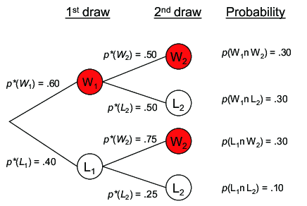
| Figure 1: Outcomes and their probabilities for a hypothetical game
without replacement. This figure shows the possible outcomes and their
probabilities in the first two draws of a no-replacement game with three
red (winning) balls and two white (losing) balls. |
Once the game starts and the outcome of the first draw is known, the
probabilities of winning for later draws change. In the example, if the
result of the first draw is a win, the probabilities of winning in the
later draws would change from .60 to .50. Given the changed winning odds,
the game resets as one with two winning balls and two losing balls.
Moreover, the expected winning probabilities for all remaining draws are
the same as .50 until the draw of the next ball. Therefore, a rational
decision maker should be indifferent to the draw order in a game without
replacement because the order does not affect the chances of winning.
Taken together, the draw order does not matter for games with and without
replacement. However, theories on decision making suggest that players
prefer to draw early in the games and this tendency is moderated by game
valence, especially for no-replacement games.
1.2 Psychological
factors affecting playing order
1.2.1 Motivational factors
In games with and without replacement, some motivational factors should
favor earlier rather than later draws. These factors include the
tendencies of people to avoid uncertainty, ambiguity, and
uncontrollability. Uncertainty aversion affects both games with and
without replacement. However, ambiguity and uncontrollability aversion
influence only the games without replacement.
Uncertainty aversion. People have a tendency to disfavor
uncertainty when outcomes are probabilistic. People feel anxious in
uncertain situations, and this anxiety motivates them to resolve the
uncertainty as soon as possible. Uncertainty aversion is a robust
phenomenon that characterizes decision making in gambling, investments,
and consumer choice (Gneezy et al., 2006; Kahneman & Tversky, 1979;
Newman & Mochon, 2012; Simonsohn, 2009). The principle also predicts that
for games with and without replacement, people are likely to resolve
uncertainty by taking an early draw because it frees them from anxiety and
also gratifies curiosity about the result (Calvo & Castillo, 2001;
Loewenstein, 1994; Lovallo & Kahneman, 2000). Therefore, we expect that
regardless of replacement, the need to resolve uncertainty drives
preference for drawing early, rather than late.
Ambiguity aversion. Individuals prefer situations wherein the
apparent “objective” probabilities of outcomes are known with certitude,
rather than are unknown or uncertain (Camerer & Weber, 1992; Güney &
Newell, 2015). Disliking this lack of information is called ambiguity
aversion. In Ellsberg’s (1961) well-known example, an urn contains 90 red,
black, and yellow balls. Of the 90 balls, 30 balls are red. The other 60
balls are either black or yellow but the exact number of each color is
unknown. Participants bet on the color of the ball drawn from the urn. In
this case, people tend to select red, although the other colors have the
same odds of winning. This example shows a tendency to prefer known
chances (e.g., red balls) to the unknown (e.g., black or yellow
balls).
The tendency to avoid an “unknown probability” should motivate an early draw
in a no-replacement game. The available proportions of later winning
draws are not clearly known in advance because they can be altered
according to the results of earlier draws. In the first or earlier draw,
however, the chance of winning is rather clearly known. Therefore,
ambiguity aversion is expected to lead to preference for early draws. By
contrast, the winning chances of games with replacement are fixed,
and therefore ambiguity aversion should have little effect.
Uncontrollability aversion. The desire for control also predicts
preference for an early draw in no-replacement games. People have a desire
for control and tend to avoid uncontrollable situations (Cutright, 2012;
Cutright & Samper, 2014; Langer, 1975). For example, people are happier
when they believe outcomes are due to their own decisions and actions
rather than due to external forces (Shojaee & French, 2014). In a
no-replacement game, an early draw’s outcome is determined by the player’s
own action, but the results of later draws are determined by the previous
draws. Therefore, the desire for control should lead to preference for
early draws. In a game with replacement in which others’ decisions do not
have any influence, uncontrollability aversion should have little effect
on order preference.
1.2.2 Probability misestimation
Another factor affecting playing order preference is probability
misestimation, one that we expect to have a significant effect only for
no-replacement games. We posit that the extent to which one prefers early
draws is moderated by the winning probability of a game. Suppose that
three no-replacement games with different odds of winning are carried out.
In the first game, 75% of the balls are of a winning color and 25% are
of a losing color (i.e., a gain-dominant game). In the second game, 25%
of the balls are of a winning color and 75% are of a losing color (i.e.,
a loss-dominant game). The third game has an equal number (50%) of
winning and losing balls (i.e., a neutral game). The inclination to prefer
an early draw is expected to be greater in a gain game than in a loss
game. We conjecture that this effect occurs because of the erroneous
estimates of the winning probability as people tend to rely on judgment
heuristics rather than on computations of relative frequencies
(Gilovich et al., 2002; Kahneman et al., 1982).
Judgment heuristics related to probability misestimation in a
no-replacement game arise from ignorance of conditional probabilities and
the representativeness heuristic (Kahneman & Tversky, 1972; Tversky &
Kahneman, 1981). The winning probability in the first draw is rather
simple. However, probability estimation for later draws requires a more
complicated calculation involving conditional probabilities and joint
probabilities, and thus individuals tend to ignore conditional probability
(Tversky & Kahneman, 1981). This ignorance results in a greater chance of
probability misestimation (Bar-Hillel, 1973; Gneezy, 1996; Tentori et al.,
2013).
Furthermore, the representativeness heuristic systemically biases the
direction of misestimation. According to the representativeness heuristic,
the likelihood of a specific event is overestimated when it resembles the
salient features of the population (Bordalo et al., 2016; Kahneman &
Tversky, 1972). If players rely on the representativeness heuristic in a
no-replacement game, then they would estimate the likelihood of a winning
or losing outcome based on the similarity with the population’s salient
features. Consider a game with six winning balls and two losing balls.
When guessing for earlier turns, the representativeness heuristic suggests
that one would overestimate the likelihood of a winning ball because the
population includes more winning balls which constitute a salient feature.
This bias naturally leads to the belief that for later draws, the less
salient feature (i.e., a losing ball) is more likely to be drawn. This
pattern in a no-replacement game does not necessarily imply the gambler’s
fallacy, which explains the perceived negative autocorrelation in games
with replacement with constant probabilities.
In short, ignorance of conditional probabilities and the representativeness
heuristic imply that the subjective probability for an early (late) draw
is biased toward the event with the higher (lower) objective probability
of occurrence. Thus, when gains are salient, individuals estimate the
chance of winning as higher for earlier draws and lower for later draws.
On the other hand, when losses are more salient, the estimation of the
winning probability would decrease for earlier draws but increase for
later draws. In a neutral frame game with a 50–50 chance of winning and
losing, neither gains nor losses are more salient. Therefore, the
misestimation of the probabilities is less likely compared with the gain
or loss games.
2 Study 1: A game without replacement
Study 1 aims to show the draw order preference in a game without
replacement and the moderating role of game valence. Participants were
asked to indicate their preferred draw order under a scenario that varies
in the game’s valence and size.
2.1 Method
A total of 168 university students (34.3% females,
Mage = 21.9) participated in a 3 (game valence:
gain vs. loss vs. neutral) x 2 (game size: 8 vs. 24) between-subjects.
Participants were presented with a hypothetical game scenario. They were
asked to imagine themselves playing the game with other people. In the
game, each person draws a ball from an urn containing red and white balls.
The drawn balls are not replaced. The player who picks a red ball wins
$10 and the one who picks a white ball loses $10.
The valence of game was manipulated by the ratio of red and white balls. In
the gain condition, the game offered a 75% chance of winning and a 25%
chance of losing (p(W) = .75). In the loss condition, these
probabilities were reversed, with a 75% chance of losing and a 25%
chance of winning (p(W) = .25). In the neutral condition, the
odds were 50:50 (p(W) = .50). The game size was also manipulated.
The scenario described either a game with eight participants drawing balls
from an urn containing eight balls (small size) or a game with 24
participants with 24 balls (large size). Because the game size is added
for testing generalizability1, the main test compares the three
valence conditions. Our sample size is close to a minimum of 64
participants in each valence group for having a statistical power of .80,
given the assumption of moderate effect size (Cohen’s d = .50)
because no similar previous studies exist.
Participants indicated their preferred draw order through an open-ended
question and then wrote down the reasons for their preference. We also
measured the estimates of the winning probability if they drew first,
middle (4th in the 8-person game and 12th in the 24-person game), and last
on a 101-point sliding-bar scale ranging from 0% to 100%.
2.2 Results
Preference for draw Order. First, the draw order preferences in
the large game (range of 1 to 24) were converted to a range between 1 and
8. Specifically, a preference for 1st, 2nd, or 3rd draw in the large game
was defined as a 1st draw preference, a preference for a 4th, 5th, or 6th
draw as a 2nd draw preference, and so forth.2
The distribution of preferences showed that most participants favored early
draws (Figure 2). Overall, 51.2% preferred to draw first, and 83.3%
preferred to draw first, second, or third. In all six conditions, the
average preferred draw order was significantly lower than the median of
4.5 (t > 5.59, p < .001, Cohen’s
d > 1.08). Table 1 presents the average of the
preferred order in each condition. These results provide strong evidence
that people prefer early draws in games without replacement.
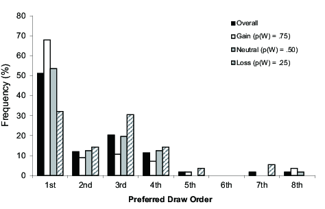
| Figure 2: Distributions of draw order preference in Study 1. |
| Table 1: Preferred draw order as a function of game valence and
size in Study 1. |
| | Gain | Neutral | Loss |
| | (p(W) = .75) | (p(W) = .50) | (p(W) = .25) |
| Small Game | 1.96 | 2.11 | 2.78 |
| Large Game | 1.71 | 1.93 | 2.52 |
| | [3.64] | [4.64] | [6.24] |
| Note. The preferred order in the large game condition was
transformed so that the value ranged between 1 and 8. The raw preferred
orders in the large game condition (1 to 24) are in brackets. |
Game valence. Table 1 also shows that the draw order preferences
were influenced by how the game was valanced. A 3 (game valence: gain vs.
neutral vs. order) x 2 (game size: 8 vs. 24) ANOVA on the preferred draw
order revealed that only the main effect of valence was significant
(Mgain = 1.84 vs.
Mneutral = 2.02 vs.
Mloss = 2.65); F(2, 162) = 4.31,
p = .015, ηp2 = 0.05). Neither the main effect of game
size (M8 = 2.28 vs. M24
= 2.05; F(1, 162) = 0.95, p = .332, ηp2 = 0.01)
nor the interaction (F(2, 162) = 0.01, p = .988,
ηp2 < 0.01) was significant. In the analyses reported
below, the small and large size conditions were combined because the effect
of game size was not significant.
The follow-up marginal mean comparisons indicated that participants
preferred earlier draws for the gain game than for the loss game
(Mgain = 1.84 vs.
Mloss = 2.65; F(1, 162) = 7.85,
p = .006, d = 0.53). The preferred order with the neutral
game (M = 2.02) fell between the gain and loss games and was
significantly earlier than the loss game (F(1, 162) = 4.75,
p = .031, d = 0.41) but was not significantly different
from the gain game (F(1, 162) = 0.39, p = .534,
d = 0.12).
Similarly, the percentage of participants preferring to draw first differed
as a function of valence (Figure 2). The percentages of participants who
preferred to draw first were 68% in the gain game, 54% in the neutral
game, and 32% in the loss game (χ2(2,
N=168) = 14.48, p = .001, φ = 0.29).
Reasons for order preference. We also analyzed
participants’ stated reasons for their draw order preferences. Two trained
judges conducted content analysis of these reasons. On the basis of the
hypothesis of this study, the judges classified the stated reasons into
(1) uncertainty aversion, (2) ambiguity aversion, (3) uncontrollability
aversion, (4) probability (mis)estimation, and (5) others. The statement
of a participant could include more than one type of reason. Disagreements
were resolved by discussion.
Statements revealing discomfort about the uncertainty of the game (e.g., “I
want to know the result as early as possible because I am too nervous to
wait.”) were classified as uncertainty aversion statements. Those
statements that expressed concern about not being able to determine the
exact odds of winning on later draws were classified as ambiguity
aversion. Uncontrollability aversion statements expressed concern about
the results possibly being determined by others, instead of by the player
herself or himself. Statements regarding probabilities were further
divided into four categories: (i) early draws have a higher probability of
winning, (ii) middle draws have a higher probability of winning, (iii)
later draws have a higher probability of winning, and (iv) draw order is
unrelated to the probability of winning. The first three categories were
considered misperceptions regarding the probability of winning.
First, a multiple regression analysis3 was employed to test whether the reasons are related to
the preferred draw order in all the valence conditions
combined. Specifically, the preferred draw order was regressed on the cited
reasons for preference. The estimated standardized beta coefficients are
presented in Column 2 of Table 2. Motivational factors were related to the
preference for early draws, as indicated by the significant negative beta
coefficients for uncertainty aversion (β = –.30, t(160) =
4.36, p < .001), ambiguity aversion (β
= –.20, t(160) = 2.97, p = .003), and uncontrollability
aversion (β = –.15, t(160) = 2.30, p =
.023). Tests about probability estimation showed that mentioning an
early-draw advantage was significantly related to preference for earlier
draws (β = –.36, t(160) = 4.80, p
< .001), whereas mentioning a late-draw advantage was
significantly related to preference for later draws (β
=.29, t(160) = 4.45, p < .001). However,
statements that expressed an advantage for a middle draw (β
= .05, t(160) = 0.68, p = .500) or statements that
mentioned no relation between draw order and probability (β
= –.14, t(160) = 1.81, p = .073) were not significantly
related to draw order preference.
| Table 2: Stated reasons for preferred draw order as a function of
game valence in Study 1. |
| | | Percentage (frequency) of participants who mentioned the reason for preference |
| | Regression β | Total | Gain | Neutral | Loss |
| Motivational Factors | | | | | |
| Uncertainty aversion | β = –.30** | 14% (23) | 16% (9) | 13% (7) | 13% (7) |
| Ambiguity aversion | β = –.20** | 8% (13) | 5% (3) | 11% (6) | 7% (4) |
| Uncontrollability aversion | β = –.15** | 21% (35) | 14% (8) | 29% (16) | 20% (11) |
| Probability Estimation | | | | | |
| Early draw advantage | β = –.36** | 24% (40) | 36% (20) | 18% (10) | 18% (10) |
| Middle draw advantage | β = .05 | 19% (31) | 14% (8) | 7% (4) | 34% (19) |
| Late draw advantage | β = .29** | 1% (2) | 0% (0) | 0% (0) | 4% (2) |
| Order is not related | β = –.14* | 24% (41) | 20% (11) | 34% (19) | 20% (11) |
| Note. Regression betas are standardized beta coefficients from a
multiple regression analysis that tests the relationship between each type
of reason and preferred order. The number of participants is in parentheses. * p < .10,
**p < .05. |
Second, chi-square tests examined whether the stated reasons differed
across the game valence conditions. Note that “ambiguity aversion” and
“late draw advantage” were excluded from the test because they failed to
satisfy the assumptions for chi-square tests (e.g., minimum 5 expected
observations per cell). Table 2 (Columns 4 to 6) presents the percentage
and frequency of
participants who stated each type of reason in each valence
condition. Mentioning motivational forces (aversions to uncertainty and
uncontrollability) related to a preference for early draws did not differ
as a function of valence, as indicated by the insignificant chi-square
tests (ps > .171). However, the percentages of
participants who indicated that “early draws have a higher probability of
winning” (χ2(2, N=168) = 6.56, p = .038, φ =
0.20) and “middle draws have a higher probability of winning” (χ2(2,
N=168) = 14.32, p = .001, φ = 0.29) differed as a
function of game valence. Follow-up tests revealed that the percentage of
participants whose statements favored early draws was significantly higher
in the gain game (36%) than in the neutral game (18%; z = 2.13,
p = .033, h = 0.41) and in the loss game (18%; z = 2.13)
p = .033, h = 0.41. On the contrary, the advantage of middle draws
was mentioned more frequently in the loss game (34%) than in the gain game
(14%; z = 2.43, p = .015, h = 0.48) and the neutral game
(7%; z = 3.51, p < .001, h = 0.71).
Winning odds estimation. We also tested whether the estimates of
the winning probability for the first, middle, and last draws were
influenced by game valence (Figure 3). The results of a 3 (game valence:
gain vs. neutral vs. loss) x 3 (draw order: first vs. middle vs. last)
mixed ANOVA showed a significant main effect of game valence F(2,
165) = 164.51, p < .001, ηp2 = 0.67), a
significant main effect of draw order (F(2, 330) = 58.64,
p < .001, ηp2 = 0.26), and a significant two-way
interaction (F(4, 330) = 5.98, p < .001,
ηp2 = 0.07). The significant main effect of game valence was expected
because the odds of winning were manipulated to be different across the
game valence conditions (Mgain = .63 vs.
Mneutral = .47 vs. Mloss
= .26). The significant main effect of the draw order indicates that
participants believed that the winning probabilities were higher for the
earlier draws (Mfirst = .50 vs.
Mmiddle = .48 vs. Mlast
= .37).
The significant interaction indicates that the influence of draw order on
estimated probability differed as a function of game valence. Cell-mean
contrasts were conducted for each valence condition. For the gain game, the
estimated probabilities of winning were highest in the first draw, second
highest in the middle draw, and lowest in the last draw
(Mfirst = .72 vs.
Mmiddle = .62 vs. Mlast
= .55). All these estimated probabilities significantly differed from one
another (F(1, 330) > 9.54, p <
.002, d > 0.58). For the loss game, the estimated
probabilities of winning were highest in the middle draw, second highest in
the first draw, and lowest in the last draw
(Mfirst = .27 vs.
Mmiddle = .31 vs. Mlast
= .19). Again, all the differences were significant
(F(1, 330) > 4.47, p < .035,
d > 0.40). For the neutral game, the estimated
probabilities in the first and middle draws were the highest. They did not
differ significantly from each other (Mfirst = .52
vs. Mmiddle = .50; F(1, 330) = 0.90,
p = .343, d = 0.18) but were significantly higher than the
last draw (Mlast = .38; F(1, 330)
> 31.95, p < .001, d
> 1.07). Figure 3 shows the estimated probabilities in each
condition.
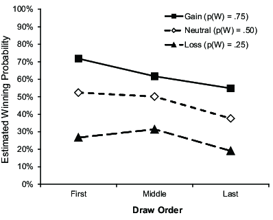
| Figure 3: Estimated probabilities of winning with the first,
middle, and last draws in Study 1 |
2.3 Discussion
The results of Study 1 provide evidence that individuals prefer early draws
in a game without replacement. This preference can be explained by
motivational factors such as the avoidance of uncertainty, ambiguity, and
uncontrollability. In addition, game valence affects draw order
preferences. When winning is more salient, participants prefer an early
draw. Conversely, participants opt for a later draw when the loss is more
prominent. This influence of game valence on draw order is related to the
misestimation of winning probability. Specifically, participants tend to
believe that the winning probability is higher for early draws than for
later draws when the winning odds are high. However, participants tend to
believe that middle draws have the highest probability of winning when the
odds of losing are high.
A noteworthy finding of Study 1 is that the estimated probability of
winning was lowest in the last draw, regardless of game valence (Figure
3). Although unexpected, this finding can be explained by vividness and
uncontrollability. First, imagining what will happen (i.e., vividness) is
more difficult for very late draws. People tend to underestimate the
likelihood of events that are difficult to imagine (Gregory et al., 1982;
Sherman et al., 1985). Thus, low vividness for late draws leads to an
underestimation of winning probabilities. Second, people tend to
underestimate probabilities when they have no control over the outcome,
whereas they overestimate the likelihood of success when the source of
uncertainty is internal (Brown & Bane, 1975; Howell, 1971). This finding
implies that participants underestimated the odds for later draws because
they perceived themselves as having less control in later draws than in
earlier draws.
In summary, Study 1 demonstrates a preference for drawing order and tests
the factors that influence this preference in a hypothetical game.
However, it is uncertain whether the same findings would be observed in a
real game with actual players and real monetary incentives. Thus, Study 2
tests preferences for draw orders in a real game situation.
3 Study
2: A game without replacement with monetary outcomes
In Study 2, groups of six participants played a real game without
replacement. Players drew a ball from a bag one by one, and those who drew
a ball of a winning color received a $3 prize, whereas those who drew a
ball of a losing color lost $3. The dependent variable was the
participants’ decisions regarding whether to draw right away or defer
their draw. Although the results of preceding draws determine the winning
probability for a given draw, the same probability applies to all later
draws including the given draw. We tested whether the “draw-or-defer”
decision is influenced by the probability of winning (i.e., game valence)
at each turn.
3.1 Method
A total of 84 university students (32.1% females,
Mage = 21.3) participated on a voluntary basis.
Participants were informed that they would receive $6 as game money and
play a game twice, betting $3 on each gamble. They were divided into 14
groups of six persons. Participants who knew one another well were
assigned to different groups to avoid potential social influence.
Before the game, the experimenter explained the procedure of the game in
detail. Participants would draw a ball out of a pouch containing three
orange and three white ping-pong balls. A participant who draws an orange
ball would receive $3, whereas one who draws a white ball would lose $3.
The priority to decide whether to draw or defer was randomly determined by
having participants pick a card with a number from 1 to 6. The person with
the lower number had priority in deciding whether he or she would draw or
defer at each turn. At each draw, the participant with the top priority
(with the lowest number) was asked to decide whether he or she would draw
at this turn. Once a participant drew a ball, he or she no longer had a
chance to draw again for the game. Everyone else could see the outcome and
the experimenter told them the number of remaining winning and losing
balls. If the participant decided to defer, then the one with the next
priority would decide whether or not to draw. If everyone decided to
defer, the one with the lowest priority had to draw a ball (This case was
excluded from the analyses because the draw was forced). The game
continued until all six people in a group drew a ball. However, when the
remaining balls were of the same color (e.g., three orange balls remain in
the pouch after a streak of a white ball for the first three draws) or
only one ball remained, the gamble turned into a certain game without
uncertainty. Then, these game outcomes were determined without
participants’ draw or defer decisions. After the game, the winners
received $3, whereas the losers paid $3 to the experimenter.
The same game was played twice. The procedure of the second game was the
same, except that the priority to make a decision was randomly determined
again for the second game. During the game, the experimenter recorded the
draw-or-defer decisions and the results of the draws. A total of 172
draw-or-defer decisions (79 decisions in game 1 and 93 decisions in game
2) were made by the players. Note that the dependent variable we analyzed
was the decisions rather than the players. For example, if the first two
players deferred their decisions and the third players drew a ball, then
they were counted as two defer decisions and one draw decision. When a
game outcome was decided without a player’s decision (e.g., only one ball
remaining), it was not counted as a player’s draw-or-defer decision.
3.2 Results
We tested the influence of the winning probability at each turn on the
draw-or-defer decisions. Due to the nature of the game, the odds of
winning changed as the game progressed, depending on which ball was drawn
in the preceding draws. For example, if the first ball was orange, then
the pouch would contain two orange balls and three white balls, thereby
resulting in a 40% probability of winning. For each draw, the winning
probability was calculated and the influence of this probability on the
draw-or-defer decision was tested. If the outcome was determined without
the player’s decision (e.g., one ball remains or the remaining balls are
of the same color) or a draw decision was forced, then we excluded those
draws from the analysis.
Before testing the hypotheses, the differences between the two games were
tested. No significant differences were found between the two games in the
draw-or-defer decisions (χ2(1, N=172) = 0.37, p =
.374, φ = 0.04). Thus, the games were collapsed4, thereby resulting in
28 games.
Table 3 presents the percentages of the draw and defer decisions for each
turn. Participants chose to draw more frequently than defer, and the
probability of winning moderated this decision. In the first draw,
participants were more likely to draw (76%) rather than to defer (24%).
A goodness-of-fit test shows that the decisions deviated significantly from
randomness, thereby indicating a preference for drawing to deferring
(χ2(1, N=37) = 9.76, p = .002, φ = 0.51). In
the second, third, and fourth draws, the winning probability strongly
influenced the decision. In the second draw, the winning probability was
.60 when the first draw was a loss and .40 when the first draw was a
win. When the winning probability was .60, 79% chose to draw, compared
with 46% when the winning probability was .40, and the difference was
significant (χ2(1, N=45) = 4.92, p = .027, φ
= 0.33). Similarly, in the third draw, the percentages of participants who
chose to draw were 100%, 79%, and 45%, when the winning odds were .75,
.50, and .25, respectively (χ2(2, N=38) = 7.65, p =
.022, φ = 0.45). In the fourth draw, 100% of participants chose to
draw when the winning probability was .67, whereas the draw rate was 53%
when the winning probability was .33 (χ2(1, N=33) = 9.12,
p = .003, φ = 0.53). In the fifth draw, 95% decided to draw
when the winning probability was 50% (one orange ball and one white ball
remaining), thereby indicating a strong preference for drawing to deferral
(χ2(1, N=19) = 15.21, p < .001, φ =
0.89). Figure 4 graphically illustrates the participants’ decisions in the
first, second, and third draw turns given the results of the preceding
draws.
| Table 3: Draw or defer decisions as a function of the probability
of winning in Study 2. |
| | 21.5in
Probability of winning
(orange/white balls) | Decision | |
|
Draw turn | | Draw | Defer | χ2 test |
| 1 | 50% (3/3) | 76% | 24% | χ2(1, N=37) = 9.76* |
| | | (28) | (9) | |
| 2 | 40% (2/3) | 46% | 54% | χ2(1, N=45) = 4.92* |
| | | (12) | (14) | |
| | 60% (3/2) | 79% | 21% | |
| | | (15) | (4) | |
| 3 | 25% (1/3) | 45% | 55% | χ2(2, N=38) = 7.65* |
| | | (5) | (6) | |
| | 50% (2/2) | 79% | 21% | |
| | | (15) | (4) | |
| | 75% (3/1) | 100% | 0% | |
| | | (8) | (0) | |
| 4 | 33% (1/2) | 53% | 47% | χ2(1, N=33) = 9.12* |
| | | (10) | (9) | |
| | 67% (2/1) | 100% | 0% | |
| | | (14) | (0) | |
| 5 | 50% (1/1) | 95% | 5% | χ2(1, N=19) = 15.21* |
| | | (18) | (1) | |
| Note. Chi-square tests in the first and fifth draws tested
goodness-of-fit assuming a 50% draw-defer split. Chi-square tests in the
second, third, and fourth draws examined whether a draw-or-defer decision
was associated with the winning probability. The number of each decision
is in parentheses. *p < .05. |
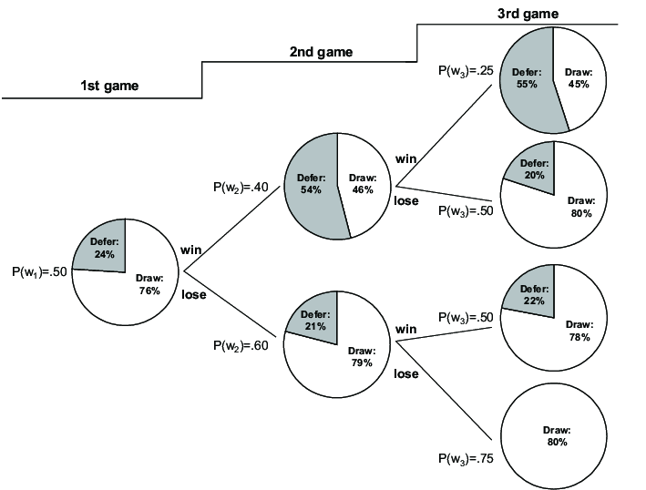
| Figure 4: Draw-or-defer decisions for the first, second, and third
turns in Study 2. The pie charts show the percentages of participants who
decided to draw and defer with odds of winning
p*(wi). These odds were
determined by how many winning and losing balls remained in the pouch
after the preceding draw was made. |
In addition, the potential influence of various factors on the
draw-or-defer decision was tested. First, the draw-or-defer decisions were
not influenced by the decision of the person in the immediately preceding
turn (χ2(1, N=142) = 3.00, p = .083, φ =
0.15).5 Second,
no significant influence of decision priority was found on the
draw-or-defer decisions (χ2(4, N=172) = 3.91, p =
.419, φ = 0.15). Third, the outcome of the first game (winning or
losing $3) had no significant effect on the draw-or-defer decisions in the
second game (χ2(1, N=93) = 0.15, p = .701),
φ = 0.04.)
3.3 Discussion
Study 2 replicated the findings of Study 1 in a different setting. First,
real monetary incentives were provided. Second, participants had real
competitors and made actual decisions given the outcomes of earlier draws.
Thus, the same findings were obtained for a situation wherein decision
making is more consequential and complicated.
We have explored decision making in games without replacement. In the next
study, we change a game type, from without replacement to with
replacement. This aims to test whether preference for playing order
differs depending on with or without replacement.
4 Study 3: A game with replacement
Unlike our previous studies, Study 3 tests preference for play order in the
game of rolling dice, a typical game with replacement. Participants were
asked to imagine that six people including themselves would roll the dice
once and that winning or losing some money depends on the number they get.
This game with replacement is simple and easy for estimating the winning
chance because the previous results do not affect the later one (i.e., the
dice have no memory). Given the transparency of the game, we expect that
ambiguity aversion, uncontrollability aversion, and probability
misestimation hardly cause biases. However, uncertainty aversion would
remain because the outcomes of dice rolling are still probabilistic.
Consequently, participants in the dice game would still favor early rolls
as in games without replacements. Furthermore, this tendency would not be
moderated by game valence in contrast to games without replacement because
probability misestimation is less likely to occur.
4.1 Method
A total of 105 university students (48.6% females,
Mage = 22.4) participated in a one-way
between-subjects design study that manipulated game valence (gain vs. loss
vs. neutral). The sample size meets a minimum of 17 participants per cell
for a power of .80, according to the effect size about playing order of
Study 1 (Cohen’s d = 1.0). Participants were asked to imagine that
six players including themselves were taking turns rolling dice and that a
player gains or loses $10 depending on the outcome number.6 In
the gain condition, a player wins if the number is 1, 2, 3, or 4 but loses
if it is 5 or 6 (66.7% chance of winning). In the loss condition, the
winning number is 1 or 2 and the others are losing numbers (33.3% chance
of winning). In the neutral condition, the winning number is 1, 2, or 3 and
the others are losing (50% chance of winning).
Participants indicated their preferred rolling order and wrote down the
reasons for their choices. They then estimated the winning probability on a
sliding bar ranging from 0 to 100% if they roll dice first, third, and
last. Lastly, we asked them whether the rolling order changes the winning
probability and removed 12 participants (58.3% females,
Mage = 22.3) who said yes, apparently because they
failed to understand that the dice game was a replacement game or they did
not pay enough attention to the study. Thus, 93 participants remained.
4.2 Results and discussion
Preference for play order. As expected, a major portion of
participants favored early rolls (Figure 5). Overall, 53.8% chose the
first roll and 66.7% chose the first or second roll combined. The overall
mean of preferred order was 2.23 that was significantly lower than the
median of 3.5 (t(92) = 7.33, p < .001,
d = 0.76). We also performed a one-way ANOVA on preferred order
and found no significant difference across the three valence conditions
(Mgain = 1.97 vs.
Mneutral = 2.30 vs.
Mloss = 2.39; F(2, 90) = 0.55, p
= .579, ηp2 = 0.01). Similarly, the percentage of participants who
chose the first roll did not differ across the conditions (gain game =
67%, neutral game = 50%, loss game = 46%; χ2(2, N=93) =
3.10, p = .213, φ = 0.18). That is, in a game with
replacement, the tendency to favor early rolls was not influenced by game
valence.
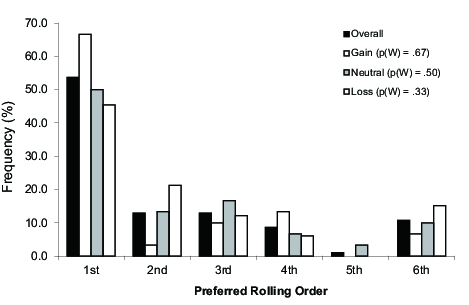
| Figure 5: Distributions of rolling order preference in Study 3. |
However, this effect might occur because of misestimation of the winning
probability, that is, early rolls are perceived as having higher winning
probabilities than late rolls, rather than because of uncertainty
aversion. To test this account, we analyzed participants’ estimates of
winning probability with a 3(game valence: gain vs. neutral vs. loss) x
3(roll order: first vs. third vs. last) mixed ANOVA. The results showed
that only the main effect of game valence was significant
(Mgain = .65 vs.
Mneutral = .46 vs. Mloss
= .32; F(2, 90) = 129.08, p < .001, ηp2
= 0.74). Neither the main effect of roll order
(Mfirst = .48 vs. Mthird
= .49 vs. Mlast = .47; F(2, 180) =
2.27, p = .106, ηp2 = 0.03) nor the interaction,
(F(4, 180) = 1.50, p = .203, ηp2 = 0.03) was
significant. This result implies that participants understood the winning
probability correctly and recognized that the rolling order did not induce
any change in the winning probability in all three conditions. This finding
also implies that participants favor early rolls even though they were
aware of the lack of a relationship between rolling order and winning
probabilities. In summary, early rolls are preferred to later ones even in
a game with replacement and this effect is not related with probability
misestimation.
Reasons for order preference. Similar with Study 1, two judges
categorized the stated reasons for preference into three types of
motivational factors and four types of probability estimation. Table 4
presents the results. First, a multiple regression7 was conducted to test the
relationship between each reason and preferred order. The results showed
that only uncertainty aversion was significant, β= –.39,
t(86) = 3.81, p < .001, thereby indicating that
uncertainty aversion alone affects rolling order preference in games with
replacement. This outcome is consistent with our expectation that the
simplicity of games with replacement lessens probability misestimation and
aversion to ambiguity and uncontrollability. Second, the third column
revealed that a major portion of participants mentioned uncertainty
aversion (43%) and no relationship between rolling order and winning
probabilities (53%) as the reasons for their choices. By contrast, only
a few mentioned ambiguity aversion, uncontrollability aversion, and
early/middle/late draw advantage. This finding is in line with the multiple
regression results. For more detailed analyses, a series of chi-square
tests examined whether a certain reason is associated with game valence
only for “uncertainty aversion” and “order is not related” statements that
satisfied the assumptions for chi-square tests. The analyses revealed that
both reasons were mentioned with a similar frequency across all the game
valence (χ2(2, N=93) < 3.21, p > .201, φ < 0.19). These
chi-square results generally support our contention that probability
misestimation hardly occurs in games with replacement.
| Table 4: Stated reasons for preferred play order as a function of game valence in Study 3. |
| | | Percentage (frequency) of participants who mentioned the reason for preference |
| | Regression β | Total | Gain | Neutral | Loss |
| Motivational Factors | | | | | |
| Uncertainty aversion | β = –.39* | 43% (40) | 47% (14) | 30% (9) | 52% (17) |
| Ambiguity aversion | β = .15 | 5% (5) | 10% (3) | 7% (2) | 0% (0) |
| Uncontrollability aversion | β = –.07 | 5% (5) | 0% (0) | 17% (5) | 0% (0) |
| Probability Estimation | | | | | |
| Early draw advantage | β = –.14 | 3% (3) | 3% (1) | 3% (1) | 3% (1) |
| Middle draw advantage | β = .02 | 2% (2) | 3% (1) | 3% (1) | 0% (0) |
| Late draw advantage | N.A | 0% (0) | 0% (0) | 0% (0) | 0% (0) |
| Order is not related | β = –.11 | 53% (49) | 57% (17) | 40% (12) | 61% (20) |
| Note. Regression betas are standardized beta coefficients from a
multiple regression analysis that tests the relationship between each type
of reason and preferred order. The number of participants is in parentheses.
*p < .05. |
5 General Discussion
The results of the three studies reveal biases in preference for playing
order in the context of a game with and without replacement. Both
motivational forces and biased probability perceptions affect these
preferences. For games without replacement, Studies 1 and 2 show that
early draws were preferred and this tendency was related to the
motivational factors such as uncertainty, ambiguity, and uncontrollability
aversions. Further, such a preference was modified according to game
valence. A gain game strengthened the tendency to prefer earlier draws,
whereas a loss game weakened it. This moderating effect was related to the
misestimation of winning probability. However, game valence did not affect
preference for early draws in games with replacement (Study 3), which
implies that uncertainty aversion that is not related to probability
estimation is a main motivational factor that leads people to favor early
draws.
Understanding decision making in games with and without replacement
provides insight into how people make decisions under uncertainty.
Research on human decision making has used various types of games and
gambles. For example, Ellsberg (1961) has demonstrated ambiguity aversion
by comparing games in which the exact numbers of balls of different colors
are known versus unknown. Bar-Hillel (1973) has devised gambles consisting
of compounds of simple gambles to present the conjunction fallacy.
However, little attention has been directed at decision making biases in
games with and without replacement. In particular, examining the judgment
biases in a no-replacement game expands the scope of the research on
decision under uncertainty. Such a game allows for the winning probability
to be changed by the outcomes of earlier draws and further complicates the
probability estimation. This characteristic is in contrast to a typical
two-gamble choice setting with a simple one-shot decision without
co-participants.
This study demonstrates that the factors driving the biased order
preferences are both motivational and cognitive. Previous
research on decision biases has focused mostly on either motivational
forces or cognitive forces. For example, Kahneman and Tversky (1982) have
differentiated between errors of comprehension and errors of application.
That is, biases are ascribed to either an incorrect understanding of a
decision problem (errors of comprehension) or incorrect decisions despite
a correct understanding of a problem (errors of application). This work
suggests that both comprehension and application errors affect the draw
order preference, specifically in the no-replacement game context.
The results of this study provide further insights into human decision
making and behavior in situations where people compete for limited
resources and opportunities, such as gambling and investment decisions.
For example, this work contributes to understanding people’s behavior when
buying apartments in South Korea. The funding for building large apartment
complexes in South Korea is unique. A construction company pre-sells the
rights of residency in new apartments before construction begins. The
specific apartment that each buyer receives in a housing complex is
decided by lottery when the construction is nearly complete. The
interesting point is that the apartments are not equally desirable. The
apartments located on higher floors and facing south represent “premium
housing” and are strongly preferred to ones located on lower floors and
facing north. Thus, premium housing is similar to the winning balls in
games without replacement. Like a no-replacement game, once a specific
apartment is picked by a buyer, it cannot be returned to the lottery.
Although the drawing order makes no difference in determining how likely
the home buyer will receive a desirable apartment, South Koreans line up
several hours before the lottery starts to draw lots as early as possible.
Preference for playing order in a game without replacement can also be
observed in gambling involving no replacement. One example is the game of
blackjack, in which whether the players’ win or lose is determined by the
cards they receive. In blackjack, players receive two cards from a deck of
shuffled cards, and the drawn cards are not replaced until the next
shuffle. Therefore, this situation is similar to a game without
replacement. Our theory predicts that people prefer to draw early (late)
when the remaining cards in the deck are more (less) favorable. People
(N = 182) who were familiar with the blackjack game participated
in a short survey. Participants were asked to imagine that they were at a
blackjack table where several plays had already been made after multiple
decks of cards had been shuffled and there would be several more plays
until the next shuffle. In the gain valence condition, participants were
informed that many favorable cards (10, J, Q, K, and A) had not been drawn
yet (i.e., a higher chance of receiving favorable cards). In the loss
valence condition, participants were informed that many favorable cards had
already been drawn (i.e., a lower chance of receiving favorable cards). The
results showed that the average playing position was significantly earlier
in the gain condition than in the loss condition
(Mgain = 2.71 vs. Mloss
= 3.07; F(1, 180) = .035, d = .31). This result indicated
that the valence of a game also affected the preference for playing order
in a gambling situation.
Despite these implications, the current research has limitations that
future research can improve. First, the three empirical studies examined
the hypotheses in the game context. Showing the effects only in a
particular situation can undermines the external validity of scientific
research. Future research may test the hypotheses in real life contexts
other than games to assess the robustness of the effect. Second, the
method for identifying the underlying mechanisms lacked rigorousness,
because we relied only on the analyses of the open-ended questions asking
the reasons for choices. Future research may elaborate more on the study
design to find evidence for the proposed mechanism. For example, highly
optimistic people are less ambiguity averse than less optimistic people
(Pulford, 2009). If future research measures optimism and finds the
relation between optimism and preference for early draws, then it may
corroborate our contention. Third, the sample size of Study 3 (games with
replacement) was relatively small despite being larger than the minimum
requirement. One may argue that the small sample size caused the
nonsignificant effect of game valence. Thus, reexamining the effect of
game valence with additional samples to obtain reliable results would be
worthwhile.
Another avenue for future research is to investigate the potential
moderating factors that may strengthen or weaken the biases. Individual
difference variables worth exploring include rationality, the need for
cognition, numeracy, and statistical training (Cacioppo & Petty, 1982;
Peters et al., 2006; Stanovich & West, 2008). For example, the bias
exhibited by a person with a strong need for cognition may stem from an
error of application, whereas the counterpart exhibited by a person with a
weak need for cognition is likely to stem from an error of comprehension.
Additional research can focus on ways to reduce judgment biases. The
effective bias-reducing methods can also depend on individual
characteristics such as their capabilities and traits. For instance,
methods to attenuate motivational forces such as uncertainty, ambiguity,
and uncontrollability aversion would be useful for persons who score low
on rationality measures, whereas methods to reduce probability
misestimation should be effective for persons who score high on such
measures.
References
Bar-Hillel, M. (1973). On the subjective probability of compound events.
Organizational Behavior and Human Performance, 9(3), 396–406.
https://doi.org/10.1016/0030-5073(73)90061-5.
Bordalo, P., Coffman, K., Gennaioli, N., & Shleifer, A. (2016).
Stereotypes. The Quarterly Journal of Economics, 131(4),
1753–1794. https://doi.org/10.1093/qje/qjw029.
Brown, E. R., & Bane, A. L. (1975). Probability estimation in a chance
task with changing probabilities. Journal of Experimental
Psychology: Human Perception and Performance, 1(2), 183–187.
https://doi.org/10.1037/0096-1523.1.2.183.
Cacioppo, J. T., & Petty, R. E. (1982). The need for cognition.
Journal of Personality and Social Psychology, 42(1), 116–131.
https://doi.org/10.1037/0022-3514.42.1.116.
Calvo, M. G., & Castillo, M. D. (2001). Selective interpretation in
anxiety: Uncertainty for threatening events. Cognition and
Emotion, 15(3), 299–320. https://doi.org/10.1080/02699930126040.
Camerer, C., & Weber, M. (1992). Recent developments in modeling
preferences: Uncertainty and ambiguity. Journal of Risk and
Uncertainty, 5(4), 325–370. https://doi.org/10.1007/BF00122575.
Cutright, K. M. (2012). The beauty of boundaries: When and why we seek
structure in consumption. Journal of Consumer Research, 38(5),
775–790. https://doi.org/10.1086/661563.
Cutright, K. M., & Samper, A. (2014). Doing it the hard way: How low
control drives preferences for high-effort products and services.
Journal of Consumer Research, 41(3), 730–745.
https://doi.org/10.1086/677314.
Denes-Raj, V., & Epstein, S. (1994). Conflict between intuitive and
rational processing: When people behave against their better judgment.
Journal of Personality and Social Psychology, 66(5), 819–829.
https://doi.org/10.1037/0022-3514.66.5.819.
Ellsberg, D. (1961). Risk, ambiguity, and the Savage axioms.
Quarterly Journal of Economics, 75(4), 643–669.
https://doi.org/10.2307/1884324.
Gilovich, T., Griffin, D., & Kahneman, D. (2002). Heuristics and
Biases: The Psychology of Intuitive Judgment. New York: Cambridge
University Press.
Gneezy, U. (1996). Probability judgments in multi-state problems:
Experimental evidence of systematic biases. Acta Psychologica,
93(1–3), 59–68. https://doi.org/10.1016/0001-6918(96)00020-0.
Gneezy, U., List, J. A., & Wu, G. (2006). The uncertainty effect: When a
risky prospect is valued less than its worst possible outcome. The
Quarterly Journal of Economics, 121(4), 1283–1309.
https://doi.org/10.1093/qje/121.4.1283.
Gregory, W. L., Cialdini, R. B., & Carpenter, K. M. (1982). Self-relevant
scenarios as mediators of likelihood estimates and compliance: Does
imagining make it so? Journal of Personality and Social
Psychology, 43(1), 89–99. https://doi.org/10.1037/0022-3514.43.1.89.
Güney, Ş., & Newell, B. R. (2015). Overcoming ambiguity aversion through
experience. Journal of Behavioral Decision Making,
28(2), 188–199. https://doi.org/10.1002/bdm.1840.
Howell, W. C. (1971). Uncertainty from internal and external sources: A
clear case of overconfidence. Journal of Experimental Psychology,
89(2), 240–243. https://doi.org/10.1037/h0031206.
Kahneman, D., Slovic, P., & Tversky, A. (1982). Judgment under
Uncertainty: Heuristics and Biases. New York, NY: Cambridge University
Press.
Kahneman, D., & Tversky, A. (1972). Subjective probability: A judgment of
representativeness. Cognitive Psychology, 3(3), 430–454.
https://doi.org/10.1016/0010-0285(72)90016-3.
Kahneman, D., & Tversky, A. (1979). Prospect theory: An analysis of
decision under risk. Econometrica, 47(2), 263–292.
Kahneman, D., & Tversky, A. (1982). On the study of statistical
intuitions. Cognition, 11(2), 123–141.
https://doi.org/10.1016/0010-0277(82)90022-1.
Langer, E. J. (1975). The illusion of control. Journal of
Personality and Social Psychology, 32(2), 311–328.
https://doi.org/10.1037/0022-3514.32.2.311.
Loewenstein, G. (1994). The psychology of curiosity: A review and
reinterpretation. Psychological Bulletin, 116(1), 75–98.
https://doi.org/10.1037/0033-2909.116.1.75.
Lovallo, D., & Kahneman, D. (2000). Living with uncertainty:
Attractiveness and resolution timing. Journal of Behavioral
Decision Making, 13(2), 233–250.
https://doi.org/10.1002/(SICI)1099-0771(200004/06)13:2<179::AID-BDM332>3.0.CO;2-J.
Newman, G. E., & Mochon, D. (2012). Why are lotteries valued less?
Multiple tests of a direct risk-aversion mechanism. Judgment and
Decision Making, 7(1), 19–24.
Peters, E., Västfjäll, D., Slovic, P., Mertz, C.K., Mazzocco, K., &
Dickert, S. (2006). Numeracy and Decision Making. Psychological
Science, 17(5), 407–413. https://doi.org/10.1111/j.1467-9280.2006.01720.x.
Pulford, B. D. (2009). Short article: Is luck on my side? Optimism,
pessimism, and ambiguity aversion. Quarterly Journal of
Experimental Psychology, 62(6), 1079–1087.
https://doi.org/10.1080/17470210802592113.
Sherman, S. J., Cialdini, R. B., Schwartzman, D. F., & Reynolds, K. D.
(1985). Imagining can heighten or lower the perceived likelihood of
contracting a disease: The mediating effect of ease of imagery.
Personality and Social Psychology Bulletin, 11(1), 118–127.
https://doi.org/10.1177/0146167285111011.
Shojaee, M., & French, C. (2014). The relationship between mental health
components and locus of control in youth. Psychology, 5(8),
966–978. https://dx.doi.org/10.4236/psych.2014.58107.
Simonsohn, U. (2009). Direct risk aversion: Evidence from risky prospects
valued below their worst outcome. Psychological Science, 20(6),
686–692. https://doi.org/10.1111/j.1467-9280.2009.02349.x.
Stanovich, K. E., & West, R. F. (2008). On the relative independence of
thinking biases and cognitive ability. Journal of Personality and
Social Psychology, 94(4),
672–695. https://doi.org/10.1037/0022-3514.94.4.672.
Tentori, K., Crupi, V., & Russo, S. (2013). On the determinants of the
conjunction fallacy: Probability versus inductive confirmation.
Journal of Experimental Psychology: General, 142(1), 235–255.
https://doi.org/10.1037/a0028770.
Tversky, A. & Kahneman, D. (1981). The framing of decisions and the
psychology of choice. Science, 211(4481), 453–458.
https://doi.org/10.1126/science.7455683.
Appendix A: Separate analyses of two games in Study 2.
| | 21.5inProbability of winning
(orange/white balls) | Game1 decision | Game2 decision |
|
Draw turn | | Draw | Defer | Draw | Defer |
| 1 | 50% (3/3) | 88% | 12% | 67% | 33% |
| | | (14) | (2) | (14) | (7) |
| | | χ2(1, N=16) = 9.00** | χ2(1, N=21) = 2.33 |
| | | φ = 0.75 | φ = 0.33 |
| 2 | 40% (2/3) | 58% | 42% | 36% | 64% |
| | | (7) | (5) | (5) | (9) |
| | 60% (3/2) | 78% | 22% | 80% | 20% |
| | | (7) | (2) | (8) | (2) |
| | | χ2(1, N=21) = .88 | χ2(1, N=24) = 4.61** |
| | | φ = 0.20 | φ = 0.44 |
| 3 | 25% (1/3) | 50% | 50% | 40% | 60% |
| | | (3) | (3) | (2) | (3) |
| | 50% (2/2) | 89% | 11% | 70% | 30% |
| | | (8) | (1) | (7) | (3) |
| | 75% (3/1) | 100% | 0% | 100% | 0% |
| | | (3) | (0) | (5) | (0) |
| | | χ2(2, N=18) = 4.18 | χ2(2, N=20) = 4.29 |
| | | φ = 0.48 | φ = 0.46 |
| 4 | 33% (1/2) | 50% | 50% | 56% | 44% |
| | | (5) | (5) | (5) | (4) |
| | 67% (2/1) | 100% | 0% | 100% | 0% |
| | | (5) | (0) | (9) | (0) |
| | | χ2(1, N=15) = 3.75* | χ2(1, N=18) = 5.14** |
| | | φ = 0.50 | φ = 0.53 |
| 5 | 50% (1/1) | 89% | 11% | 100% | 0% |
| | | (8) | (1) | (10) | (0) |
| | | χ2(1, N=9) = 5.44** | N.A |
| | | φ = 0.78 | |
| Note: Overall, the pattern of each game was similar to the aggregate data
analyses reported in the article. However, some tests results were not
significant. This is due to a lack of statistical power with a smaller
sample size when the data are separated into two games. Moreover, nearly
all the tests violated the assumption of the chi-square test, which
requires a minimum of five observations per cell. It is noteworthy that
all the effect sizes were greater than 0.20. |
| * p < .10, ** p < .05. |
This document was translated from LATEX by
HEVEA.