Judgment and Decision Making, Vol. 16, No. 4, July 2021, pp. 1072-1096

Abstract: A standard way to elicit expectations asks for the percentage chance an event will occur. Previous research demonstrates noise in reported percentages. The current research models a bias; a five percentage point change in reported probabilities implies a larger change in beliefs at certain points in the probability distribution. One contribution of my model is that it can parse bias in beliefs from biases in reports. I reconsider age and gender differences in Subjective Survival Probabilities (SSPs). These are generally interpreted as differences in survival beliefs, e.g., that males are more optimistic than females and older respondents are more optimistic than younger respondents. These demographic differences (in the English Longitudinal Study of Ageing) can be entirely explained by reporting bias. Older respondents are no more optimistic than younger respondents and males are no more optimistic than females. Similarly, in forecasting, information is obscured by taking reported percentages at face value. Accounting for reporting bias thus better exploits the private information contained in reports. Relative to a face-value specification, a specification that does this delivers improved forecasts of mortality events, raising the pseudo R-squared from less than 3 percent to over 6 percent.

Keywords: subjective probabilities; subjective survival probabilities; expectations; gender differences; survey biases

1  Introduction

Expectations are core to decision making. Substantial resources are spent eliciting subjective expectations. For example, The Federal Reserve Bank of New York launched a Survey of Consumer Expectations (SCE) in 2013. Many surveys, including the SCE and the Health and Retirement Survey, elicit expectations by asking respondents to report the percentage chance that some outcome will be realized. Also, in life generally, people often solicit opinions by asking for a percentage. For example, in an interview, Tyler Cowen asks music critic Alex Ross “if you …go to the opera, what percentage of the crowd there is actually enjoying it in the sense that they are wishing it would last longer than it will?” (Cowen, 2020).

It has long been established that there are systematic biases in probabilistic beliefs. In general, people act as though they believe a one percentage point increase in risk to be larger when it occurs in the tails of the distribution than when it occurs in the middle of distribution. This bias in beliefs leads to preference reversals such that people overinvest in protecting themselves against low probability events (e.g., Allais, 1953; Slovic, 1987). Such biases in beliefs will manifest when people are asked to report their likelihood judgment as a percentage chance (e.g., Ludvig & Zimper, 2013; Lee & Danileiko, 2014). The current research considers a separate and additional source of bias in reported percentages, one that has very different implications for predicting respondent behavior. In what follows, I exploit demographic variations in objective life expectancy and variations in the subjective survival probability questions asked of a representative sample to parse biases in belief from biases in the reporting of those beliefs. The distiction between biased beliefs and biased reports matters. For instance, a review on the psychology of pensions investment reports: “First, individuals tend to be overly pessimistic when thinking about the likelihood of dying at younger ages (e.g., before age 75) and overly optimistic about surviving into older ages. Second, women tend to underestimate their life expectancies more than men do” (Shu, 2021, p. 2). The current research investigates whether these age and gender differences represent differences in optimism or whether they are merely response biases to a question that happened to be asked in a survey. Differences in optimism would be expected to influence planning for retirement whereas a survey response bias to a specific question would not.

The current research proposes a non-linear mapping from subjective likelihood beliefs onto reported percentages: a five percentage point change in reported probabilities implies a larger change in beliefs at certain points in the probability distribution. This non-linearity induces a bias because error is no longer independent of beliefs. Accounting for reporting bias will recover a less contaminated representation of respondents’ private beliefs. This insight can improve forecasting. First, at the micro-level, a cleaner measure of an individual’s beliefs will better predict choices and behaviors. Second, at the macro-level, the wisdom-of-the-crowd can be leveraged if the crowd’s beliefs are measured devoid of systematic bias. By stripping away reporting bias, it should be possible to better predict objective outcomes.

This research contributes to various literatures, most specifically that on subjective survival beliefs. Using data from the English Longitudinal Study of Ageing (ELSA), I demonstrate that two demographic effects that are widely interpreted as differences in survival beliefs are manifestations of reporting bias. Whereas the previous literature reports men to be more optimistic in their survival beliefs than women, I demonstrate that for any given objective survival probability male respondents hold subjective beliefs that are no more optimistic than female respondents. And, whereas the previous literature reports older respondents to be more optimistic in their survival beliefs than younger respondents, my reanalysis of the ELSA data shows no age effect in beliefs. The demographic effects appear because men and older respondents are asked about events that are objectively less likely than the events that women and younger respondents are asked about. Curvature in the function that maps beliefs onto reported percentages means that men and older respondents report percentages that are especially positively divergent from objective survival probabilities.

This research also contributes to the literature on expectations measurement generally. Parsing between beliefs and reporting bias allows researchers to identify more cleanly beliefs and belief-updating processes (e.g., Armantier et al., 2013). So, in the current context, the insight that demographic differences in reported survival probabilities are artefacts of measurement rather than differences of belief obviates the need to “debias” longevity beliefs (e.g., Comerford & Robinson, 2020; O’Dea & Sturrock, 2020). Moreover, this research contributes to the literature on expectations elicitation. The biases and ambiguities revealed here recommend research to find less bias-prone measures than those that elicit a percentage chance.

Finally, this research contributes to the forecasting literature. It demonstrates data transformations that can be applied to reported percentages that would generally be expected to improve predictive power.

This is not the first paper to recommend transforming reported percentages. There is an extensive literature that recommends transformations as a means to redress judgment biases and hence improve forecast accuracy (e.g., Lee & Danileiko, 2014; Steyvers et al., 2014; Turner et al., 2014). Note that the goal of the current research is substantively different from these papers, which sought to mitigate judgment biases; it is to recover cleaner measures of respondents’ beliefs (regardless whether those beliefs are accurate or not).

The current research is most closely related to a set of papers that seek to account for response biases in the reporting of percentages. Based on the insight that respondents report specious 50 percent responses, Bruine de Bruin et al. (2002) redistributed excess 50% responses to points in the probability distribution where responses were anomalously infrequent relative to a smooth distribution. Karvetski et al. (2013) and Fan et al. (2019) employ a coherentization procedure. If a respondent reported two complementary probabilities that sum to more than one then coherentization imposes a sum of one and rescales each individual probability accordingly.

The transformations I apply are different. One employs rank information and the other introduces a quadratic term. Both are recommended by a model that describes reported percentages as non-linear transformations of likelihood beliefs¹. Unlike Bruine de Bruin et al.’s approach, these transformations can improve forecasting even when each respondent is forecasting a respondent-specific outcome, such as their own mortality. Unlike coherentization, these transformations can be applied even when each respondent reports only one percentage.

I test my transformations against a specification that takes reported probabilities at face value in longitudinal data. A useful feature of these data is that they give thousands of individual forecasts that can be validated against thousands of individual survival/mortality events. Both of my data transformations better predict mortality than the specification that takes survival probabilities at face value.

1.1  Model

The empirical analyses that follow consider subjective survival probabilities (SSPs) and so I take as a motivating example for this theory section SSPs. Many longitudinal ageing studies (e.g., ELSA in England, the Health and Retirement Survey [HRS] in the US, Survey of Health Ageing and Retirement in Europe [SHARE]) elicit subjective survival probability distributions by asking for the percentage chance that the respondent will live to some target age. These questions deliver an observable percentage chance, Y_ij, that purports to measure respondent i’s latent belief regarding outcome j, x_ij. as

Researchers using SSP data have long recognized patterns in the data indicating that Y_ij differs from x_ij, a fact which is captured in equation 1 by a randomly distributed noise term, e_ij. The fact was inescapable to early users of HRS data, who observed that 43 percent of respondents answered these questions with either 0%, 50% or 100% (Hurd, 2009). The literature is split on how to deal with this empirical anomaly. Some press on regardless, treating raw reports of percentage chance as the best available approximation of beliefs (e.g., Elder, 2013). Some have attempted to account for measurement error in mortality beliefs by dropping suspect-looking observations from the data. This approach is marred by difficulties identifying which responses are to be kept as signaling private information and which are to be dropped as meaningless noise. Salm (2010, p. 1043) dropped respondents who reported a 0% percent chance of surviving a further decade but kept those who reported a 100% chance, whereas O’Dea and Sturrock (2018, p. 28) did precisely the opposite. Some have sought to navigate around the issue by using an instrumental variables approach (e.g., Delavande et al., 2006; Bloom et al., 2006; Bíró, 2013). For instance, Bíró (2013) takes the death of a respondent’s sibling to be an exogenous shock to survival beliefs and uses this instrument to answer whether consumption is sensitive to subjective survival probability. A cost of this approach is that it relies on an average treatment effect and so fails to exploit the individual-level private information that is a key advantage of survey data.

The current research takes a different approach. It models Y_ij as a manifestation of x_ij that is systematically distorted by reporting bias, r_ij:

An advantage of this approach is that it neither throws away any observations nor imposes such restrictive assumptions as the instrumental variables approach. As such, it makes richer use of potentially diagnostic private information than do many previous attempts to account for measurement error. Harnessing this private information is especially useful in the domain of SSPs because each respondent is forecasting a respondent-specific outcome (their own survival) about which they have rich and meaningful data e.g., the age of death of genetic relatives; their health-relevant behaviours; their current state of physical health.

The key question then is what form does r_ij take? The literature demonstrates that some respondents i report uninformative responses and these tend to cluster at 50%. This tendency has been explained as respondents using 50% to indicate “I have no idea” (Fischhoff & Bruine de Bruin, 1999). A stark example of this phenomenon is reported in Hurd (2009), where respondents reported a 50% chance of living to age 75 and immediately afterwards answered that they did not believe that it was as likely as not that they would survive to age 75. This result demonstrates that misreporting of beliefs is commonplace: this contradictory pattern of response was demonstrated by 63 percent of those who answered 50%, which was 23 percent of the total HRS sample in that wave of data collection. On that basis alone, roughly one in six respondents to the HRS answered with a percentage that was closer to 50% than they believed their survival probability to be.

The results of Fischhoff and Bruine de Bruin (1999) and Hurd (2009) also demonstrate that this response bias differs within respondents i across domains j. Hurd (2009) reports that contradictions were even more common when the same sample of HRS respondents was asked for a percentage chance of the stock market going up over the coming year than when asked about the probability of living to some given age.

These uninformative 50% responses can introduce bias when they interact with features of question wording. Notably, SSP questions vary the target age that respondents are asked about. Because a 50% chance of living to an older target age implies a longer life expectancy than a 50% chance of living to a younger age, these uninformative responses can give a mistaken impression of respondent beliefs. I consider this in greater detail in Study 2.

A second description of r_ij suggested by the literature concerns the use of scale endpoints. Merkle et al. (2016, p. 16) write of the “overuse” of 0% and 100% in their data, which comes from a US sample. This might be explained by certain respondents having a tendency to use the extreme points on any response scale, what Paulhus (1991) terms “extremity response bias” and van Vaerenbergh and Thomas (2013) term an “extreme response style”. Whether scale endpoints are overused or underused seems to vary across nations and cultures. In an English sample, Oswald (2008) finds a reluctance to use scale endpoints. He compares reports of respondents’ own height on a subjective scale (i.e., a ten-point scale labelled “very short” and “very tall” at either end) to objective measures of their height. He finds a bias in the mapping from beliefs onto the response scale. The subjective measure was highly correlated with the objective measure but was insufficiently sensitive to gradations in actual height, particularly at the scale endpoints. As such, response bias implied very tall and extremely tall respondents to be more similar in height than these respondents’ believed themselves to be. This reluctance to use scale endpoints among English respondents might reflect a general tendency to avoid scale endpoints; what Vaerenbergh and Thomas (2013) term a “mid-point response style”. If so, it might explain an anomaly in reported probabilities across English and Irish samples. When asked for SSPs regarding surviving 11–15 years into the future, just 6 percent of English respondents to ELSA answered 100% compared to over 30 percent of Irish respondents (Bell et al., 2020). The authors suggest cultural differences as a potential mechanism driving this divergence.

The results of Oswald (2008) demonstrate respondents’ reports can be systematically higher or lower than their beliefs and that this is especially true in the tails of the distribution. Various results suggest that this insight applies to reported probabilities (e.g., Merkle et al., 2013; Bell et al., 2020) with the result that the bias term r_ij is larger if the respondent’s belief x_ij is especially high or especially low.

To the extent that reporting bias varies systematically with likelihood beliefs, it is overly restrictive to interpret reported percentages as a linear translation of respondents’ likelihood beliefs. Inferences regarding beliefs that rely on a linear interpretation may be mistaken. For example, if A overestimates a survival probability by 10% and B overestimates a different survival probability by 8% it may not be true that A holds more optimistic survival beliefs than B. To compare survival optimism, we should compare estimates for the same survival event.

1.2  Data

Four of the five analyses presented in what follows employ data from ELSA, a survey of older English people’s experience of aging (ELSA, undated). Data is collected via in-person interviews. ELSA recruited a representative sample of English households aged 50 and over for its first wave, in 2002. It has since followed up with its panel members every second year. With each wave, new households are recruited into the sample to replace respondents who have died or who do not respond when contacted. My tests for the robustness of age and gender effects employ data from Wave 7 of ELSA, fieldwork for which was conducted in 2014–2015. I use this wave of data because the ONS published life tables for the English population for that same year 2015 (ONS, undated). Two of my analyses exploit the longitudinal dimension of ELSA and so use data from Waves 5 (2010–2011) through to Wave 8 (2016–2017).

The first analysis I present derives from a distinct longitudinal study of ageing, SHARE, that employs standardized data collection across many European countries and Israel (SHARE, undated).

2  Studies 1: Reporting Bias Explains Gender Differences in SSPs

This part of the paper comprises two tests. The first tests for and finds cultural differences in the likelihood of reporting 0% and 100%. That result implies non-linearities in the mapping from beliefs to reported percentages. It may be then that differences in survival optimism across males and females are overstated. The main test in this section investigates whether gender effects persist when males and females are judging survival events of identical objective probability.

2.1  Evidence of cultural differences in the likelihood of reporting 0% and 100%

Wave 2 of the SHARE (Survey of Health and Retirement in Europe) study recruited over 1000 respondents representative of the over-50s in their national population from 15 countries. A standardised instrument and data collection protocol were used across 14 European countries and Israel. The total sample size is 37,512. Data were collected in 2006 (SHARE, undated).

All respondents were asked the SSP question “What are the chances that you will live to be age [75/80/85/90/95/100/105/110/120] or more?” The target age in the question was 11–15 years older than the respondent’s current age.

On average across the entire sample, 14.1 percent of respondents answered 100% but the likelihood of doing so ranged from 4.8 percent in the Czech Republic to 24.8 percent in Ireland. Five percent of the total sample reported a 0% chance of living to a target age but the likelihood ranged from 1.6 percent in Greece to 9.8 percent in Poland.²

These large differences in the use of scale endpoints were often at odds with objective conditions – in Denmark 24 percent reported 100% but in Belgium just 8.2 percent did, even though the CIA world factbook for 2006 estimated life expectancy in Denmark to be a year lower in Denmark than in Belgium (CIA, 2006). They are also inadequately explained by cultural differences in optimism. If that were the explanation then we would expect to see a high negative correlation between the likelihood of reporting 100% and the likelihood of reporting 0%. In fact the observed correlations are low, ranging from r =−.042 (Greece) to r= −.125 (Ireland).

These results suggest national differences in willingness to report 0% and 100%. This result implies that in some countries a very low likelihood belief is reported as zero where in others that same belief is reported as some positive percent. In other words, there are non-linearities in the mapping from beliefs to reports.

2.2  Are Gender Differences in Survival Beliefs Robust?

Previous research has reported that, relative to life tables, women underestimate their objective likelihood of living to a given age to a greater extent than do men for the nine European countries that issued the SHARE survey (e.g., Perozek, 2008 for the USA; Wu et al., 2015 for Australia; de Bresser 2019 for the Netherlands; Bell et al., 2020 for England and Ireland; Philipov & Scherbov, 2020 for the nine European countries that issued the SHARE survey). This pattern of results is consistent with the broader literature on gender differences in response to risk and uncertainty, which finds men to be more optimistic and more likely to exhibit overconfidence (Charness & Gneezy, 2012).

The previous test suggests that the observed gender difference might be, at least in part, an artefact of how SSP is elicited. Specifically, it shows a non-linearity in the mapping from beliefs to reported percentages. In the English data that is the object of the current analysis, the available data suggest a reluctance to report responses of 0% and 100% (Oswald, 2008; Bell et al., 2020). On average in England, women live longer than men. An obvious but underappreciated feature of asking women and men about living to some given target age is that the objective probability of women making it to that target age is higher than the objective probability of men making it to the same target age. To the extent that misreporting of percentages leads respondents to under-report high probability events, we would expect the scale of under-reporting to be greater for female respondents than for males, since female respondents are estimating even higher probability events than are male respondents. It might be then that this survey response mechanism partly explains widely reported gender effects in SSP.

2.3  Method

I test whether there remains a gender effect in likelihood reports after controlling for the objective probability of the event.

2.3.1  Participants

The sample comprises respondents to Wave 7 of ELSA, which draws from a representative sample of English households aged 50 and over. Data collection took place in 2014–2015.

2.3.2  Design

I compare the survival probabilities reported in UK life tables for the years 2014–2016 against the ELSA respondents’ SSPs.

2.3.3  Procedure

Procedure: Model 1

Looking at UK life tables for 2014–2016, the probability of a woman aged 69 living to age 80 is 79.51%. The probability is virtually identical for a man aged 61 of living to age 75, 79.50 (ONS, 2016). In 2014–2015, Wave 7 of ELSA asked 69 year-old women about their probability of living to 80 (n=221) and also asked 61 year-old men about their probability of living to 75 (n=151). I test whether there is a gender difference in the SSPs reported by these two groups, who were on average judging the likelihood of equally likely events. If gender differences are robust then we should see a negative coefficient on female, indicating that females estimated a lower likelihood of an event that is 79.5% likely to occur.

Procedure: Models 2 and 3

An alternative test of the same hypothesis that can be run on the entire sample is whether the scale of under-reporting is larger for women than for men after controlling for objective survival probability. The scale of under-reporting is measured as Subjective/Objective Discrepancy or SOD. It is measured by subtracting Objective Survival Probability from Subjective Survival Probability i.e., SSP−OSP. SOD would take a value of 5, for instance, if the respondent reports a probability of 90% of living to a given age and if life tables give a probability of 85% that someone of the respondent’s age and gender would live to that given age. At the level of any individual respondent, there might be sound reasons for SOD to differ from zero. For example, SOD should be a negative number if a respondent has received a terminal diagnosis. On average, however, SOD should be zero because ELSA recruits a representative sample of English households and so the average ELSA respondent would be expected to have the same survival probability as enumerated in mortality tables for the English population.

2.4  Results

Model 1, the first column of Table 1, reports the coefficients from the following OLS regression:

where the baseline category is male and the sample is limited to just those respondents whose age and gender implies an OSP of 79.5%. The model therefore tests whether being female predicts reported probabilities of a survival event that has expected probability of 79.5%. The coefficient on being female is not significant, indicating that there is no gender difference in estimates of this outcome.

---

Table 1: OLS regression of Survival Optimism on being female and Objective Survival Probability (OSP) given by population life tables.

	Model 1		Model 2		Model 3
	SSP of event	p-value	SOD	p-value	SOD	p-value
Female	1.608	.493	−3.851	<.001	0.182	.340
	(2.341)		(0.593)		(0.527)
OSP					-0.533	<.001
					(0.011)
Constant	63.730	<.001	2.152	<.001	29.24	<.001
	(3.905)		(0.968)		(1.005)
Observations	372		8694		8694
R-squared	0.00		0.005		0.232

Notes: Model 1 estimates an OLS Regression of Subjective Survival Probabilities for respondents whose Objective Survival Probability was given by mortality tables as 79.5%. Models 2 and 3 estimate an OLS Regression of Subjective/Objective Discrepancy, SOD. Standard errors in parentheses.

---

Model 2 reports the coefficients from the following OLS regression:

where the baseline category is male. SOD measures deviation from the objective value implied by life tables. Model 2 tests whether females deviate from their objective values to a greater extent than males deviate from their objective values. The previous literature has found a negative coefficient on female in such models, which is what we observe in Model 2 also (p<.001).

Model 3 reports the coefficients from the following OLS regression:

where OSP is the objective value determined by respondents’ age and gender. Because OSP varies by gender, controlling for it in the regression fixes the objective value across respondents. It allows like-for-like comparisons of the scale of deviations made by respondents of different genders. Model 3 therefore answers whether there is a gender difference in deviations from objective likelihoods when we hold constant objective likelihoods. It shows no reliable difference across men and women in the degree to which they underestimate an identical survival probability (p= .340).

Crucially, the coefficients on female across Models 2 and 3 differ significantly from one another (t= 5.08, p<.001), which demonstrates that the effect of gender on survival optimism is smaller than has been assumed in the previous literature.

2.5  Discussion

A gender effect that had been widely reported to be a difference in optimism across women and men was, at least in these data, a survey artefact. It was entirely explained by the fact that women were being asked about events that are objectively more likely than the events that men were being asked about. Because males and females both report percentages that become more biased in the tails of the distribution, females appeared to under-report the true probability to a greater extent than did men. This analysis demonstrates that previous research has overstated the degree to which women hold less optimistic survival beliefs than men.

3  Study 2: Are Age Effects in Survival Beliefs Robust?

The basis for this study is termed the “flatness bias” (Elder, 2013). It refers to the fact that SSPs are less sensitive to age than are objective survival probabilities (OSPs, as given by life tables). The flatness bias is depicted in Figure 1 and has been found in a range of national samples (e.g., Ludwig & Zimper, 2013 for the USA; Wu et al., 2015 for Australia; Steffen, 2009 for Germany; Douglas et al., 2020 for England and Ireland). Figure 1 graphs data from male respondents to ELSA Wave 7. The horizontal axis depicts respondents’ age at time of interview. The vertical axis charts the probability of living to some target age. The dashed lines depict OSPs and the full lines depict SSPs. OSPs are derived from ONS mortality tables (ONS, undated). The graphs show that the age decline in SSPs is systematically flatter than the age decline in OSPs i.e. a flatness bias.

---

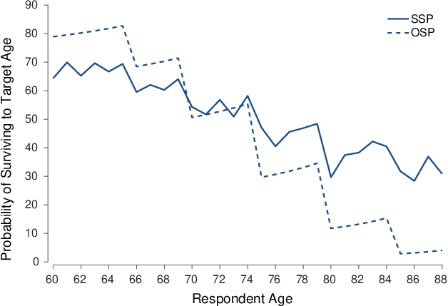
Figure 1: Data comparing subjective and objective probabilities of living to a given target age. SSPs from men in ELSA Wave 7 are shown by the solid line and OSPs from contemporaneous life tables are shown by the dashed line. Subjective probabilities show less of a response than Objective probabilities to changes in target age, as indicated by the discontinuities in the lines.

---

Eyeballing the graphs, the flatness bias is driven to a large extent by discontinuities in the survival rate at ages 70, 75, 80 etc. These discontinuities occur because the target age in the SSP question employed by ELSA increases at those ages. At ages where the target age in the question increases, subjective probability drops, but not by as much objective probability.

Many surveys of ageing that elicit SSPs do so by increasing the target age that respondents are asked about surviving to as respondents themselves age. Data from those other surveys exhibit the same pattern as depicted in Figure 1 i.e., SSP is less responsive to each increase in target age than is OSP. Ludwig and Zimper (2013, Figure 1) show this starkly for a US sample in HRS data. Bell et al. (2020, Figure 2) show it starkly for an Irish sample in TILDA.

Previous research has attributed the flatness bias to various biases in beliefs, such as a failure to recognize that mortality rates increase with age (Elder, 2013) or an initial lack of information that is corrected at older ages (Ludwig & Zimper, 2013). But the flatness bias would arise mechanically from uninformative responses.

Consider the case of a respondent who answers 50% to indicate “I have no idea” (Fischoff & Bruine de Bruin, 1999). When they are interviewed at age 69, a respondent reports a 50% chance of living to age 80. In the next wave of data collection, two years later, they again answer 50% to the SSP question, although this time they have been asked about the probability of living to 85. Relative to OSP, this respondent’s SSP has become more positive from one wave to the next for reasons that are totally unrelated to the respondents’ underlying survival beliefs. The upshot is that there will be a specious age effect when we analyse SODs.

The specious age effect will be most pronounced if the respondent always answers the SSP question with some fixed percentage. It can also derive from the nonlinear mappings from beliefs to reports that were the subject of Study 1. Any respondent who reports a percentage that is closer to 50% than the percentage they believe to be true will report SSPs that are less sensitive to increases in target age than are OSPs.

The discontinuities depicted in Figure 1 have important implications for interpretation of the coefficient on age (or more sophisticated transformations of age such as age-squared etc.) in a regression of SOD. That coefficient will pick up two independent effects: 1) a pure age effect, which measures the change in SOD that is associated with being a year older, and 2) a target age effect, which measures the change in SOD that results from the change in target age at certain age thresholds.

We can control for the effect of the change in target age. Including a dummy variable that indicates which target age the respondent was asked about in the regression of SOD will deliver a coefficient on age that is uncontaminated by shifts in target age. Table 2 reports for ELSA which target age respondents in each age range were asked about.

---

Table 2: Target age asked about in ELSA’s SSP Question by respondents’ own age.

Age of respondent	Target age asked about in SLE question
50–65	75
66–69	80
70–74	85
75–79	90
80–84	95

---

Study 2 follows the same template as Study 1. The core part of Study 2 demonstrates that flatness bias is not a manifestation of biased beliefs but is a manifestation of biased reports. Before that, I present novel evidence of uninformative responses by exploiting the longitudinal dimension of ageing studies.

3.1  Method

3.1.1  Participants

I use data from Waves 5, 6 and 7 of ELSA, fieldwork for which were conducted in 2010–2011, 2012–2013 and 2014–2015 respectively. There were 4795 respondents who met the criteria described in the procedure section.

3.1.2  Procedure

My criteria for an uninformative response are:

1. The respondent reported precisely the same SSP in three consecutive waves of data collection and that SSP was neither 0% nor 100%.
2. They did so despite being asked about a higher target age than they had been asked in a previous wave of the survey. For instance, some respondents will have aged from 67 to 71 between Waves 5 and 7. Accordingly, these respondents will have been asked about their probability of living to age 80 in Waves 5 and 6 and asked about living to age 85 in Wave 7. A response of x% looks uninformative if a respondent has a track record of answering x% whenever they have been asked about the probability of living to 80 and then they also answer x% when they are asked about the probability of living to 85. We might doubt the increase in life expectancy implied by their response to the target age 85 question.
3. They report no improvement in subjective health. Some of the respondents who meet criteria 1 and 2 may have experienced a positive health shock. That may have prompted them to increase their subjective life expectancy to such an extent that it was not unreasonable of them to report the same SSP for age 85 as they had earlier reported for age 80. We can test whether respondents perceived themselves to have experienced a health improvement from one wave to the next by looking at respondents’ answers to the subjective health questions in ELSA.

3.2  Results

Of the 4795 respondents that reported SSPs and subjective health in all three waves of data collection and also aged into an older target age category, 6.4 percent reported an identical SSP in all three waves of data collection despite being asked about a different target age in one of the waves. A minority of these (n = 77) concurrently reported an increase in subjective health, but the majority did not. All three criteria were satisfied in 4.8 percent of cases. Of these, a further 45 reported 0% or 100% across all three waves. These reports may be valid; if a respondent believes there is a 0% chance of living to 75 then they must also believe there is a 0% chance of living to 80. Similarly, if they believed that there was a 100% chance of living to 85 then, when asked about living to age 80 they would be correct to report 100%. Dropping these cases, 4.6 of the sample fits my criteria as uninformative. In about half of these cases (102 out of 185), the uninformative response was 50%. Uninformative responses of 50% have already been exposed in SSP reports (Hurd, 2009). Still, this analysis suggests that an additional 1.7 percent of responses to SSP questions are uninformative, over and above meaningless 50% responses.

These uninformative responses, in common with meaningless 50% responses, will mechanically deliver data that appear more optimistic as respondents age into higher target age categories. In what follows, I present three models to disentangle the effect of respondents’ age from the effect of target age. The first estimates the coefficient on age in a standard model. It regresses the SOD on respondent’s age in years and whether the respondent is female.

The second is a corrected model. It additionally controls for dummy variables indicating which specific target age the respondent was asked about.

The third model is a placebo test. A placebo test is necessary because the corrected model controls for target age by controlling for age category (e.g., 50–65; 66–69 etc., see Table 2). The coefficient on the target age dummies will therefore pick up two effects – the effect of target age and the effect of being in a given age category (e.g., 50–65). A concern with our corrected model is that age and age category are highly correlated; adding any age category as a covariate to a model that already includes age would, in itself, reduce the coefficient on age. Our placebo models estimate this age category-effect to rule out that it is age category, rather than target age, that is driving the results of the corrected model. In practice, we test the effect of controlling for age categories other than those that correspond with the discontinuities in target age. I ran four placebo models to test various age categories so that I mitigate the risk of using an unrepresentative estimate of the age category-effect (see Table 3).

The hypothesis is that these placebo tests demonstrate a reduction in the coefficient on age that is significantly smaller than that returned by the corrected model. The difference between the coefficients on age returned by the corrected model and by the placebo models is the effect of target age, net of any effect of age category.

Table 4 presents the results of the standard, corrected and placebo models. In each case, we are interested in the coefficient on age. The standard model is of the form SOD = a + b₁(age) + b₂(female), where the omitted category is male.

The corrected model is specified as

where target age is an indicator variable identifying which of the seven target ages the respondent was asked about the probability of living to (see Table 2).

The placebo model is specified as:

where age category is an indicator variable identifying which of seven age categories the respondent’s current age places them in (see Table 3).

---

Table 3: Age categories that were controlled for in each of our placebo tests.

Age Category	Placebo Model 1	Placebo Model 2	Placebo Model 3	Placebo Model 4
1	50–61	50–63	50–64	50–62
2	62–66	64–67	65–68	63–68
3	67–70	68–71	69–72	69–73
4	71–75	72–76	73–77	74–78
5	76–80	77–81	88–82	79–83
6	81–85	82–86	83–87	84–88
7	86–90	87–90	88–90	89–90

---

The standard model suggests a large positive age effect; SOD becomes 1.2 percentage points more positive with each additional year of life (t= 42.25, p<.001). In other words, each additional year of life is associated with reporting an increase of 1.2 percentage points in the probability of living to a given age, over and above the change in probability of living to that age recorded in ONS life tables. The corrected model, which additionally controls for target age, finds a small, negative age effect (b= −0.168, t=1.94, p= .0514).

The placebo models find smaller age effects than did the standard model but, crucially, they are all more positive than in the corrected model (see appendix). Table 4 reports the results of Placebo Model 3, which came closest to the corrected model i.e. it delivered the least positive coefficient on age (b= 0.197, t= 2.05, p=.041). Crucially, it delivered an age coefficient (b= 0.197) that was significantly more positive than the coefficient returned by the corrected model (b= −0.168, t= 2.83, p=.005). This significant difference in coefficients on age across the corrected and placebo model captures the effect of target age, net of age category. It supports my hypothesis that the positive effect of age on SOD is specious. The significant coefficient on age is induced by the increases in target age asked about in the survey instrument.

---

Table 4: Age effects on survival optimism are not robust.

	Standard Model		Corrected Model		Placebo Model 3
	Coefficient	p-value	Coefficient	p-value	Coefficient	p-value
Age	1.233	<.001	−0.168	.051	0.197	.041
	(0.029)		(0.086)		(0.096)
Female	−4.720	<.001	−5.281	<.001	−5.198	<.001
	(0.545)		(0.530)		(0.536)
Dummies for target age			Included	<.001
Dummies for seven age categories			Included	<.001
Constant	−80.397	<.001	3.879	.456	−18.298	<.001
	(2.173)		(5.199)		(6.457)
R2	0.18		0.23		0.21
N	8627		8627		8627
Notes: The table reports OLS regressions of SOD, i.e., the scale of discrepancy between subjective survival probabilities and objective survival probabilities. The Standard Model controls only for whether the respondent is female. The Corrected Model additionally controls for the target ages respondents were asked about their probability of surviving to. Placebo Model 3 tests whether the null effect of age found in Model 2 is explained by the fact that controlling for target age also happens to control for age category; Placebo Model 3 controls for arbitrary age categories. The coefficients on the dummy variables and all four placebo tests are presented in the online supplement. Standard errors in parentheses.

---

3.3  Discussion

The hypothesis that motivated this study was that flatness bias, or the age effect in SOD, is partially explained by the increasing target ages that are asked about in longitudinal studies of ageing. Ideally I would have randomly assigned target age since this would give a clean estimate of its causal effect on SOD. This was not possible. Instead I controlled for the target age. That had the additional effect of controlling for respondents’ age category. This raised the possibility that some of the effect that I attribute to target age might merely be an age category effect. To rule out this possibility I conducted placebo tests in which I controlled for arbitrary age categories. Regardless which age categories I controlled for, the age effect on SOD was only ever eliminated when I controlled for the age categories that are coterminous with target age. I conclude that the increase in target age as respondents’ age is the driver of flatness bias, in these data at least. In other words, younger respondents in Wave 7 of ELSA were no more pessimistic in their survival beliefs than were older respondents. This result matters because previous literature has interpreted the SSPs reported in ELSA data at face value. It concluded that the average younger respondent underestimated their objective survival probability to a greater extent than did the average older respondent (e.g., Bell et al., 2020; O’Dea & Sturrock, 2018) and made policy recommendations premised on that result (O’Dea & Sturrock, 2020).

4  Test of Predictive Power

To the extent that we can predict how SSPs deviate from beliefs, we should be able to recover more accurate belief measures. In this section I seek to do this by testing whether my model of response biases can lead to more accurate predictions of an objective outcome, death.

If we take SSPs at face value then we are accepting the percentage that respondents report as their best estimate of their likelihood of living for a further 11–15 years (i.e., to the target age that happened to be asked about in the question).

My model suggests that we can reconstruct a more accurate manifestation of respondents’ beliefs from their biased reports. Specifically it posits that a one percentage point difference in SSPs indicates a varying difference in beliefs contingent on whether beliefs are at the extremes of the probability distribution or in the middle of the distribution. Taking the example of UK data, where respondents appear reluctant to use scale endpoints, my model predicts that two respondents who report 45% and 40% likelihood of living to age 80 respectively have beliefs that are more similar to one another than two respondents who respectively report a 6% and 1% likelihood of living to age 80. One way to recover the discriminating power of SSPs reported in the tails of the distribution is to apply a quadratic term, as in the study of subjective height reported previously (Oswald, 2008). This would allow a one percentage point difference in the tails of the distribution to quantify something different than a one percentage point difference in SSPs closer to 50%.

A separate approach to recover the discriminating power of reported SSPs is to use them to generate a rank measure of likelihood of death. Let us take the example of a respondent who reports a 10% chance of dying at age 80 when 99 percent of respondents who were asked that same question reported a chance of dying at 80 of at least 11%. The hypothesis suggested by our model is that, given a general bias in the reporting of percentages, the fact that the respondent has placed themselves in the bottom one percent of the distribution in terms of likelihood of living to age 80 gives additional information on their beliefs over and above the fact that they answered 10%.

4.1  Method

I test whether SSPs better predict mortality events when they are modelled as non-linear than when they are taken at face value. Specifically, I test the predictive power of a quadratic modelling and a rank-modelling against a specification that treats reported percentages as probabilities.

4.1.1  Participants

The sample comprises respondents who completed Wave 5 of ELSA. Data collection took place in 2010–2011.

4.1.2  Design

I test whether the SSPs reported in Wave 5 predict having died by the time data were collected for Wave 8, five to seven years later.

4.1.3  Procedure

I code as dead those respondents who appear in Wave 5 of ELSA (data collected 2010–2011) but are absent from Wave 8 (data collected 2016–2017).

The SSP questions asked respondents about their probability of living to some target age that was 11–15 years in the future. The face-value hypothesis is that adding the rank terms or the quadratic term or to a model that already includes the SSPs reported in Wave 5 adds nothing to our ability to predict having died within seven years, by the time data were collected for Wave 8. My hypothesis is that model fit will be improved by the addition to the model of either the quadratic term or the rank terms.

The quadratic term is generated by subtracting 50 from each respondent’s SSP and squaring the result.

The rank measures are binary variables. Contingent on the SSPs returned by other respondents who were asked about living to the same target age in the same wave of data collection, each respondent is categorized as falling into one of the following bins: the bottom 1 percent, 1^st–5^th percentile, 5^th–10^th percentile, 10^th–25^th percentile, 25^th–50^th percentile, 50^th–75^th percentile, 75^th–90^th percentile, 90^th–95^th percentile, 95^th–99^th percentile or top 1 percent.

4.2  Results

Table 5 presents probit models of having died. Model 1 is the face-value interpretation and is a simple univariate model, as follows:

where SSP is whatever number between 0 and 100 the respondent reported when asked in Wave 5 for the percentage chance of being alive by a given age 11–15 years in future.

The probit model reports marginal effects and so the result in the first column indicates that a one unit increase in SSP is associated with a reduction of .004 in the probability of having died by Wave 8. The p< .001 is reported in parentheses underneath the marginal effect in Table 5. The final row of Table 5 reports the pseudo R-squared, a measure of model fit. Model 1 shows a pseudo R-squared of .0281, which implies that 2.8 percent of the variation across respondents in having died is explained by the SSPs reported by respondents.

Model 2 adds the quadratic term to Model 1. It is specified as:

Adding the quadratic term raises the pseudo R-squared from .0281 to .0312. An additional indication that inclusion of the quadratic term increases explanatory power is that its marginal effect is statistically significant (p<.001).

Model 3 supplements Model 1 with the indicator variables of SSP rank. The baseline (omitted) category from Model 3 is the group of respondents whose SSPs ranked in the bottom 1 percent and so the model is as follows:

It shows a pseudo R-squared of .0622, up from .0281 in Model 1, indicating better prediction of having died than the face-value specification in Model 1.

---

Table 5: Probit regressions of having died on various specifications of SSPs (in all models n = 12,466).

	Model 1	Model 2	Model 3	Model 4	Model 5	Model 6
Raw SSP	−0.004	−0.004	−0.005	−0.002	−0.002	−0.002
p-value	<.001	<.001	<.001	<.001	<.001	<.001
Quadratic term		.000			.000
p-value		<.001			.002
1st–5th percentile			−0.032			0.026
p-value			.169			.296
6th–10th percentile			0.011			0.023
p-value			.558			.209
11th–25th percentile			−0.016			0.023
p-value			.259			.105
26th–50th percentile			−0.098			−0.070
p-value			<.001			<.001
51st–75th percentile			−0.045			0.007
p-value			.009			.676
76th–90th percentile			0.010			0.006
p-value			.700			.806
91st–95th percentile			−0.241			−0.160
p-value			<.001			<.001
96th–99th percentile			−0.028			−0.030
p-value			.267			.236
Age at Wave 5				0.012	0.012	0.009
p-value				<.001	<.001	<.001
Female				−0.006	−0.006	−0.006
p-value				.466	.480	.527
White				−0.051	−0.044	−0.053
p-value				.004	.078	.037
Owns home outright				−0.089	−0.087	−0.075
p-value				<.001	<.001	<.001
Pseudo R-squared	.0281	.0321	.0622	.0659	.0660	.0733
Note: The table reports probit regressions of ELSA respondents being dead in 2016-2017 on SSPs reported in 2010-2011. Model 1 regresses being dead on the raw 0–100% SSP reported six years earlier. Model 2 adds a quadratic term, giving greater weight to SSPs that are further from 50%. Model 3 adds rank terms that indicate where the respondent’s SSP places them in the distribution of respondents who were asked about living to that same target age. Models 4, 5 and 6 add sociodemographic controls to Models 1, 2 and 3 respectively. The table reports marginal effects, with p-values reported under each marginal effect.

---

Models 4, 5 and 6 test the robustness of my claim that quadratic and rank transformations better capture respondents’ private information than does their raw SSP. They control for some observable characteristics of the respondent (recorded at Wave 5) that would be expected to predict age of death: their age in years, whether they are female, whether they own their own home outright (a measure of financial security) and whether they are white.

Model 5 shows that the quadratic term is statistically significant and its inclusion improves fit slightly relative to the face-value specification in Model 4 (pseudo R-squared rises from .0659 in Model 4 to .0660 in Model 5). The rank indicator variables in Model 6 improve model fit relative to the face-value specification in Model 4 (pseudo R-squared increases from .0654 to .0734).

As an exploratory analysis, we can consider the marginal effects on the indicator variables of rank reported in Model 6. Certain points in the distribution seem particularly diagnostic. Recall, the baseline for comparison is respondents who reported an SSP that placed them in the lowest percentile. Over and above the explanatory power of their raw SSP report, those whose SSP responses put them in the 26^th–50^th percentile were 7 percentage points less likely to be dead by Wave 8 (p<.001) and those in the 96^th–99^th percentile were 16 percentage points less likely to be dead by Wave 8 (p<.001).

To summarize, the insight of Table 5 is that we can better predict which respondents are going to die by taking into account systematic reporting bias.

A final observation from Table 5 reinforces an insight from Study 1. The coefficient on female is non-significant across all three model specifications. These models are testing whether a respondent’s subjective survival beliefs predict that respondent’s survival. If females’ survival beliefs are less optimistic than males’ then we would expect a female who held a given survival belief to be less likely to have died relative to a male who held an identical survival belief. But that prediction is unsupported in these data.

4.3  Discussion

My model of survey response predicted systematic biases in the mapping from beliefs to SSP reports. Leveraging these predictions, I engineered two separate transformations to recover more meaningful data on beliefs. Empirical tests show that these specifications added predictive power, over and above the standard approach to modelling mortality events. Note that some of the increase in predictive power may be attributable to systematic biases in beliefs (e.g., Lee & Danileiko, 2014). But the process level demonstration of systematic reporting bias earlier in this paper suggests an important independent mechanism driving the improvement in forecasting power: the recovery of private information that had been lost in translation into reported percentages.

5  General Discussion

The big picture result from these analyses is that it is a mistake to treat percentages reported by lay respondents in a survey as though they are linear manifestations of respondents’ likelihood beliefs. This mistake has consequences: a recent review on pensions reports: “First, individuals tend to be overly pessimistic when thinking about the likelihood of dying at younger ages (e.g., before age 75) and overly optimistic about surviving into older ages. Second, women tend to underestimate their life expectancies more than men do” (Shu, 2021).

This paper found that two widely-reported demographic effects on survival beliefs were, in these data, an artefact caused by a combination of arbitrary survey practices and respondents’ systematic tendency to misreport percentages. The data analysed here were from England and, in those data, age and gender effects were fully explained by reporting biases.

Recent research demonstrates how this insight can inform policy. Both the US Social Security Administration and the UK Money and Pensions Service offer a life expectancy calculator on their web pages concerning financial planning for retirement. If the biased belief account is true then these calculators should help correct biased survival beliefs and hence redress resultant biases in financial decision making over the lifespan. Take under-annuitization, for instance, which is the widely-documented bias in favour of a cash lump sum in preference to a guaranteed income for life in the form of an annuity (Robinson & Comerford, 2020). If flatness bias were a bias in beliefs then under-annuitization is precisely what we would expect to observe: those entering retirement—the middle-aged—are especially likely to underestimate their life expectancy and so under-invest in older age (e.g., O’Dea & Sturrock, 2020). The corrected model reported in this paper shows however that the middle-aged are no more likely than older age groups to underestimate their life expectancy. On the basis of the current results, offering life expectancy calculators would not be expected to redress under-annuitization. As it happens, there are two papers that have experimentally tested the effect on annuities choice of prompting consideration of life expectancy. Neither paper shows debiasing; in fact, both find that life expectancy prompts exacerbate under-annuitization (Beshears et al., 2015; Robinson & Comerford, 2020). The general insight is that a misinterpretation of reported expectations can lead to waste that can be avoided by better discriminating beliefs from survey response bias.

A second big-picture result was that we could improve the predictive power of expectations data by transforming the data to take account of reporting bias. This insight seems to be useful more broadly. The mechanisms that give rise to the reporting biases are not specific to reports of subjective survival probabilities. Hurd (2009) reports that when the same sample of HRS respondents was asked for a percentage chance of the stock market going up over the coming year, uninformative responses were even more common than in reports of survival probabilities. Almost a fifth of the sample reported 50% even though their beliefs were quite different (Hurd, 2009). This pattern of results is insightful given that expectations of another financial variable, inflation, are collected in the Survey of Consumer Expectations using a percentage chance elicitation format. An implication is that inflation expectations data would be expected to show similar biases to those revealed in Hurd (2009) and in the current research.

Despite the gain in predictive power demonstrated here, accounting for response biases is a second-best approach. If there is heterogeneity across respondents in how they map likelihoods onto numerical probabilities then some information will be lost. This is because the model will treat two reports of 0% identically, regardless that one came from a respondent who actually believes the event to be impossible and that the other believes it to be extremely unlikely. So, despite adding some predictive power, my theory-informed transformations are not a first-best approach to prediction. For a first-best approach, I suggest looking to elicitation procedures other than a percentage chance.

Comerford (2019) offers a suggestion on how the current questions used in longitudinal studies of ageing might be superficially tweaked to deliver more meaningful responses. It finds that asking respondents for a frequency (i.e. “how many out of 100 respondents just like you?”) delivers less biased SSPs than asking for a percentage likelihood. I conclude by recommending further research on these frequency questions.

References

*

University of Stirling. Email: david.comerford@stir.ac.uk. ORCID 0000-0003-2611-9504.

Thanks to David Bell, Elaine Douglas, Philip Ebert and participants at the Maynooth Economics Division Seminar Series and the Stirling Varieties of Risk seminar for helpful discussions.

Copyright: © 2021. The authors license this article under the terms of the Creative Commons Attribution 3.0 License.

1

Note that there are many other transformations that would be expected to achieve qualitatively similar effects to the two specific transformations that I employ – log linear models are another (e.g., Lee & Danileiko, 2014; Steyvers et al., 2014; Turner et al., 2014).

2

Looking at SSPs of living to age 75 from Wave 6 of the HRS, the US population looks similar to European averages in terms of willingness to answer 100% (18.6 percent of responses) and 0% (4 percent of responses).

This document was translated from L^AT_EX by H^EV^EA.

References

Allais, M. (1953). Le comportement de l’homme rationnel devant le risque: Critique des postulats et axiomes de l’école américaine. Econometrica: Journal of the Econometric Society, 21, 503–546.
Armantier, O., Nelson, S., Topa, G., van der Klaauw, W., & Zafar, B. (2016). The price is right: Updating inflation expectations in a randomized price information experiment. Review of Economics and Statistics, 98, 503–523.
Bell, D., Comerford, D., & Douglas, E. (2020). How do subjective life expectancies compare with mortality tables? Similarities and differences in three national samples. The Journal of the Economics of Ageing, 100241.
Beshears, J., Choi, J. J., Laibson, D., Madrian, B. C., & Zeldes, S. P. (2014). What makes annuitization more appealing? Journal of Public Economics, 116, 2–16.
Bloom, D. E., Canning, D., Moore, M., & Song, Y. (2006). The effect of subjective survival probabilities on retirement and wealth in the United States (No. w12688). National Bureau of Economic Research.
Bíró, A. (2013). Subjective mortality hazard shocks and the adjustment of consumption expenditures. Journal of Population Economics, 26, 1379–1408.
Bruine de Bruin, W., Fischbeck, P. S., Stiber, N. A., & Fischhoff, B. (2002). What number is “fifty-fifty”?: Redistributing excessive 50% responses in elicited probabilities. Risk Analysis: An International Journal, 22, 713–723.
Charness, G., & Gneezy, U. (2012). Strong evidence for gender differences in risk taking. Journal of Economic Behavior & Organization, 83, 50–58.
CIA (2006) World Factbook. Retrieved from https://www.gutenberg.org/cache/epub/27509/pg27509.html.
Comerford, D. A. (2019). Asking for frequencies rather than percentages increases the validity of subjective probability measures: Evidence from subjective life expectancy. Economics Letters, 180, 33–35.
Comerford, D. A., Robinson, J. (2017). Die-by framing both lengthens and shortens life: Further evidence on constructed beliefs in life expectancy. Journal of Behavioral Decision Making, 30, 1104–1112.
Cowen, T. (2020) Conversations with Tyler: Alex Ross . Retrieved from https://conversationswithtyler.com/episodes/alex-ross/.
de Bresser, J. (2019). Measuring subjective survival expectations–Do response scales matter?. Journal of Economic Behavior & Organization, 165, 136–156.
Delavande, A., Perry, M., & Willis, R. J. (2006). Probabilistic thinking and social security claiming. Michigan Retirement Research Center Research Paper No. WP, 129.
Elder, T. E. (2013). The predictive validity of subjective mortality expectations: Evidence from the health and retirement study. Demography, 50, 569–589.
ELSA (undated). Retrieved from https://www.elsa-project.ac.uk/wave-reports. Accessed 16.6.21.
Fan, Y., Budescu, D. V., Mandel, D., & Himmelstein, M. (2019). Improving accuracy by coherence weighting of direct and ratio probability judgments. Decision Analysis, 16, 197–217.
Fischhoff, B., & Bruine De Bruin, W. (1999). Fifty–fifty= 50%? Journal of Behavioral Decision Making, 12, 149–163.
Hurd, M. D. (2009). Subjective probabilities in household surveys. Annual Review of Economics, 1, 543–562.
Karvetski, C. W., Olson, K. C., Mandel, D. R., & Twardy, C. R. (2013). Probabilistic coherence weighting for optimizing expert forecasts. Decision Analysis, 10, 305–326.
Lee, M.D., & Danileiko, I. (2014). Using cognitive models to combine probability estimates. Judgment and Decision Making, 9, 259–273.
Ludwig, A., & Zimper A. (2013). A parsimonious model of subjective life expectancy. Theory and Decision, 75, 519–541.
Merkle, E. C., Steyvers, M., Mellers, B., & Tetlock, P. E. (2016). Item response models of probability judgments: Application to a geopolitical forecasting tournament. Decision, 3, 1–19.
O’Dea, C., & Sturrock, D. (2018).Subjective expectations of survival and economic behaviour. (No. W18/14). IFS Working Papers.
O’Dea, C., & Sturrock, D. (2020). Survival pessimism and the demand for annuities. (No. w27677). National Bureau of Economic Research.
ONS. (undated). English National Life Tables. Office for National Statistics. Retrieved from https://www.ons.gov.uk/peoplepopulationandcommunity/birthsdeathsandmarriages/lifeexpectancies/adhocs/006157englandnationallifetable2015.
Accessed 13.1.19.
Oswald, A. J. (2008). On the curvature of the reporting function from objective reality to subjective feelings. Economics Letters,100, 369–372.
Paulhus, D. L. (1991). Measurement and control of response bias. In Measures of personality and social psychological attitudes (p. 17–59). Academic Press. Retrieved from http://dx.doi.org/ 10.1016/B978--0-12--590241--0.50006-X.
Perozek, M. (2008). Using subjective expectations to forecast longevity: Do survey respondents know something we don’t know? Demography, 45, 95–113.
Philipov, D., & Scherbov, S. (2020). Subjective length of life of European individuals at older ages: Temporal and gender distinctions. Plos One, 15, e0229975.
Robinson, J., & Comerford, D.A. (2020) the effect on annuities preference of prompts to consider life expectancy: evidence from a UK quota sample. Economica, 87, 747–762.
Salm, M. (2010). Subjective mortality expectations and consumption and saving behaviours among the elderly. Canadian Journal of Economics/Revue Canadienne d’Économique, 43, 1040–1057.
SHARE (undated). Data and Documentation for Wave 2. Retrieved from http://www.share-project.org/data-documentation/waves-overview/wave-2.html. Accessed 17.6.21.
Shu, S. B. (2021). The psychology of decumulation. Retrieved from https://www.avantisinvestors.com/content/dam/ac/pdfs/ipro/viewpoint/avantis-psychology-of-decumulation.pdf.
Slovic, P. (1987). Perception of risk. Science, 236, 280–285.
Steffen, B. (2009). Formation and updating of subjective life expectancy: evidence from Germany. University of Mannheim Working Paper.
Steyvers, M., Wallsten, T. S., Merkle, E. C., & Turner, B. M. (2014). Evaluating probabilistic forecasts with Bayesian signal detection models. Risk Analysis, 34, 435–452.
Turner, B. M., Steyvers, M., Merkle, E. C., Budescu, D. V., & Wallsten, T. S. (2014). Forecast aggregation via re-calibration. Machine Learning, 95, 261–289.
van Vaerenbergh, Y., & Thomas, T. D. (2013). Response styles in survey research: A literature review of antecedents, consequences, and remedies. International Journal of Public Opinion Research, 25, 195–217.
Wu, S., Stevens, R., & Thorp, S. (2015). Cohort and target age effects on subjective survival probabilities: Implications for models of the retirement phase. Journal Economic Dynamics and Control, 55, 39–56.
This document was translated from LATEX by