Judgment and Decision Making, Vol. 16, No. 2, March 2021, pp. 422-459

Abstract: When choosing between immediate and future rewards, how do people deal with uncertainty about the value of the future outcome or the delay until its occurrence? Skylark et al. (2020) suggested that people employ a delay-reward heuristic: the inferred value of an ambiguous future reward is a function of the stated delay, and vice-versa. The present paper investigates the role of this heuristic in choice behaviour. In Studies 1a–2b, participants inferred the value of an ambiguous future reward or delay before the true value was revealed and a choice made. Preference for the future option was predicted by the discrepancy between the estimated and true values: the more pleasantly surprising the delayed option, the greater the willingness to choose it. Studies 3a–3c examined the association between inference and preference when the ambiguous values remained unknown. As predicted by the use of a delay-reward heuristic, inferred delays and rewards were positively related to stated rewards and delays, respectively. More importantly, choices were associated with inferred rewards and, in some circumstances, delays. Critically, estimates and choices were both order-dependent: when estimates preceded choices, estimates were more optimistic (people inferred smaller delays and larger rewards) and were subsequently more likely to choose the delayed option than when choices were made before estimates. These order effects argue against a simple model in which people deal with ambiguity by first estimating the unknown value and then using their estimate as the basis for decision. Rather, it seems that inferences are partly constructed from choices, and the role of inference in choice depends on whether an explicit estimate is made prior to choosing. Finally, we also find that inferences about ambiguous delays depend on whether the estimate has to be made in "days" or in a self-selected temporal unit, and replicate previous findings that older participants make more pessimistic inferences than younger ones. We discuss the implications and possible mechanisms for these findings.

Keywords: intertemporal choice; delay-reward heuristic; inference; individual differences

1  Introduction

People routinely have to make decisions in which rewards trade-off with time: you can have a less desirable outcome in the near future, or a better outcome if you wait. Such intertemporal choice has been extensively studied by economists, psychologists, and neuroscientists (e.g., da Matta et al., 2012; Frost & McNaughton, 2017; Loewenstein & Prelec, 1992). The basic result is that people typically prefer more immediate rewards, and that the way they discount the future deviates from the strictures of conventional utility theory (e.g., Samuelson, 1937). In particular, people choose as if the discounting is steeper over near time horizons than over longer intervals – a pattern that can lead to inconsistent preferences (e.g., Loewenstein & Prelec, 1992; but see Read et al., 2012). Researchers have sought to understand precisely how preference shifts with changes in reward and time (e.g., Doyle, 2013; McKerchar et al., 2009; Scholten & Read, 2010), as well as examining how and why people differ in these patterns of preference (e.g., Mahalingam et al., 2014; Myerson et al., 2016; Oshri et al., 2019) and their real-world correlates (e.g., Barlow et al., 2017; Story et al., 2014).

Most of the work in this area has focused on situations in which the time intervals and their associated outcomes are known and stated explicitly. Yet in many situations, one or more pieces of information are ambiguous (McGuire & Kable, 2013). For example, a person may know that if they put their money in a savings bond it will grow to be more than it is now, but the precise value of the return is uncertain. Likewise, you may know that by waiting for advances in battery technology, you can buy an electronic car with a greater range than any currently available, but the time you’ll have to wait is unclear. Although ambiguity about future rewards and delays is arguably central to all intertemporal choice, such decisions under uncertainty have received relatively little attention (see Dai et al., 2019, for a review). The present work extends recent research in this area by examining the role of inference in intertemporal decisions under uncertainty. We examine how people form estimates about missing values when future rewards or delays are unknown, and how these estimates are related to preferences for the immediate or delayed option.

Our approach is directly based on recent work examining how people deal with ambiguity in the domain of risky choice (where outcomes are immediately available but probabilistic). Pleskac and Hertwig (2014) proposed that, when faced with risky decisions in which the outcome probabilities are uncertain, people employ a risk-reward heuristic. The idea is that in many ecological contexts, risk and reward are correlated: better outcomes are less probable (in particular, risk and reward tend towards an equilibrium in which the expected values of different options are equal – i.e., "fair bets"). Pleskac and Hertwig proposed that people internalize this association and use it to infer the likely value of ambiguous probabilities. They found support for this idea, first by demonstrating that, across a wide range of situations, probability and reward are indeed negatively correlated, and second by conducting experimental work in which people were presented with lotteries whose rewards were known but where the probability of winning was ambiguous, and asking people to infer the missing value. As predicted, estimated probabilities were negatively correlated with stated rewards.

In follow-up work, Skylark and Prabhu-Naik (2018) found the same pattern when probabilities were known but the associated outcomes were ambiguous: people inferred the rewards to be larger when the probabilities were smaller. And Leuker and colleagues (2018, 2019a, 2019b) have provided direct evidence for the role of ecological experience in the risk-reward heuristic by manipulating training environments to have positive, negative, or zero correlation between probability and outcome, and examining how this experience affects subsequent inferences and choices.

The present studies build on a recent paper that extended the core principle of the risk-reward heuristic to the domain of intertemporal choice. Skylark et al. (2020) conjectured that, in many environments, there is a positive association between waiting time and reward, and that people will have internalized this association and use it as the basis for inference and choice when information about future outcomes or delays is unknown. Adapting the approach taken by Pleskac and Hertwig (2014) and Skylark and Prabhu-Naik (2018), Skylark et al. presented people with intertemporal choices between £10 now and £X in Y, where either X or Y was explicitly stated and the other attribute value had to be inferred. The authors found that increasing the stated future reward led to increases in the estimated waiting time, and vice-versa. They also found that age was a reliable predictor of people’s estimates of the missing values: older participants were more pessimistic than younger ones, tending to infer smaller future rewards (for a given delay) and longer delays (for a given reward).

Skylark et al. (2020) also provided a first investigation of the links between inference and choice: after estimating the missing value, participants were told to assume that it was correct and then to choose between the immediate and delayed options. Willingness to wait was positively associated with both stated and estimated rewards, and negatively associated with both stated and estimated delays, implying that people’s estimates of the missing values did not correspond to their indifference points.

These results indicate that people expect a positive relationship between delay and reward, which informs their beliefs about missing attributes when decisions are made under uncertainty – that is, people employ a delay-reward heuristic. Indeed, these expectations might partly underlie patterns of preference even when all attributes are explicitly defined: to the extent that a particular option offers a delay-reward trade-off that is better than the person expects from their past experience, it will be attractive to them. This could contribute to individual differences in delay discounting, because people with different internalized trade-offs will regard the same option differently – for example, the age effects in expectation reported by Skylark et al. might underlie age differences in willingness to wait found in other studies (e.g., Green et al., 1994; Jimura et al., 2011; Löckenhoff et al., 2011; but note that the association between age and discounting is not clear-cut – e.g., Albert & Duffy, 2012; Richter & Mata, 2018; Löckenhoff et al., 2020).

The present studies further investigate the links between inference and preference in intertemporal choice under uncertainty. In Studies 1a–2b participants were presented with a choice between a modest amount now and a future reward whose value or delay was unknown. They first estimated the missing attribute and were then told its true value before making a choice between the immediate and delayed options. We expected that people’s willingness to take the delayed option would be positively associated with estimates of the delay and negatively associated with estimates of the reward; that is, to the extent that the actual future option involved a shorter wait or better reward than expected, people would be more likely to choose it. Such a result, although intuitively plausible, is not predicted by conventional economic theory: in utility theory, the subjective value of a given monetary reward, and the extent to which it might be discounted because it is in the future, should be independent of the decision-maker’s prior expectations about the reward or delay that will be offered (e.g., Samuelson, 1937).

Studies 3a–3c investigated the associations between inference and choice behaviour when the ambiguity remained unresolved. Rather than telling people that their estimate of the missing value was correct (Skylark et al., 2020), or giving the "true", experimenter-provided value (Studies 1 and 2), people made choices while still ignorant of the future reward or delay – the sort of situation in which experience-based beliefs about the missing value might be especially important or useful (Pleskac & Hertwig, 2014). Importantly, this scenario also allows us to investigate order effects: are estimates and/or choices affected by whether estimates precede choices or vice-versa? One simple model is that, when presented with a choice involving uncertainty about one of the attributes, the decision-maker first infers the likely value of that attribute and then uses this estimate as the basis for choice. Under such a view, choices should be the same whether the estimate is made explicit before or after the decision; likewise, estimates should be independent of whether a choice has been made. Studies 3a–3c therefore ask whether and how estimates and choices are associated when either the future reward or the delay remain uncertain, and whether estimates, choices, and their association are moderated by the order in which responses are elicited.

2  Study 1a, 1b, 2a, and 2b

Participants were presented with an intertemporal choice task in which either the future reward (Studies 1a and 2a) or the delay until that reward (Studies 1b and 2b) was obscured. Participants first indicated their belief about the missing attribute; after making their estimates, they were told the true value of the attribute and made a choice between the immediate and delayed options. Studies 1a and 1b were conducted in parallel, with participants randomly assigned to one of the two tasks, using participants from the United States. Studies 2a and 2b were run as a pre-registered replication, using participants from the UK.

The pre-registration document for Study 2 describes the research question/hypotheses as follows:

H1a. The anticipated (i.e., estimated) size of the delayed reward is negatively associated with the tendency to choose the actual delayed reward.

H1b. The anticipated (i.e., estimated) size of the delay is positively associated with the tendency to choose the actual delayed reward.

H2a. Participant age is negatively associated with the anticipated value of the delayed reward (older people expect smaller rewards than younger people do).

H2b. Participant age is positively associated with the anticipated value of the delay (older people expect longer delays than younger people do).

As well as examining the effect of age (about which we had the foregoing hypotheses), the pre-registered analysis plan examined the effect of gender on estimates and choices. We included gender in our analyses because age and gender are sometimes confounded, and because there is on-going interest in possible gender differences in delay discounting (e.g., McLeish & Oxoby, 2009; Yankelevitz et al., 2012). Previous studies of the delay-reward heuristic found little indication of gender effects (Skylark et al., 2020), so we did not have particular expectations about finding systematic gender differences in the present studies, but it seemed sensible to investigate this factor.

2.1  Methods

2.1.1  Design and Procedure

All studies were conducted online. If the survey software detected that the participant was on a mobile device or was outside the US (Study 1) or UK (all other studies), they were directed away from the survey (i.e., asked to "return" it on Prolific). A landing page asked people to maximize their browser, switch off their mobile phone/email/music etc, to work through the survey on their own, and to complete in one go. They were also asked for their Prolific ID (which was populated by the URL that directed them to the survey). There followed a participant information sheet and consent form. Participants who did not answer "yes" to all consent questions were again directed away from the survey.

For Study 1: Participants were randomly assigned to Study 1a (Ambiguous Reward) or Study 1b (Ambiguous Delay) (here and throughout, the survey software set to assign each task/cell of the design equally often). The scenario presented to participants was modelled closely on that used by Skylark et al. (2020). It frames the scenario as "taking part in a Psychology experiment" because that is arguably the situation in which the kind of simple money-time trade-offs studied here are most commonly encountered. Those in the Ambiguous Reward task were told:

Suppose that you take part in a Psychology experiment in which the experimenter offers you a choice between two financial options. Due to a random printing error, part of one of the options is missing, so you can’t see the value that is meant to be displayed. The choice that the experimenter presents you with is shown below, with the missing value replaced by an "X".

Option A: Receive $10 now

Option B: Receive $X in 29 days

What do you think the missing value, X, is? Enter a number (can be a decimal) in the box below.

(Note that the missing value is described as being obscured due to a random printing error; the motivation for this is to reduce the possibility that people think the value is hidden because, for example, it is especially unattractive.)

On the following page, participants were told:

The experimenter lets you know that ’X is $18. That is, the choice is between:

Option A: receive $10 now

Option B: receive $18 in 29 days

Which would you choose?"

Followed by radio buttons for Option A and Option B.

The Delay Estimation task was identical, except that Option B was described as "Receive $18 in X" and participants entered their estimate of X and selected a unit: Day(s), Week(s), Month(s), or Year(s). On the choice task, participants were told that X was 29 days – so the final choice was the same as in the Reward Estimation task.

After making their choice, participants were asked for their gender (male, female, prefer not to say), age (using a slider from 0–100), and whether they had taken part before (Options: "This is the first time I have completed this survey"; "I have previously started the survey, but did not finish et (e.g., the browser crashed, I lost progress and restarted"); "This is not the first time I have completed this survey; I have previously completed it"). Finally, participants saw a debriefing sheet.

Study 2 was a pre-registered replication of Study 1, with some changes. The most substantive of these were: (1) the study was run using a UK-based sample, and the monetary value were in pounds not dollars (but the same numerical values were used – i.e., £10 now vs £18 in 29 days); and (2) we now required responses. Our pre-registered plan was to require responses to all questions; however, a small error meant that we did not implement this for the two choice questions (i.e., participants could progress past those pages without selecting either option). In practice, only one person skipped this question and got to the end of the survey; they were paid but their data were discarded. Some cosmetic changes were also implemented: A "captcha" was added before the landing page. The estimation question was very slightly changed (the parenthetic "can be a decimal" was changed to "which can be a decimal"). Age was entered in a text box, with the requirement that the entered value be a number. There were some minor changes to the information sheet/consent form/debriefing sheet. The pre-registration is available from https://aspredicted.org/xm8wz.pdf; note that the pre-registration document describes the experiment as a single study with 2 tasks (Reward Estimation and Delay Estimation).

2.1.2  Participants

For all studies, participants were recruited from https://www.prolific.co. Details of the sampling procedures are given in Appendix A, and the final samples for all studies are described in Table 1 and comprised 260 participants in Study 1a, 258 in Study 1b, 324 in Study 2a and 316 in Study 1b. The correlations between age and gender for all studies are shown in Appendix B.

---

Table 1: Sample characteristics

Study	N	Male	Female	Other	Age Range	Mean Age (SD)
1a	260	123	137	0	18–68	35.6 (11.0)
1b	258	125	131	2	18–79	36.1 (13.0)
2a	324	121	201	2	18–74	34.3 (13.2)
2b	316	115	195	6	18–76	34.7 (13.3)
3a	426	171	252	3	18–74	35.3 (13.4)
3b	434	172	260	2	18–88	35.9 (13.2)
3c	428	173	252	3	18–76	32.5 (12.2)
Note: "Other" includes people who indicated "Other" or "Prefer not to say" when asked to indicate their gender.

---

2.2  Results

For Studies 1a and 1b, the analyses were exploratory; for Studies 2a and 2b, the inferential tests followed our pre-registered analysis plan, unless otherwise noted. For these and the subsequent studies, estimated rewards and delays were log-transformed [as log10(x) or, if zeroes were present, log10(x+1)], which symmetrized the data and reduced the extremity of the largest values. Choices were coded 0 for the immediate option, 1 for the delayed option; age was mean-centred; gender was coded -0.5 for males, +0.5 for females, and 0 for other/prefer not to say.

2.2.1  Inferences about the Missing Attributes

The geometric mean estimates are shown in Table 2, which also shows the proportions of participants who correctly estimated the missing attribute, and who under- or over-estimated it (here and in all subsequent tables, geometric mean estimates were calculated as 10^log₁₀(x) when there were no zeroes present and 10^{log₁₀(x+1)}−1 when there were zeroes present; the 95% confidence intervals were likewise calculated by transforming back from the CIs of the mean of the log-transformed estimates). The table suggests that a majority of participants over-estimated the ambiguous rewards, with less obvious bias for the estimates of ambiguous delays.

---

Table 2: Geometric mean estimates, proportion of participants correctly, under- and over-estimating the true value, and proportion choosing the delayed option, in Studies 1a–2b.

Study	Ambig.	M	(95% CI)		P(Correct)	P(Under)	P(Over)	P(Delayed)
1a	Reward	$22.13	(20.41, 23.99)		0.40%	33.80%	65.80%	70.00%
2a	Reward	£24.03	(22.05, 26.19)		0%	30.90%	69.10%	74.10%
1b	Delay	19.61 days	(16.34, 23.55)		0%	56.20%	43.80%	69.40%
2b	Delay	26.32 days	(22.36, 30.97)		0.30%	46.50%	53.20%	77.80%
Note: Ambig. = Ambiguous Attribute of the delayed option.

---

We regressed log-transformed estimates on age, gender, and age and gender simultaneously, using both standard ordinary least squares regression and MM-type robust regression implemented via the lmrob() function in the robustbase package for R (Maechler et al., 2020), with the recommended "KS2014" setting. (Open-ended estimation tasks like those used here often produce a small number of extreme responses, leading to data that do not meet the assumptions of conventional regression; robust regression helps avoid the problems that can result from the presence of such influential observations.) We report the robust regression results and note any differences from the standard regression results.

The robust regression results are shown in Table 3. As expected, older participants inferred smaller rewards and longer delays than did younger participants. This pattern is illustrated in Figure 1. The regression table also gives some indication that males inferred longer delays than did females. The only difference in the pattern of results using standard (non-robust) regression is that, in Study 1b with gender as the sole predictor, the CIs for that effect include zero: B = −0.147, CI = [-0.306, 0.012], p = .071.

---

Table 3: Robust regression of estimates on age and gender in Studies 1 and 2.

Ambiguous Reward
	Study 1a					Study 2a
	B	LL	UL	p		B	LL	UL	p
Intercept	1.294	1.274	1.315	<.001		1.332	1.306	1.358	<.001
Age	−0.003	−0.005	−0.002	<.001		−0.003	−0.005	−0.001	.003
	R2 = .046, Radj2 = .042					R2 = .025, Radj2 = .022
Intercept	1.295	1.274	1.316	<.001		1.333	1.306	1.36	<.001
Gender	−0.023	−0.065	0.020	.295		−0.017	−0.071	0.038	.551
	R2 = .004, Radj2 = .000					R2 = .001, Radj2 = -.002
Intercept	1.295	1.274	1.315	<.001		1.335	1.308	1.362	<.001
Age	−0.003	−0.005	−0.001	<.001		−0.003	−0.005	−0.001	.003
Gender	−0.016	−0.057	0.026	.461		−0.018	−0.072	0.036	.523
	R2 = .048, Radj2 =.040					R2 = .026, R2adj = .020
Ambiguous Delay
	Study 1b					Study 2b
	B	LL	UL	p		B	LL	UL	p
Intercept	1.271	1.194	1.348	<.001		1.413	1.349	1.478	<.001
Age	0.011	0.005	0.017	<.001		0.017	0.012	0.022	<.001
	R2 = .052, Radj2 = .048					R2 = .136, Radj2 = .133
Intercept	1.266	1.187	1.345	<.001		1.440	1.368	1.513	<.001
Gender	−0.147	−0.306	0.012	.071		−0.211	−0.358	−0.065	.005
	R2 = .013, Radj2 = .009					R2 = .026, Radj2 = .023
Intercept	1.273	1.196	1.35	<.001		1.436	1.369	1.503	<.001
Age	0.012	0.006	0.018	<.001		0.016	0.011	0.021	<.001
Gender	−0.170	−0.326	−0.014	.033		−0.155	−0.291	−0.018	.027
	R2 = .069, Radj2 = .062					R2 = .146, Radj2 = .141
Note: B = regression coefficient; LL and UL = lower and upper 95% confidence limits.

---

---

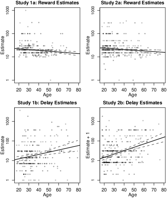
Figure 1: Relationship between age and estimates of ambiguous rewards and delays. The points have been slightly jittered to reduce overplotting. The solid lines show robust regression predictions; the dashed lines show 95% confidence limits. For Study 2b, the y-axis shows Estimate+1 because of the presence of a zero response in the dataset. Note that the slope in the top two panels is somewhat flattened by the scaling of the y-axis, which has to accommodate a handful of estimates that are below the value of the immediate reward.

---

2.2.2  Choice Behaviour

The proportions of people choosing the delayed option in each study are shown in Table 2 and suggest that, overall, the majority of participants in all studies preferred the larger-later option. Figure 2 plots the proportion of people who chose to wait in each experiment as a function of whether they under- or over-estimated the missing value.

---

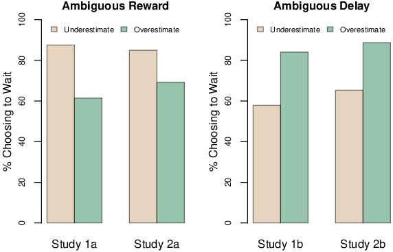
Figure 2: Proportion of participants choosing the delayed option when the delayed reward was ambiguous (Studies 1a and 2a) and when the delay was ambiguous (Studies 1b and 2b), grouped by whether the participant under- or over-estimated the missing attribute.

---

The plot suggests that people who overestimated the delayed reward were less likely to choose the delayed option than those who underestimated it; likewise, those who underestimated the delay found the future option less attractive than those who overestimated the waiting time. Table 4 shows the results of robust logistic regression of choices on age, gender, and (log-transformed) estimates of the missing reward or missing delay. There is little indication that choices are associated with the demographic variables; however, as expected, the willingness to choose the delayed option is positively associated with the estimated delay and negatively associated with the estimated reward.

---

Table 4: Results of robust logistic regression of choices on age, gender, and estimates of the ambiguous attributes, for Studies 1a–2b.

Ambiguous Reward
	Study 1a					Study 2a
	B	LL	UL	p		B	LL	UL	p
Intercept	5.414	3.558	7.270	<.001		3.515	2.376	4.654	<.001
Estimate	−3.369	−4.718	−2.019	<.001		−1.747	−2.514	−0.981	<.001
	Tjur’s R2= .143					Tjur’s R2= 0.073
Intercept	0.848	0.583	1.114	<.001		1.051	0.802	1.299	<.001
Age	0.007	−0.018	0.031	.603		−0.004	−0.023	0.014	.652
	Tjur’s R2= .001					Tjur’s R2= .001
Intercept	0.859	0.592	1.127	<.001		1.031	0.777	1.286	<.001
Gender	−0.288	−0.824	0.248	.292		0.160	−0.352	0.673	.540
	Tjur’s R2= .004					Tjur’s R2= .001
Intercept	5.586	3.651	7.521	<.001		3.585	2.416	4.755	<.001
Age	−0.008	−0.035	0.019	.559		−0.011	−0.031	0.009	.273
Gender	−0.185	−0.775	0.404	.538		0.143	−0.396	0.682	.603
Estimate	−3.506	−4.918	−2.095	<.001		−1.806	−2.592	−1.019	<.001
	Tjur’s R2= .147					Tjur’s R2= .077
Ambiguous Delay
	Study 1b					Study 2b
	B	LL	UL	p		B	LL	UL	p
Intercept	-0.805	−1.474	−0.135	.019		−0.517	−1.288	0.254	.189
Estimate	1.360	0.802	1.917	<.001		1.362	0.748	1.975	<.001
	Tjur’s R2= .115					Tjur’s R2= .081
Intercept	0.819	0.554	1.085	<.001		1.260	0.994	1.527	<.001
Age	0.007	−0.014	0.028	.522		0.008	−0.013	0.029	.449
	Tjur’s R2= .002					Tjur’s R2= .002
Intercept	0.828	0.561	1.094	<.001		1.329	1.040	1.618	<.001
Gender	−0.340	−0.876	0.196	.214		−0.463	−1.052	0.127	.124
	Tjur’s R2= .006					Tjur’s R2= .008
Intercept	−0.801	−1.488	−0.114	.022		−0.578	−1.393	0.236	.164
Age	−0.004	−0.027	0.020	.764		−0.012	−0.035	0.012	.344
Gender	−0.147	−0.731	0.438	.623		−0.171	−0.795	0.452	.590
Estimate	1.358	0.791	1.926	<.001		1.422	0.786	2.058	<.001
	Tjur’s R2= .117					Tjur’s R2= .085
Note: B = regression coefficient; LL and UL = lower and upper 95% confidence limits.

---

2.3  Discussion

Overall, the results were consistent with our hypotheses: as in previous work, greater age (at least among the population sampled here) was associated with more pessimistic expectations about future options; and the extent to which people expected the future reward to be large or the delay short was negatively associated with their willingness to wait for the actual delayed option. The latter results support the idea that, when faced with intertemporal choice under uncertainty, people’s explicit inferences about the likely value of the ambiguous attribute shape their preferences when that ambiguity is subsequently resolved. They may also support the proposition that intertemporal preferences depend, in part, on the interplay between actual and expected trade-offs between money and time. More broadly, these results accord with studies demonstrating the importance of inference to decision-making (e.g., Hohle & Teigen, 2018; Leong et al., 2017; Matthews et al., 2016).

3  Studies 3a, 3b, and 3c

Study 3 investigated the delay-reward heuristic when the value of the ambiguous attribute remained uncertain at the point of choice. In Studies 1 and 2 of the current paper, participants were told a fixed "true" value for the missing delay or reward, which might (but almost always did not) coincide with their own estimate. In Skylark et al. (2020), participants were told that their own estimates of the missing attributes were correct prior to choosing between the immediate and delayed rewards. In Study 3, we did not tell people the true value of the missing attribute: the delayed option remained ambiguous. This meant that we could also examine the effect of response order on estimates and choices – that is, were estimates and choices affected by whether people made a choice prior to estimating, or vice-versa?

We first ran a pre-registered experiment in which participants were randomly assigned to a task in which the future reward was ambiguous (Study 3a) or the delay until that reward was ambiguous (Study 3b) (the pre-registration is available from https://aspredicted.org/md6rc.pdf. Unlike Studies 1 and 2, the delay until the future reward was specified in days, avoiding the need to have participants in the delay-estimation task select a unit. The potential advantages of this are: (1) it matches the approach in some widely-used measures of delay discounting (e.g., Kirby et al., 1999), (2) it might reduce the potential for demand effects resulting from the experimenter’s selection of a set of units from which to choose (e.g., the inclusion of "years" as a possible unit might engender larger estimates than would arise spontaneously), and (3) it might lead to more precise statements of the estimated/inferred delay. However, the results from this study were somewhat surprising and we suspected that the requirement to estimate a delay in days might artificially compress the range of estimates produced – and thereby limit the potential for those estimates to predict other variables. We therefore ran a second pre-registered experiment, Study 3c, after completing Studies 3a and 3b; Study 3c was identical to Study 3b except that, like Studies 1b and 2b, the delay estimates allowed the participant to select their own temporal unit (the pre-registration is available here: https://aspredicted.org/sp5ji.pdf). Quoting from the pre-registration document for Studies 3a and 3b, the hypotheses and research questions were:

H1a. Estimated rewards will be larger for larger stated delays.

H1b. Estimated delays will be larger for larger stated rewards.

H2a. Estimated rewards will be negatively associated with participant age.

H2b. Estimated delays will be positively associated with participant age.

H3a. The tendency to choose the delayed option will be positively associated with stated future rewards.

H3b. The tendency to choose the delayed option will be positively associated with estimated future rewards.

H3c. The tendency to choose the delayed option will be negatively associated with stated future delays.

H3d. The tendency to choose the delayed option will be negatively associated with estimated future delays.

We also wish to ask: Are estimates and choices, and the effects of stated values on estimates and choices, influenced by response order (estimates before choices or vice-versa)? Are estimates affected by gender? And are choices affected by gender and/or age?

In light of the results from Studies 3a and 3b, the pre-registration for Study 3c put more emphasis on questions than hypotheses:

H1. Estimated delays will be larger for larger stated rewards.

H2. Estimated delays will be positively associated with participant age.

We also wish to ask whether estimates are affected by gender, and whether the tendency to choose the delayed option is associated with age and/or gender. More importantly, we wish to ask whether the tendency to choose the delayed option is associated with the stated value of the future reward, the estimated delay, the response order (estimates before choices or vice-versa), and the interactions between these variables.

3.1  Methods

3.1.1  Design and Procedure

Each of the studies employed a 2x2 fully between-subjects design. The first factor was the value of the unambiguous attribute of the future option; this stated value was either small (4 days when the reward was ambiguous; £13 when the delay was ambiguous) or large (122 days when the reward was ambiguous, £38 when the delay was ambiguous; all of these values were taken from Skylark et al., 2020). The second factor was the order of the tasks: estimate the ambiguous attribute then choose, or choose then estimate. Participants were randomly assigned to a cell of the design. Studies 3a and 3b were run in parallel with random assignment to study.

The procedure was identical to Studies 2a and 2b, except that (1) responses were required for all questions; (2) all delays were stated in days; thus, in Study 3a the ambiguous option was described as "Receive £X in [4 days/122 days]" and in Study 3b it was described as "Option B: Receive [£13/£38] in X day(s)". Participants in the estimation-before-choice condition entered their estimate of the missing attribute and clicked continue; at this point, the text describing the scenario and the two options remained on-screen, but the request for the estimate and the participant’s response disappeared and were replaced by the choice question ("Which would you choose?" with radio buttons for Option A and Option B). For the choices-then-estimates order, the procedure was very similar but the participant’s choice was replaced by the question asking them to estimate the missing attribute.

The second pre-registered experiment (Study 3c) was identical to Study 3b except that the delay-estimation task required participants to select a temporal unit (Day(s), Week(s), Month(s), Year(s)), just as in Studies 1b and 2b.

3.1.2  Participants

The final samples comprised 426 people who completed Study 3a, 434 people in Study 3b, and 428 in Study 3c.

3.2  Results

These studies had pre-registered analysis plans. However, during the process of analysing and interpreting the findings, we came to believe that deeper understanding of the estimation and choice data would come from alternative approaches. Briefly, problems with the pre-registered approaches were: (i) We did not specify bivariate analyses to examine the overall relationship between estimates, choices, and the other variables; (ii) In Studies 3a and 3b, we planned to use raw stated values and log-transformed estimates, rather than mean centring/effect coding these variables; thus, the "main effects" of variables involved in interactions with these predictors were being tested when, for example, the future reward was £0, which does not make much sense given that the immediate reward was £10; (iii) In Studies 3a and 3b, our pre-registered model of choices ignored the possibility that estimate and stated values might interact (i.e., that the effect of rewards might depend on delays and vice versa) or that this interaction might be modulated by whether estimates were made before or after choices; (iv) We did not include choices, or the interaction between choices and other variables, as a predictor of estimates. However, as we looked at the data and the effects of order on people’s responses (see below), we realised that this pre-registered approach reflected our implicit view of estimates as primary – i.e., as the cause of choices. But given that some participants make their choices before giving their estimate, it arguably makes as much sense to regard estimates as a consequence of choices; (v) Although we thought it would make sense to combine the data from the "days" and "own units" tasks (i.e., Studies 3b and 3c), and to test whether the temporal unit moderates other effects, we did not pre-register a plan to do so.

We therefore report the results of the pre-registered analyses in Appendix C and focus here on a broader set of exploratory analyses that we think give better insight into our participants’ estimation and choice performance. (The pattern of results for the predictors included in the pre-registered regression analyses are typically the same in the more complex exploratory models reported here.) Of course, all of these results should be treated with caution: there may be overfitting and false positives (especially given the number of predictors involved), and the power to detect some of the higher-order interactions may be low.

Throughout what follows, estimates were log-transformed and mean-centred, age was mean centred, gender was coded as −0.5 for males, +0.5 for females, and 0 for other/prefer not to say, stated value was coded −0.5 for the small value, +0.5 for the large value, and response order was coded -0.5 for choices before estimates, +0.5 for estimates before choices; choice was coded 0 for immediate and 1 for delayed option, and when choice was a predictor it was mean-centred. For the analysis of the data from the ambiguous-delay tasks, Study was coded 0 for Study 3b ("Days") and 1 for Study 3c ("Own Units") and then mean centred.

3.2.1  Descriptive statistics and simple bivariate analyses

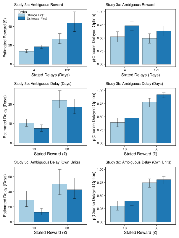
Figure 3 shows the mean estimates of the ambiguous attributes and the proportions of people who chose the delayed option in each condition for each study; the error bars show 95% confidence intervals, calculated separately for each data point (i.e., not using a pooled error term). Table 5 reports exploratory analyses examining the associations between estimates, choices, and other variables. The figure and table indicate several results. First, gender was not meaningfully associated with the estimates or choices in any of the 3 studies, but age is consistently associated with greater pessimism about the ambiguous future option: Older participants produced smaller reward estimates and longer delay estimates than did younger people. Second, larger stated delays correspond to larger estimated rewards, and larger rewards are associated with longer estimated delays – consistent with the use of a "delay-reward heuristic" when making estimates. Third, the inter-relations between stated values, estimates of missing values, and choices, are not straightforward and vary across the 3 studies; this is probably because the variables are confounded (e.g., longer stated delays are expected to make the delayed option less attractive, but also to increase the estimated reward, making the delayed option more attractive). Fourth, both estimates and choices are affected by the response order: when people make estimates before choosing, their estimates of the missing values are more optimistic (i.e., they infer larger rewards and shorter delays) and they are more likely to choose the delayed option, than when they choose before making an explicit estimate of the missing value.

Order effects imply that the act of choice can affect estimates, and hence that any attempt to understand the association between estimates and choices might just as reasonably predict choices from estimates as estimates form choices. Correspondingly, the regression analyses reported below probe both types of model using a full set of predictors.

---

Figure 3: Geometric mean estimates and choice proportions in Studies 3a-3c. The left panels show the mean estimates for each stated value as a function of whether the estimates were made before choices, or choices before estimates (error bars show 95% confidence intervals). The right panels show the proportion of participants choosing the delayed option (error bars show 95% Wilson confidence intervals).

---

---

Table 5: Bivariate relations between estimates, choices, and other variables.

	Study 3a: Ambiguous Reward
	Predicting Estimates						Predicting Choices
	B	LL	UL	Radj2	p		B	LL	UL	R2	p
Age	−0.004	−0.007	−0.002	.028	<.001		−0.017	−0.031	−0.002	.012	.024
Gender	0.052	−0.013	0.117	.003	.120		−0.133	−0.53	0.265	.001	.512
Delay	0.242	0.179	0.305	.124	<.001		−0.317	−0.706	0.072	.006	.110
Order	0.123	0.060	0.186	.032	<.001		0.764	0.369	1.159	.034	<.001
Choice	0.204	0.142	0.266	.089	<.001
Estimate							2.364	1.577	3.152	.106	<.001
	Study 3b: Ambiguous Delay – Days
	Predicting Estimates						Predicting Choices
	B	LL	UL	Radj2	p		B	LL	UL	R2	p
Age	0.009	0.006	0.012	.057	<.001		−0.002	−0.017	0.013	.000	.770
Gender	−0.027	−0.119	0.066	−.002	.574		−0.208	−0.613	0.198	.002	.316
Reward	0.380	0.297	0.462	.161	<.001		2.102	1.626	2.577	.202	<.001
Order	−0.069	−0.159	0.021	.003	.135		0.693	0.292	1.094	.027	<.001
Choice	0.198	0.105	0.291	.037	<.001
Estimate							0.834	0.393	1.275	.033	<.001
	Study 3c: Ambiguous Delay – Own Units
	Predicting Estimates						Predicting Choices
	B	LL	UL	Radj2	p		B	LL	UL	R2	p
Age	0.014	0.008	0.02	.050	<.001		−0.027	−0.043	−0.011	.025	.001
Gender	−0.055	−0.209	0.098	−.001	.481		−0.293	−0.685	0.100	.005	.145
Reward	0.407	0.264	0.55	.069	<.001		1.857	1.429	2.285	.183	<.001
Order	−0.188	−0.338	−0.039	.013	.014		0.322	−0.062	0.705	.006	.100
Choice	−0.051	−0.203	0.101	−.001	.511
Estimate							−0.129	−0.374	0.116	.003	.302
Note: The associations between estimates and other variables were assessed with robust linear regression; the associations between choices and other variables were assessed with robust logistic regression. The intercepts are not shown, for brevity. For the choice models, R2 is Tjur’s R2. B = regression coefficient; LL and UL = lower and upper 95% confidence limits.

---

3.2.2  Regression analyses for Study 3a (ambiguous rewards)

We regressed estimates on age, gender, stated delay, response order, choice, and the two- and three-way interactions between stated delay, order, and choice. Likewise, we regressed choices on age, gender, stated delay, response order, estimate, and two- and three-way interactions between stated delay, order, and estimate. All analyses used robust regressions, as described for Studies 1 and 2. The regression results are shown in Table 6; to facilitate interpretation of the results, Figure 4 shows the mean estimates for each condition organized by whether the participant selected the immediate or delayed option, and Figure 5 shows the proportion of participants choosing the delayed option, with the data grouped by whether the participant’s estimate of the missing attribute was low (equal to or less than the median estimate) or high (greater than the median). In these figures, like in Figure 3, the error bars show 95% confidence intervals calculated separately for each data point, and are intended to give some indication of the variation in the data rather than to provide the basis for inference about differences between conditions.

---

Table 6: Robust regression models for estimates and choices from Study 3a (Ambiguous Rewards).

	Predicting Estimates					Predicting Choices
	B	LL	UL	p		B	LL	UL	p
Intercept	−0.031	−0.06	−0.002	.037		1.012	0.658	1.367	<.001
Gender	0.052	−0.005	0.109	.075		−0.241	−0.698	0.216	.301
Age	−0.004	−0.006	−0.002	<.001		−0.009	−0.026	0.008	.286
Stated Delay	0.259	0.202	0.316	<.001		−1.603	−2.307	−0.899	<.001
Order	0.101	0.044	0.158	.001		0.384	−0.322	1.091	.286
Choice	0.190	0.131	0.248	<.001
Choice*Order	−0.123	−0.240	−0.007	.039
Stated Delay*Order	0.052	−0.062	0.166	.370
Choice*Stated Delay	0.057	−0.060	0.173	.341
Choice*Stated Delay*Order	−0.151	−0.384	0.082	.206
Estimate						4.028	2.552	5.505	<.001
Estimate*Order						−1.935	−4.893	1.023	.200
Stated Delay*Order						0.294	−1.116	1.704	.683
Estimate*Stated Delay						−5.153	−8.101	−2.204	<.001
Estimate*Stated Delay*Order						0.507	−5.403	6.418	.866
	R2 = .290, Radj2 = .274					Tjur’s R2 = .191
Note: B = regression coefficient; LL and UL = lower and upper 95% confidence limits.

---

---

Figure 4: Geometric mean estimates in Studies 3a–3c, organized by task order and whether the participant chose the immediate or delayed option. Error bars show 95% confidence intervals.

---

---

Figure 5: Choice proportions in Studies 3a–3c, organized by task order and whether the participant’s estimate of the missing attribute was low (equal to or below the median) or high (greater than the median). Error bars show 95% Wilson confidence intervals.

---

Predicting estimates. Estimated rewards were larger when participants were older, the stated delay was longer, the participant chose the delayed option, and when estimates were made before choices. The latter two effects were qualified by an interaction: the association between estimated reward and choosing the delayed option was stronger when choices were made before estimates. (This interaction is visible in the top row of Figure 4, where the difference in height between the dark and pale green bars is greater for the "Choice First" condition than for the "Estimate First" condition. The figure also suggests that the association between estimates and choices is stronger when the stated delay was 122 days than when it was only 4 days, but this interaction does not emerge in the regression analysis.)

Predicting choices. The tendency to wait was greater for shorter stated delays and for larger estimated rewards; in addition, the effects of stated delay and estimated reward interacted such that the effect of inferred reward was less positive when the stated delay was large. (The interaction can be seen in the top row of Figure 5, where the difference between the dark and pale purple bars is greater in the left-hand panel than in the right-hand panel.)

3.2.3  Regression analyses for Studies 3b and 3c (ambiguous delays)

We pooled the data from the two ambiguous-delays tasks (Study 3b, where estimates had to be made in days, and Study 3c, where people selected their own temporal unit) and modelled the estimates and choices using the same models as for the preceding study except that study and its interaction with all other terms in the model were also included as predictors. The results are shown in Table 8; for information, the results from Studies 3b and 3c considered separately are shown in Table 9.

Predicting estimates. Estimated delays were longer when the participants were older and when the stated reward was larger. These effects were weakened when estimates were made in days (Study 3b, middle row of Figure 4) rather than self-chosen temporal units (Study 3c, bottom row of Figure 4), and the specification of days as the unit also produced an overall reduction in the estimated delay (note the difference in y-axis scales for the middle and bottom rows of Figure 4; the scales are also somewhat stretched by the wide confidence intervals caused by the presence of a handful of large values in the £38 condition). The temporal unit also moderated the effect of choice on estimated delay: when estimates had to be made in days, there was no reliable association between estimates and choices; when estimates were made in self-selected units, people who chose to wait produced smaller estimates than those who chose the immediate option. Taken together, these results suggest that the specification of days as the temporal unit compressed the estimated delays, and that this range restriction weakened the potential for estimates to correlate with other variables. (Further support for this idea comes from consideration of the range of the estimates in the two studies: when the delays had to be estimated in days, responses were between 1 and 1000 days, with an inter-quartile range of 7 to 30 days; when specified in self-chosen units, estimates ranged from 0.01 days to 7300 days, with an IQR of 7 to 91.25 days).

There were also effects involving response order: estimated delays were longer when choices were made first, and there was a two-way interaction between order and choice, and a three-way interaction between order, choice, and stated value. Decomposing the three-way interaction (by dummy-coding response order and stated reward), the only reliable association between choices and estimates arose when choices were made first and the stated reward was large – in which case, preference for the delayed option was associated with shorter estimated delays. (This effect can be seen in the centre-right and bottom-right panels of Figure 4.)

Predicting choices. The tendency to take the delayed option was positively associated with the stated reward and negatively associated with age. The willingness to wait was also greater when the delay was estimated in days (Study 3b, middle row of Figure 5 rather than self-chosen units (Study 3c, bottom row of Figure 5) and when estimates preceded choices – but these two effects were qualified by an interaction: when choices preceded estimates, the own-unit and "days" versions of the task were similar; when estimates preceded choices, people were more likely to wait when estimates had to be made in days. (It is tempting to think that this is because the "days" unit engenders shorter estimated waiting times, but recall that this analysis controls for the estimates themselves.) The effect of order makes some sense: when choices come first, whether the missing delay is expressed as "X days" or just "X" is less likely to affect people’s decisions than when they have had to come up with an explicit estimate of the missing value.

There was no overall effect of estimated delay, but there is some indication that the effect of estimated delay was moderated by temporal units: the 95% CI for the interaction only just included 0, and the results for Study 3b (days) indicated no effect of estimates on choices whereas those for Study 3c (own units) found that people who produced larger delay estimates were less likely to choose the delayed option. (In the middle row of Figure 5, the pale purple and dark purple bars are similar; in the bottom row, the pale bars are higher than the dark ones). This pattern mirrors the results of the previous section, where estimates were the dependent variable and choice behaviour a predictor.

---

Table 7: Robust regression models for estimates and choices after pooling data from Studies 3b (Ambiguous Delays – Days) and 3c (Ambiguous Delays – Own Units).

	Predicting Estimates					Predicting Choices
	B	LL	UL	p		B	LL	UL	p
Intercept	−0.027	−0.071	0.017	.231		0.695	0.490	0.901	<.001
Gender	−0.062	−0.139	0.015	.114		−0.319	−0.653	0.016	.062
Age	0.011	0.008	0.014	<.001		−0.020	−0.033	−0.006	.004
Stated Reward	0.414	0.326	0.501	<.001		2.261	1.860	2.662	<.001
Order	−0.177	−0.263	−0.091	<.001		0.466	0.066	0.865	.022
S(tudy)	0.374	0.286	0.462	<.001		−0.528	−0.941	−0.114	.012
Stated Reward*Order	0.060	−0.113	0.232	.498		−0.084	−0.883	0.715	.837
S*Gender	−0.098	−0.251	0.056	.212		−0.306	−0.974	0.363	.370
S*Age	0.007	0.001	0.013	.025		−0.005	−0.032	0.021	.686
S*Stated Reward	0.204	0.030	0.378	.022		0.163	−0.646	0.972	.693
S*Order	−0.080	−0.252	0.093	.365		−1.003	−1.800	−0.205	.014
S*Stated Reward*Order	0.206	−0.139	0.551	.242		−1.077	−2.673	0.519	.186
Choice	−0.076	−0.168	0.016	.106
Choice*Stated Reward	−0.059	−0.242	0.123	.524
Choice*Order	0.192	0.009	0.375	.040
Choice*Stated Reward*Order	0.509	0.143	0.875	.006
S*Choice	−0.288	−0.472	−0.104	.002
S*Choice*Stated Reward	−0.118	−0.482	0.247	.527
S*Choice*Order	−0.033	−0.399	0.333	.860
S*Choice*Stated Reward*Order	0.676	−0.056	1.407	.071
Estimate						−0.141	−0.481	0.199	.418
Estimate*Stated Reward						−0.125	−0.800	0.550	.717
Estimate*Order						0.574	−0.098	1.246	.094
Estimate*Stated Reward*Order						1.072	−0.270	2.414	.118
S*Estimate						−0.672	−1.350	0.005	.052
S*Estimate*Stated Reward						−0.105	−1.450	1.239	.878
S*Estimate*Order						−1.078	−2.418	0.263	.115
S*Estimate*Stated Reward*Order						1.808	−0.869	4.485	.186
	R2 = .255, Radj2 = .239					Tjur’s R2 = .250
Note: B = regression coefficient; LL and UL = lower and upper 95% confidence limits.

---

---

Table 8: Robust regression models for estimates and choices from Study 3b (Ambiguous Delays – Days) and Study 3c (Ambiguous Delays – Own Units).

	Study 3b: Ambiguous Delay (Days)
	Predicting Estimates					Predicting Choices
	B	LL	UL	p		B	LL	UL	p
Intercept	−0.036	−0.084	0.011	.137		0.896	0.615	1.177	<.001
Gender	−0.009	−0.092	0.074	.832		−0.167	−0.645	0.311	.494
Age	0.007	0.004	0.011	<.001		−0.017	−0.035	0.002	.076
Stated Reward	0.326	0.230	0.422	<.001		2.193	1.633	2.753	<.001
Order	−0.136	−0.230	−0.041	.005		0.772	0.214	1.330	.007
Choice	0.073	−0.033	0.179	.176
Choice*Order	0.175	−0.037	0.387	.106
Stated Reward*Order	−0.022	−0.211	0.167	.820
Choice*Stated Reward	0.015	−0.197	0.226	.892
Choice*Stated Reward*Order	0.211	−0.214	0.636	.331
Estimate						0.193	−0.396	0.782	.520
Estimate*Order						1.109	−0.054	2.273	.062
Stated Reward*Order						0.421	−0.696	1.537	.460
Estimate*Stated Reward						−0.073	−1.241	1.096	.903
Estimate*Stated Reward *Order						0.174	−2.151	2.500	.883
	R2 = .224, Radj2 = .207					Tjur’s R2 = .236
	Study 3c: Ambiguous Delay (Own Units)
	Predicting Estimates					Predicting Choices
	B	LL	UL	p		B	LL	UL	p
Intercept	−0.009	−0.085	0.068	.826		0.384	0.119	0.649	.005
Gender	−0.104	−0.244	0.035	.143		−0.473	−0.939	−0.006	.047
Age	0.014	0.008	0.019	<.001		−0.022	−0.041	−0.003	.020
Stated Reward	0.499	0.347	0.650	<.001		2.312	1.791	2.833	<.001
Order	−0.246	−0.397	−0.095	.002		−0.033	−0.553	0.486	.900
Choice	−0.210	−0.366	−0.055	.008
Choice*Order	0.155	−0.153	0.464	.323
Stated Reward*Order	0.171	−0.131	0.473	.267
Choice*Stated Reward	−0.111	−0.417	0.195	.478
Choice*Stated Reward*Order	0.895	0.282	1.508	.004
Estimate						−0.479	−0.814	−0.144	.005
Estimate*Order						0.032	−0.631	0.695	.925
Stated Value*Order						−0.279	−1.319	0.761	.599
Estimate*Stated Reward						−0.178	−0.843	0.487	.600
Estimate*Stated Reward*Order						1.982	0.660	3.304	.003
	R2 = .18, Radj2 = .166					Tjur’s R2 = .253
Note: B = regression coefficient; LL and UL = lower and upper 95% confidence limits.

---

3.3  Discussion

These results were generally consistent with our hypotheses, but also indicated effects that we had not envisaged and which cast new light on the relations between inference and choice.

As expected, estimates of the ambiguous attribute (reward or delay) were positively associated with the stated attribute (delay or reward), consistent with a "delay-reward heuristic" (Skylark et al., 2020), and older participants inferred longer delays and smaller rewards than did younger participants. When we started these experiments, we expected that both stated and estimated rewards and delays would reliably predict people’s preference for the delayed option. This expectation was met for rewards: both stated and estimated rewards were positively associated with the willingness to wait (the effect of estimated reward being more pronounced when the delay was shorter). However, the results for stated and estimated delays were less consistent. In the bivariate analyses, stated delays were not associated with choices in Study 3a, and estimated delays were not associated with choices in Study 3c; in Study 3b, longer estimated delays were associated with greater willingness to wait. These results are hard to interpret because they do not control for other variables. In the regression analyses, the effect of stated delay was as expected: larger values correspond to less willingness to wait, although the effect is more pronounced when the estimated reward is larger. When delays had to be estimated, the pooled analyses indicate no overall association between estimates and choices but the results differ between the studies: when estimates were in self-selected units, there was an overall tendency to be less willing to wait as the estimated delay increased, but there was no such effect when estimates had to be made in days – which we attribute to compression of the delay estimates in this version of the task.

Perhaps more importantly, Studies 3a–3c found that inferences, choices, and their associations depend on task demands – notably, whether delay estimates had to be made in days or in a self-selected temporal unit, and whether estimates were made explicit before or after choices. We explore the implications of these findings in the General Discussion.

4  General Discussion

We replicated the finding of a delay-reward heuristic reported by Skylark et al. (2020): when future rewards were ambiguous, people’s estimates of the value of the reward were positively correlated with the stated length of the delay; when delays were ambiguous, they were inferred to be longer when the reward was larger. This result is perhaps unsurprising, but as discussed in Skylark et al., neither is it a foregone conclusion, and it is not accommodated by conventional economic accounts of intertemporal choice. We assume that the delay-reward heuristic reflects learned experience about the environmental trade-offs between money and time, in keeping with the broad view of human decision making as ecologically adapted, tuned to the statistical properties of the recent past (e.g., McGuire & Kable, 2012, 2013; Pleskac & Hertwig, 2014; Rigoli et al., 2017). However, this assumption remains to be tested by manipulating the learning environment and examining the consequences of different delay-reward contingencies for inference and preference (cf. Leuker et al., 2018, 2019a, 2019b).

The main contribution of our work is that it clarifies the role of the delay-reward heuristic in choice behaviour. Studies 1 and 2 suggest that, when people explicitly estimate the value of an ambiguous attribute, their estimate shapes their preference when the ambiguity is resolved: the more pleasantly surprising (or less unpleasantly surprising) the future option was, the more likely people were to choose it. The implication is that differences in people’s expectations underlie differences in their preferences. One obvious question is whether the kind of expectation effect found in Studies 1 and 2 might be at work in "standard" intertemporal choice tasks, where all options are fully explicated from the start. For example, when offered a choice between £10 now and £20 in 3 months, is preference for the delayed option shaped by the decision-maker’s latent belief about the growth in reward typically associated with a 3-month wait? When we conducted Studies 1 and 2, we thought that finding an expectation effect in those studies would support this broader view of the role of latent expectations in intertemporal choice. However, Studies 3a–3c urge caution about such a conclusion.

In those studies, estimates and choices were both dependent on which was made first. But if the estimates of ambiguous attributes are affected by whether or not a choice has been made, we cannot take the stated estimate as a stable latent belief that shapes preference. Likewise, we found some evidence that choices and response order interact when predicting estimates, suggesting that the nature of the association between inference and preference depends on whether choices are made before or after estimates (although these interactions are weak and exploratory, and so must be treated with caution).

What underlies the order effects? When people chose before estimating, they were less likely to select the delayed option than when they estimated before choosing – that is, when choices came first, there was greater ambiguity aversion. A straightforward explanation is that, when people make an explicit estimate before choosing, the estimate is treated as if it were correct (or as the most likely value in a distribution of plausible values); the act of explicit estimation reduces perceived ambiguity rendering the delayed option more attractive, whereas those who choose first do so on the basis of the presence of ambiguity, without forming a clear idea of what the ambiguous attribute value might be. But if the preferences of people who chose before estimating are often made without inferring the missing value, why are their subsequent estimates correlated with their preference? It seems plausible that the choice itself is used as a source of information about the missing value (e.g., "I chose Option A, so Option B must be undesirable…"; cf Ariely & Norton, 2008; Brehm, 1956; Johansson et al., 2013). Such an inference is arguably sensible because, in general, our choices reflect information about attribute values – even if, in the scenario studied here, they do not.

Of course, it is unlikely that these two pathways are "process pure": some people may implicitly infer the missing attribute even when first asked for a choice, and some people may choose based on an aversion to ambiguity even if they have just made an explicit estimate of the missing value. Moreover, the foregoing speculation is tempered by a recent study of the risk-reward heuristic. Specifically, the supplementary material of Pleskac et al. (in press) examines order effects in a version of the probability-estimation task employed by Pleskac and Hertwig (2014) and reports a pattern of results that is broadly the opposite of those obtained in the present paper: the probability estimates of participants who chose whether or not to play the risky option before estimating the ambiguous probability first were, on average, higher (more optimistic) than the estimates of those who estimated before choosing. Likewise, participants who chose before estimating were more likely to decide to play than those who estimated first. Pleskac and colleagues note that “[i]t is difficult to draw strong conclusions about the order effect as the study was not designed to examine this effect” (p. 3), and the analysis strategy used in their work is similar to that originally planned for the current Studies 3a and 3b – which, as discussed above, may not give the full picture when order effects are present. Nonetheless, the differences from the current results are intriguing and merit further investigation. In any case, the overall pattern to emerge from both sets of studies is that, as a general principle, there are distinct routes to inference and preference depending on the order in which they are elicited.

Two further results deserve brief discussion: older participants were more pessimistic than younger ones about ambiguous rewards and delays, and people’s estimates of ambiguous delays were smaller when they had to be stated in days than when people selected their own temporal unit. The age effect was first reported and discussed by Skylark et al. (2020) and could reflect differences in general dispositional optimism – although studies of age effects on optimism provide, at best, very mixed support for this view (e.g., Durbin et al., 2019; Glaesmer et al., 2012; Schwaba et al., 2019). Alternatively, the age effect might be due to different pre-experiment experiences (i.e., older people having more experience of relatively gradual growth in rewards over time – for example, by studying conventional stock market movements rather than highly volatile cryptocurrency exchange rates). One interesting question is whether the observed age difference extends to the loss domain. An optimism account predicts that, confronted with ambiguity, older people will expect larger losses and shorter timescales than younger people. The ecological-experience argument is more flexible. For example, if the present results arise because younger people have experienced more dynamic environments, they might also expect steeper losses over shorter times. In any case, it is also notable that, although we found reliable associations between age and estimates of ambiguous attributes, age was not consistently associated with choice behaviour. This is rather puzzling given the associations between estimates and choices. One possibility is that the link between estimates and choices is age-dependent (i.e., that age and estimates interact). Given the number and complexity of the analyses already reported here we have not explored this possibility, but it might be worth investigating in future.

Our finding that specifying the temporal unit to be "days" led participants to produce delay estimates that were smaller and with a narrower range is consistent with accounts that emphasize conversational pragmatics (i.e., if a value is estimated in small units, it is probably small; see e.g., Zhang & Schwarz, 2012), and fits with a body of work showing that attitudes to temporally distant outcomes depends on the units in which the delay is expressed (e.g., Pandelaere et al., 2011). Some studies of intertemporal choice specify delays in nested units (days, weeks, months, years; e.g., Matthews, 2012); others put all delays in days, even when the delay is several months or years (e.g., Kirby et al., 1999). Our results suggest that the latter might lead to the delays being perceived as especially lengthy, with corresponding diminution of people’s willingness to wait. There is evidence for such an effect (Monga & Bagchi, 2012; Siddiqui et al., 2017), although it does not always emerge (LeBoeuf, 2006; Read et al., 2005) and seems to depend on the nature of the delayed outcome and the participant’s "mind set" (Monga & Bagchi, 2012; Siddiqui et al., 2017).

An important limitation of this work is that we probed inferences about the delays and rewards that participants believe they will encounter in Psychology experiments. We chose this framing because most theorizing about the psychology of intertemporal choice is based upon such experiments, so it is important to understand the role of prior beliefs and inferences in shaping preferences in this context. However, the extent to which results from this context generalize to other scenarios remains an important open question. In particular, our framing raises the possibility that people’s inferences are based on beliefs about how psychologists construct stimuli rather than past experience with delay-reward trade-offs. Of course, in some respects it is the beliefs, rather than the basis for the beliefs, that matters most. Nonetheless, in future it will be important to explore the generality of the current findings.

5  Conclusions

The studies suggest that, when confronted with an intertemporal choice for which the "larger-later" option is ambiguous, people make explicit estimates of the uncertain values by considering the magnitude of the reward or delay. These explicit estimates in turn predict preference for the delayed option, both when that option remains ambiguous and when the ambiguity is resolved. However, we cannot conclude that people routinely deal with ambiguity by inferring the missing information, because their choices and estimates are different if they make the choice before being asked for an explicit estimate of the missing value. We suggest that, when people form an explicit estimate prior to choice, the estimate is treated as a reference point (when the true value is revealed), or as if it were accurate (when the ambiguity is unresolved) – and factors that affect the nature of the estimate, such as specifying units in which it must be made, therefore in turn affect preferences. When people choose before estimating, we suggest that there is a tendency to avoid the ambiguous option purely because it is ambiguous, and that this preference then shapes subsequent explicit estimates of the likely value of the ambiguous attribute. It seems that both preferences and inferences are "constructed" rather than "revealed" (e.g., Skylark, 2018; Slovic, 1995), such that the role of the delay-reward heuristic in choice behaviour depends on the specific conditions under which people are asked to choose.

6  References

Appendix A. Participant Sampling

6.1  Study 1

We requested participants aged 19–100, using a desktop computer, resident in the US with an approval rate of at least 95% who had not taken part in similar previous studies. We requested 550 participants for a payment of £0.40. 550 got to the end of the survey; of these, 9 failed to answer all of the questions and were excluded. A further 20 were excluded as possible duplicates (because their ip or Prolific ID occurred earlier in the data file or in a previous study, or because they self-reported past participation in the question at the end of the survey) and three participants were excluded because they entered responses that were not a single numeric value.

6.2  Study 2

We followed our pre-registered sampling plan except that, as noted, a minor error meant that participants could skip the choice question; 1 participant did so and was excluded. We requested 660 people (there was an initial glitch wherein we requested people from the US but the survey was set up to block people from outside the UK, so none of the people who tried to take the survey were allowed in. We fixed this and then proceeded with our sampling plan.) Participant requirements were as for Study 1, except that: the minimum permitted age was 18; participants had to be resident in the UK (and the survey software screened out people from outside the UK), rather than US; approval rate for past studies had to be at least 98%; and participants had to have English as their first language. Participants were paid £0.30. 661 people completed the study and answered all questions. 11 of these were excluded as possible duplicates. Of the remaining participants, 3 monetary estimates and 7 delay estimates did not conform to the pre-registered inclusion criteria (a single numeric value greater than or equal to zero) and were excluded.

6.3  Study 3

Eligibility criteria and payment were as for Study 2. For Studies 3a and 3b we requested 880 people from Prolific; a total of 883 completed the survey and were paid. Of these, 23 were marked for exclusion on the basis of self-reported past participation or id/ip duplication; there were no ineligible responses. For Study 3c: as per the pre-registration, we requested 440 people. However, in an unexpected eventuality, one person who completed the survey entered "1980" for the age question. We remunerated this person but decided to exclude them from the data set and requested a replacement. Aside from this individual, Prolific returned 441 people who completed the study; 13 were excluded as potential duplicates; there were no ineligible responses.

Appendix B. Correlations between Age and Gender

As described in our pre-registration documents, we computed the correlations between age and gender both with and without including people who specified their gender as "prefer not to say" or "other". As shown in Table 9, there was little indication of age-gender associations in any of the studies.

---

Table 9: Association (Pearson’s r) between age and gender in each study.

	Include PNTS/Other			Exclude PNTS/Other
	r (95% CI)	p		r (95% CI)	p
Study 1a	0.11 (−0.01, 0.23)	.072		0.11 (−0.01, 0.23)	.072
Study 1b	0.10 (−0.03, 0.22)	.122		0.10 (−0.03, 0.22)	.124
Study 2a	−0.02 (−0.13, 0.09)	.711		−0.02 (−0.13, 0.09)	.689
Study 2b	−0.09 (−0.20, 0.02)	.096		−0.09 (−0.20, 0.02)	.097
Study 3a	0.03 (−0.07, 0.12)	.558		0.03 (−0.07, 0.12)	.569
Study 3b	0.03 (−0.06, 0.12)	.524		0.03 (−0.06, 0.12)	.523
Study 3c	0.05 (−0.05, 0.14)	.319		0.05 (−0.05, 0.14)	.323

---

Appendix C: Pre-registered Analyses

For Studies 3a and 3b, the pre-registration specified that we would log-transform estimates as log10(x) (or log10(x+1) if zeroes are present) and regress them on age, gender, stated value, order, and the stated value*order interaction, and that we would conduct logistic regression of choices on age, gender, stated value, order, estimate, estimates*order and stated value*order. For Study 3c the pre-registration was the same except that we would mean-centre log-transformed estimates and code stated values as -0.5 for the smaller value, +0.5 for the larger value, and the regression model for choices would include estimate*condition and estimate*order*condition interactions.

For all pre-registered regression analyses of Studies 3a, 3b, and 3c, we specified that we would perform the analyses twice: once with standard regression and once with robust regression. The results for the robust regressions are shown in Table 10. The non-robust analyses yielded very similar results except that (i) for the choice data of Study 3b, the non-robust analysis also indicated a tendency for older participants to be less incmidruled to choose the delayed option, B = −0.018, CI = [-0.036, 0.000], p = .050), and (ii) for the estimation data for Study 3c, the non-robust analysis also found an interaction between stated reward and response order, such that the effect of stated reward was more positive when estimates preceded choices than when choices preceded estimates, B = 0.298, CI = [0.019, 0.576], p = .036.)

For Studies 3a and 3b, we also conducted exploratory analyses by re-fitting the pre-registered robust regression models using the centred coding scheme adopted for Study 3c; the results are shown in Table 11.

For Study 3c, the pre-registration also specified that we would fit a simpler model of the choice data by dropping the estimate*condition and estimate*order*condition interactions (i.e., the interactions included for this study but not for Studies 3a and 3b). This model comparison indicated that the more complex model was to be preferred, robust Wald test: χ² = 9.28, pseudo df = 2, p = .010. We conducted a similar model comparison for Studies 3a and 3b (i.e. by comparing the choice models shown in Tables 6 and 8 of the main text with those shown in Table 11). For Study 3a the complex model was superior (robust Wald test: χ² = 9.28, pseudo df = 2, p = .010); for Study 3b, the additional parameters did not significantly improve the fit, (robust Wald test: χ² = 0.05, pseudo df = 2, p = .977), consistent with the fact that none of the additional interaction terms were significant.

The effects found in these analyses are similar to those from the more comprehensive exploratory analyses reported in the main text, although the latter test (and find) effects not probed in the pre-registered analyses. For the sake of completeness, we here list the (typically minor) differences between the two sets of analyses in detail, focussing on differences in significance for terms that are common to both sets of regression models. For Study 3b (ambiguous delays, estimated in days), the effect of order on estimates misses significance in the pre-registered analysis (p = .070) but is significant in the exploratory analysis (p = .005). Similarly, the analysis of choice data from this study also indicates that the pre-registered model found a non-significant effect of response order (p = .174) but a just-significant interaction between order and estimated delays (p = .049); the exploratory analysis found an effect of order (p = .007) but the interaction missed significance (p = .062). Notwithstanding the folly of over-interpreting differences in whether p-values do or do not exceed .05, we note again that the pre-registered plan tests the order effects when the stated future reward is £0 – arguably a nonsensical value. Notably, the analysis in which the pre-registered model is fit but using effect-coding for the stated delay (Table 11), indicate a main effect of order like that reported in the main text – indicating that the null result in the pre-registered analysis arises because of the non-centred coding rather than because of the extra complexity of the exploratory model reported in the main text. Finally, when predicting the choices in the ambiguous-reward study (Study 3a), the pre-registered analysis finds an interaction between estimates and response order (p = .024) that is not detected in the exploratory analysis (p = .200); it is not clear why the additional interaction terms included in the latter should eliminate this effect.

---

Table 10: Results of Pre-Registered Robust Regression Analyses for Studies 3a and 3b.

	Study 3a: Ambiguous Reward
	Estimates					Choices
	B	LL	UL	p		B	LL	UL	p
Intercept	1.228	1.186	1.270	<.001		−2.358	−3.423	−1.294	<.001
Gender	0.044	−0.016	0.104	.153		−0.308	−0.755	0.139	.177
Age	−0.005	−0.007	−0.003	<.001		−0.009	−0.025	0.007	.263
Stated Delay	0.002	0.002	0.003	<.001		−0.007	−0.011	−0.003	<.001
Order	0.105	0.021	0.189	.015		3.056	0.937	5.176	.005
Stated Delay*Order	0.001	0.000	0.002	.313		0.000	−0.008	0.008	.987
Estimate						2.443	1.599	3.286	<.001
Estimate*Order						−1.934	−3.609	−0.260	.024
	R2 =.206, Radj2 = .196					Tjur’s R2 = .161
	Study 3b: Ambiguous Delay (Days)
	Estimates					Choices
	B	LL	UL	p		B	LL	UL	p
Intercept	0.723	0.630	0.816	<.001		−1.577	−2.227	−0.927	<.001
Gender	−0.010	−0.092	0.072	.812		−0.170	−0.646	0.306	.483
Age	0.007	0.004	0.010	<.001		−0.017	−0.036	0.002	.072
Stated Reward	0.015	0.011	0.018	<.001		0.087	0.065	0.109	<.001
Order	−0.169	−0.352	0.013	.070		−0.860	−2.100	0.381	.174
Stated Reward*Order	0.002	−0.004	0.009	.453		0.018	−0.026	0.062	.421
Estimate						0.214	−0.322	0.750	.435
Estimate*Order						1.057	0.003	2.112	.049
	R2 = .218, Radj2 = .208					Tjur’s R2 = .235
	Study 3c: Ambiguous Delay (Own Units)
	Estimates					Choices
	B	LL	UL	p		B	LL	UL	p
Intercept	−0.024	−0.093	0.046	.502		0.384	0.119	0.649	.005
Gender	−0.099	−0.239	0.041	.165		−0.473	−0.939	−0.006	.047
Age	0.015	0.009	0.020	<.001		−0.022	−0.041	−0.003	.020
Stated Reward	0.417	0.280	0.554	<.001		2.312	1.791	2.833	<.001
Order	−0.158	−0.295	−0.021	.024		−0.033	−0.553	0.486	.900
Stated Reward*Order	0.259	−0.015	0.533	.064		−0.279	−1.319	0.761	.599
Estimate						−0.479	−0.814	−0.144	.005
Estimate*Order						0.032	−0.631	0.695	.925
Estimate*Stated Reward						−0.178	−0.843	0.487	.600
Estimate*Stated Reward*Order						1.982	0.660	3.304	.003
	R2 = .148, Radj2 = .138					Tjur’s R2 = .253
Note: B = regression coefficient; LL and UL = lower and upper 95% confidence limits.

---

---

Table 11: Results of robust regression of pre-registered models for Studies 3a and 3b, but using mean-centred log-transformed estimates and effect-coded stated values.

	Study 3a: Ambiguous Reward
	Estimates					Choices
	B	LL	UL	p		B	LL	UL	p
Intercept	−0.033	−0.063	−0.004	.029		0.617	0.382	0.853	<.001
Gender	0.044	−0.016	0.104	.153		−0.308	−0.755	0.139	.177
Age	−0.005	−0.007	−0.003	<.001		−0.009	−0.025	0.007	.263
Stated Delay	0.247	0.188	0.306	<.001		−0.800	−1.267	−0.334	<.001
Order	0.137	0.079	0.196	<.001		0.365	−0.094	0.825	.119
Stated Delay *Order	0.061	−0.057	0.178	.313		0.008	−0.925	0.941	.987
Estimate						2.443	1.599	3.286	<.001
Estimate*Order						−1.934	−3.609	−0.260	.024
	R2 =.206, Radj2 = .196					Tjur’s R2 = .161
	Study 3b: Ambiguous Delay
	Estimates					Choices
	B	LL	UL	p		B	LL	UL	p
Intercept	−0.030	−0.071	0.011	.152		0.887	0.617	1.156	<.001
Gender	−0.010	−0.092	0.072	.812		−0.170	−0.646	0.306	.483
Age	0.007	0.004	0.010	<.001		−0.017	−0.036	0.002	.072
Stated Reward	0.367	0.285	0.448	<.001		2.179	1.629	2.730	<.001
Order	−0.106	−0.187	−0.026	.001		0.792	0.26	1.323	.004
Stated Reward *Order	0.062	−0.099	0.223	.453		0.450	−0.646	1.545	.421
Estimate						0.214	−0.322	0.750	.435
Estimate*Order						1.057	0.003	2.112	.049
	R2 = .218, Radj2 = .208					Tjur’s R2 = .235
Note: B = regression coefficient; LL and UL = lower and upper 95% confidence limits.

---

*

Department of Psychology, University of Cambridge. Email: wjm22@cam.ac.uk. https://orcid.org/0000-0002-3375-2669.

#

University of Manchester. https://orcid.org/0000-0003-2882-0310.

$

London School of Economics. https://orcid.org/0000-0002-2627-7011.

George Farmer was supported by a WellcomeInstitutional Strategic Support Fund award (204796/Z/16/Z).

Copyright: © 2021. The authors license this article under the terms of the Creative Commons Attribution 3.0 License.

This document was translated from L^AT_EX by H^EV^EA.