| Figure 1: Example of display of one trial. |
Judgment and Decision Making, Vol. 16, No. 5, September 2021, pp. 1155-1185
Multiattribute judgment: Acceptance of a new COVID-19 vaccine as a function of price, risk, and effectivenessMichael H. Birnbaum* |
Abstract:This paper illustrates how to apply the RECIPE design to evaluate multiattribute judgment, reporting an experiment in which participants judged intentions to receive a new vaccine against COVID-19. The attributes varied were Price of the vaccine, Risks of side effects as reported in trials, and Effectiveness of the vaccine in preventing COVID. The RECIPE design is a union of factorial designs in which each of three attributes is presented alone, in pairs with each of the other attributes, and in a complete factorial with all other information. Consistent with previous research with analogous judgment tasks, the additive and relative weight averaging models with constant weights could be rejected in favor of a configural weight averaging model in which the lowest-valued attribute receives additional weight. That is, people are unlikely to accept vaccination if Price is too high, Risk is too high, or Effectiveness is too low. The attribute with the greatest weight was Effectiveness, followed by Risk of side-effects, and Price carried the least weight.
Keywords: COVID, vaccine, averaging models, conjoint measurement, functional measurement, importance of variables, information integration, multi-attribute utility, recipe design, weights of attributes, configural weighting
In this study, participants were asked to judge their intentions to take a new vaccine against COVID-19, a disease that is highly infectious and which has caused many deaths. At the time of the study, there was a question whether or not people would be willing to take a new vaccine, because of disinformation campaigns against vaccination, anti-science dogma, political denials of the dangers of COVID-19, and distrust of the Trump administration in the USA, which had a reputation of promulgating false information. Polls indicated that people might not agree to accept the vaccination in sufficient numbers for a vaccine to produce "herd immunity" and thereby stop the pandemic (Hamel, et al., 2020; Dwyer, 2020).
How would decisions to accept vaccination depend on a vaccine’s Price, Risks (of side-effects), and Effectiveness? This topic provides a good illustration of how one can employ the RECIPE design to study multiattribute judgment, using new computer resources that are now available (Birnbaum, 2021).
The Recipe design is an experimental design in which it is possible to distinguish adding and averaging models, and in which weights and scale values in averaging models can be identified and estimated. The design for three factors consists of the union of each factor alone, the factorial combinations of each pair of factors with the third left out, and the complete factorial design with all three pieces of information. A factorial design with a fixed list of factors does not allow one to distinguish additive from averaging models, nor does it permit any disentanglement of weights from scale values; the fact that weights and scale values cannot be separately identified was presented as a criticism of Anderson’s (1971b, 1974) early work on functional measurement (Schonemann, Cafferty & Rotton, 1973). However, this criticism did not apply to methods for weight estimation used by Anderson (1967) or Birnbaum (1973), and it was addressed and refuted by Norman (1973, 1976).1 Luce (1981) presented an axiomatic comparison of the theories, noting how they differed.
The original RECIPE program was written in FORTRAN as an extension of Birnbaum’s (1973, 1976) programs used in studies of moral judgment and of intuitive numerical predictions. The Recipe design and program were developed to teach students and researchers how to compare additive and averaging models of information integration (Anderson, 1974) and how to separately estimate weights and scale values (Birnbaum, 1973, 1976; Birnbaum, Wong & Wong, 1976; Cooke & Mellers, 1998; Mellers & Cooke, 1994; Stevenson, Naylor & Busemeyer, 1990). Other computer programs have also been developed for this issue (Norman, 1976, 1977, 1979; Zalinski & Anderson, 1991; Vidotto, Massidda & Noventa, 2010). Special note should be made to the work of Norman (1973), who used maximum likelihood to estimate weights in a subset of the full Recipe design.
Because few people are still using FORTRAN, Birnbaum (2021) presented three computer programs to update and expand what was previously available. The three programs are Recipe_Wiz.htm, Recipe_sim.htm, and Recipe_fit.xlsx, which enable a user to (1) create Web pages that collect data via the Internet in a Recipe design, (2) to simulate data according to a relative weight averaging model with constant weights, and (3) to fit data to an averaging model by finding best-fit weights and scale values via the Solver in Excel, respectively. These resources, along with a paper and instructional video that describes them, are available at http://psych.fullerton.edu/mbirnbaum/recipe/.
The study in this paper was done using these new computer resources. Consistent with previous studies, evidence was found against the additive model and against the relative weight averaging model with constant weights. A new fitting program, Recipe_fit_config.xlsx, was created to allow for configural weighting. This new resource is included in a supplement to this paper, along with the data of this study.
The participants’ task was to read descriptions of hypothetical new vaccines for the COVID-19 virus, and to judge their intentions: how likely would they be to accept a new vaccine, based on its Price (P: cost in dollars), Risks (R: dangers of side-effects), and Effectiveness (E: how well the vaccine prevented COVID).
The adding model (Anderson, 1981; Birnbaum & Stegner, 1981; Stevenson, 1993), can be written for this situation as follows:
| PREijk = w0 s0 + wP pi + wR rj + wE ek (1) |
where PREijk is the theoretical response in the case where all three attributes, P, R, and E are presented, with levels i, j, and k, respectively, which have scale values of pi, rj, and ek, respectively. The weights (importance) of factors A, B, and C are wP, wR, and wE, respectively. The initial impression has a weight of w0 and a value of s0, which represents the response in the absence of information. In the additive model, weights and scale values cannot be separately identified (Birnbaum & Stegner, 1981; Schoenemann, 1973) because for any factor one could multiply the supposed weight by a constant and divide the scale values by that same constant, and the calculated predictions would be unchanged.
If we assume that the response is linearly related to the subjective impressions, and adopting ANOVA assumptions concerning error, there should be no two-way or three-way interactions in ANOVA.2
The relative-weight averaging model with constant weights (Anderson,1974; 1981; Birnbaum, 1976; Norman, 1976) can be written for this situation as follows:
| PREijk = |
| (2) |
where PREijk is the theoretical response in the case where all three attributes are presented, with levels i, j, and k, respectively, which have scale values and weights as defined above. The initial impression has a weight of w0 and a value of s0. In theory, s0, represents the value of the impression in the absence of information, and w0, represents how resistant this "prior" is to new information.
Key assumptions of these models are: (1) if an attribute is not presented, its weight is zero; (2) the weight of an attribute is independent of the number and value of attributes presented with it; (3) the scale values of attributes are independent of the number and values of the attributes presented with it. It is also assumed that the judgment function, J, which maps subjective impressions to overt responses, is linear; i.e., that the numerical coding of responses are an "interval scale" of subjective impressions (Anderson, 1974; Birnbaum, 1972, 1973, 1974).
These assumptions, along with ANOVA assumptions concerning error, imply that there should be no interactions in any of the two-way or three-way factorial designs.
Anderson (1974, 1981) argued that interactions observed in certain studies were minimal or not significant, and that his decision not to reject the null hypothesis in such cases "validated" the model, the estimated stimulus scales, and the response scale simultaneously. The empirical findings reviewed by Anderson and the logic of such "validation" arguments based on nonsignificance of interactions in ANOVA were among the controversies reviewed by Birnbaum (1982, Section F).
Empirical tests of the constant-weight averaging model in more tightly constrained studies led to evidence of interactions and other violations of the relative-weight averaging model with constant weights. Evidence of systematic violations led to configural weight theories (Birnbaum, Parducci & Gifford, 1971; Birnbaum, 1974, 1982, 2008; Birnbaum & Stegner, 1979).
New methods and critical tests were devised to test between the hypotheses that the interactions were due to a nonlinear response function between subjective impressions and over responses, and the alternative hypothesis that the impressions violate the averaging model with constant weights, as implied by configural weighting. Ordinal tests indicated that one could not explain the violations of the averaging models by means of a nonlinear response function; instead, one needed something like configural weighting (Birnbaum, 1974, 1982, 2008; Birnbaum & Sutton, 1992; Birnbaum & Jou, 1990; Birnbaum & Zimmermann, 1998).
The configural weight model differs from Equation 2 in that the weight of a given attribute is affected by the configuration of attribute values to be integrated. The range model is the simplest form of configural weight model (Birnbaum, et al., 1971; Birnbaum, 1974; Birnbaum & Stegner, 1979, 1981; Birnbaum & Zimmermann, 1998; Birnbaum, 2018). It can be interpreted as a type of transfer of attention exchange (TAX) model, in which a certain amount of relative weight is transferred from the highest valued stimulus component in a combination to the lowest or vice versa. This model can be written as follows: PRE_ijk = w_0 s_0 + w_P p_i + w_R r_j + w_E e_k / w_0 + w_P + w_R + w_E + ω|max(p_i,r_j,e_k)-min(p_i,r_j,e_k)| where ω is the configural weight transferred from the minimal scale value in the configuration of attribute values, min(pi,rj,ek), to the maximal value, max(pi,rj,ek), when ω > 0, or in the case of ω < 0, from the highest to the lowest.
In judgments of morality of a person based on the deeds they have done or the likeableness of a person based on the adjectives that describe them, it has been found that ω < 0.
When ω < 0, weight is transferred from the higher-valued information to the lower-valued information. Such configural weighting implies "risk aversion" in the evaluation of lotteries: if the lowest valued consequence in a gamble gets greater weight, people will prefer the the expected value of a gamble to the gamble, even when the utility function is linear (Birnbaum & Sutton, 1992; Birnbaum, 2008).
In evaluative judgments, in the "buyer’s" point of view, the value of ω is typically negative, but in the "seller’s" point of view, it can be positive (Birnbaum & Stegner, 1979; Birnbaum, Coffey, Mellers & Weiss, 1992; Birnbaum & Sutton, 1992; Birnbaum, et al., 2016; Birnbaum, 2018; Champagne & Stevenson, 1994). In this study, people are in the "buyer’s" point of view, because they are evaluating whether to accept the vaccine based on Price, Effectiveness, and Risk.
This study was done in Fall of 2020, before the FDA had approved a vaccine for COVID-19. Participants viewed the materials by visiting the website and completing a Web form that was created using Recipe_Wiz.htm.
Participants were informed, "COVID-19 virus is a highly contagious disease that can be deadly and can also leave lasting health problems for those who recover from it. Vaccines are currently being developed that are being offered to the public. This questionnaire asks how you would decide whether or not you would take a vaccine based on the price, the risk, and the effectiveness of new vaccines, based on the findings of clinical trials as described by the scientists who conducted the trials."
Price (P) was described as "the amount you must pay out of pocket to receive the vaccine." The 3 levels of P were Low Price: $20, Medium Price: $400, and High Price: $10,000.
Risk (R) was described as "…the danger of receiving the vaccine. All medicines and vaccines carry some side effects or risks of bad results that were not intended. The levels of risk are described by the worst outcomes that happened during testing…" There were 4 levels of R: Low Risk: 5% of the people got sore arms; Slightly Low Risk: 10% of the people got fevers and headaches for two weeks;Slightly High Risk: 5% of the people got damage to the kidneys;Very High Risk: 1% of those tested had heart attacks.
Effectiveness (E) was described as "…how well the vaccine worked to prevent COVID-19 infection in people who were exposed to the virus. The levels of effectiveness are based on the percentage of people who received the vaccine who got sick with COVID-19…" The 5 levels of E were: Very Low Effectiveness: 50% got sick; Low Effectiveness: 40% got sick; Medium Effectiveness: 30% got sick; High Effectiveness: 20% got sick; and Very High Effectiveness: 10% got sick.
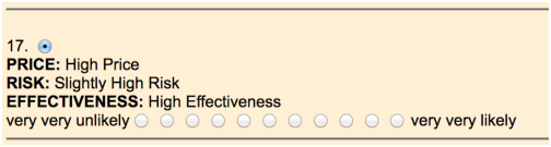
Each trial was displayed as in the format of Figure 1. Subjects were instructed, "Please make your judgments of whether or not you would be likely to try the vaccine in each case by clicking one of the buttons on the scale from very very unlikely to very very likely to try the vaccine. In some cases, some of the information is missing, but you should still do the best you can to make your decisions based on the information available."
Figure 1: Example of display of one trial.
Complete instructions, warmups, displays, and materials can be found at http://psych.fullerton.edu/mbirnbaum/recipe/vaccine_01.htm.
The Recipe design is based on three factors, designated A, B, and C, with nA, nB and nC levels. It consists of the union of the 3-way factorial design of A by B by C, denoted ABC, combined with each 2-way factorial design (with one piece of information left out), denoted AB, AC, and BC, combined with 3 designs of each piece of information presented alone: A, B, and C. There are a total of (nA+1)(nB+1)(nC+1) − 1 experimental trials ("cells") in the Recipe design. In this vaccination example, let A = Price (P), B = Risk(R), and C = Effectiveness (E).
There were 3 levels of P, 4 levels of R, and 5 levels of E, producing 119 cells (distinct experimental trials) in the design, consisting of 3 trials for the three levels of Price alone, 4 trials of Risk alone, 5 trials of Effectiveness alone, 3 by 4 = 12 PR trials of Price combined with Risk, 3 by 5 = 15 PE trials of Price by Effectiveness, 4 by 5 = 20 RE trials of Risk by Effectiveness, and 3 by 4 by 5 = 60 Price by Risk by Effectiveness (PRE) trials with all three pieces of information.
These 119 trials were intermixed and presented in random order, following a warm-up of 8 representative trials. Participants were free to work at their own paces, and all completed the task in less than one hour.
The participants were 104 college undergraduates who received partial credit (as one option) toward an assignment in Introductory Psychology at California State University, Fullerton. They were tested in Fall of 2020; data collection stopped on December 11, 2020, when the FDA provisionally authorized the first COVID-19 vaccine in the USA as an emergency measure.3
The weights and scale values of the configural weight model were estimated to minimize the sum of squared deviations between mean judgments and predictions of the model by means of an Excel workbook, Recipe_fit_config.xlsx, which uses the Solver in Excel. This Workbook, including the data of this study, are included in the supplement to this article.
Table 1 shows the best-fit parameters estimated from the averaged data. The weights have been estimated, without loss of generality, such that the sum of the weights is fixed to 1.4 According to the estimated parameters in Table 1, wE > wR > wP.
Table 1: Parameter estimates of configural-weight averaging model.
Price Risk Effectiveness Notes: w0 = 0.15, s0 = 5.84, ω = −0.21. Sum of squared deviations is 11.29; root mean squared error = 0.31.
The configural weight transfer parameter, ω = −0.21, indicating that the lowest-valued attribute is estimated to receive an additional 21% of the relative weight, transferred from the highest-valued attribute, which loses that much weight. For example, when all three pieces of information are presented, Effectiveness has a (configural) relative weight of 0.38 − 0.21 = 0.17 when its scale value is highest among the attributes, 0.38 when it is the middle value, and 0.38 + 0.21 = 0.59 when it is the lowest-valued attribute of a vaccine.
Figures 2, 3, and 4 show mean judgments of intention to accept the new vaccine in the three, two-way factorial sub-designs, in which one piece of information is missing: AB (Price by Risk), AC (Price by Effectiveness), and BC (Risk by Effectiveness), respectively. In each figure, markers represent mean judgments and lines show best-fit predictions of the configural-weight averaging model (Equation 3).
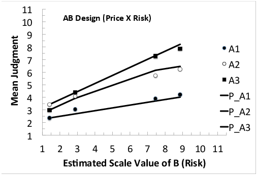
Figure 2: Mean judgments of intention to take the new vaccine in the AB design (Price by Risk), as a function of the estimated scale value of Risk (B), with separate markers and curve for each level of Price (A). A1, A2, and A3 refer to Price = $10,000, $400, and $20; the lines show the predictions of configural weight model, labeled P_A1, P_A2, and P_A3, respectively.
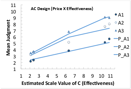
Figure 3: Mean judgments in the AC (Price by Effectiveness) design, plotted as a function of estimated scale values of C (Effectiveness), with a separate curve for each level of A (Price); markers show mean judgments and lines show best-fit predictions of the model.
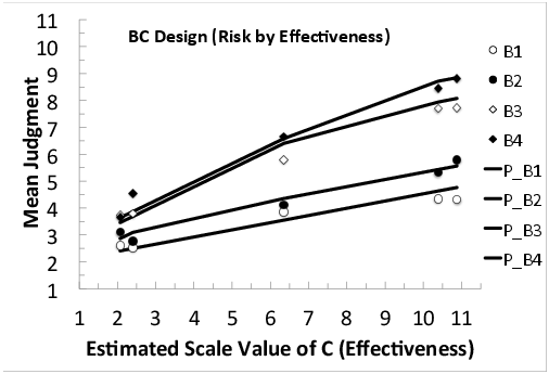
Figure 4: Mean judgments in the BC design, plotted as a function of estimated scale values of C (Effectiveness), with separate markers and curve for each level of B (Risk); markers show mean judgments and lines show best-fit predictions of the model.
In Figure 2 mean judgments are plotted against estimated scale values of Risk, with separate markers (and predicted lines) for each level of Price. Both data (markers) and predictions diverge to the right. Such divergence indicates that when either attribute is low in value, the other attribute has less effect.
Figure 3 plots mean judgments in the BC sub-design as a function of the estimated scale values of Effectiveness, with a separate curve for each level of Price. Figure 4 shows the results for the BC (Risk by Effectiveness) sub-design. In all of the two-way designs, the curves diverge to the right, and the model (lines) does a fairly good job of reproducing the data (markers).
Figures 5, 6, and 7 show the mean judgments in the ABC sub-design, which is a 3 by 4 by 5, Price by Risk by Effectiveness, factorial design. Each panel shows the Risk by Effectiveness interaction (plotted as in Figure 4) for a different level of Price, where Price (A) = $10,000, $400, and $20 in Figures 5, 6, and 7, respectively.
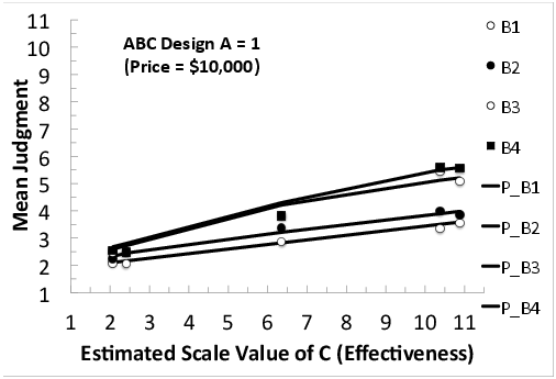
Figure 5: Mean judgments of intention to take the new vaccine in the ABC sub-design (Price by Risk by Effectiveness), plotted as a function of the estimated scale value of C (Effectiveness), with a separate curve for each level of B (Risk), where A = 1 (Price = $10,000).
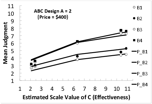
Figure 6: Mean judgments in the ABC sub-design (Price by Risk by Effectiveness), as a function of the estimated scale value of Effectiveness, with a separate curve for each level of Risk, where A = 2 (Price = $400).
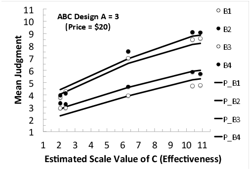
Figure 7: Mean judgments in the ABC sub-design (Price by Risk by Effectiveness), as a function of scale values of Effectiveness, with a separate curve for each level of Risk, where Price = $20.
The interactions in the data (markers) show divergence to the right in all six cases (Figures 2–7). That is, the vertical separations between the markers increase as one moves from left to right in each figure. These divergent interactions are not consistent with either the additive model or relative weight averaging model with constant weights (Equations 1 and 2). The data (markers) are fairly well-fit by the lines, showing predictions of Equation 3 (the configural weight averaging model), except perhaps in Figure 7 where the divergence in the data is even greater than predicted by the model.
In the averaging model (Equation 2), the effect of an attribute, like Price or Effectiveness, is directly proportional to the range of scale values multiplied by the weight of a factor, and it is inversely proportional to the sum of the weights of the attributes presented. The term "Zen of Weights" refers to the fact that the effects of A do not inform us clearly about the weight of A, but from the effects of A, we can instead compare the weights of B and C.5
The effects of A are defined as differences in response as the factor A is manipulated from A1 to Am. Let 1 and m refer to the levels of A that produce the lowest and highest responses for A. The indices, i, j, and k are used for the levels of A, B, and C, respectively, and a bullet ( •) is used to denote that responses have been averaged over levels of a factor.
When A is presented alone, the effect of A is defined as follows:
| Δ A = Am − A1 (3) |
where Δ A is the effect of A, defined as the difference in response to A alone, between the highest and lowest levels of A.
The effects of A in the AB design and AC designs, denoted Δ A(B) and Δ A(C), are defined respectively as follows:
| Δ A(B) = |
| m • − |
| 1 • (4) |
| Δ A(C) = |
| m • − |
| 1 • (5) |
where ABi • denotes marginal mean in the AB design for level i of A, averaged over the levels of B, and ACk • is the corresponding marginal mean for A the AC design, averaged over levels of C.
Finally, the effect of A in the ABC factorial design, denoted Δ A(BC), is given by,
| Δ A(BC) = |
| m • • − |
| 1 • • (6) |
According to the additive model, all of these effects are implied to be equal; however, according to the relative weight averaging model with constant weights (Equation 2), these effects of A are inversely related to the total weight of the information presented. That is,
| Δ A = Δ a |
| (7) |
| Δ A(B) = Δ a |
| (8) |
| Δ A(C) = Δ a |
| (9) |
| Δ A(BC) = Δ a |
| (10) |
where wA Δ a, is the same in all expressions, but the weights in the denominator are different. According to this model, the Δ A(BC) will be the smallest, and Δ A will be greatest and the other two will be in between such that if the weight of B is greater than the weight of C, then the effect of A will be less when B is presented with it than when it is paired with C.
Figure 8 plots observed and predicted marginal means (according to the configural weight model of Equation 3) as a function of the scale values for A; i.e., ai. Markers represent empirical means or marginal means. Note that the curve for A alone has the steepest slope and the curve for A(BC) has the least slope; that is Δ A > Δ A(BC). The fact that these slopes (effects) are not equal (the curves even cross) is evidence against the adding model, but consistent with either form of averaging (Equations 2 or 3).
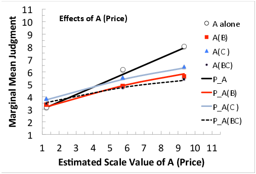
Figure 8: Effects of A (Price): Marginal mean judgments as a function of the estimated scale value of Price, with separate markers (data) and curve (predictions) for each sub-design in which A appears.
Figures 9 and 10 show effects of B and C, as in Figure 8. Figure 9, shows that the effect of B(A), Risk averaged over levels of Price (slope of the solid circles) exceeds the effect of B(C), Risk averaged over Effectiveness; therefore the weight of Effectiveness is greater than that of Price. In Figure 10, the effect of C(A) exceeds that of C(B); therefore, the weight of A (Price) is the least weighted attribute.
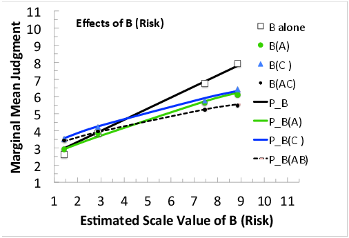
Figure 9: Effects of B (Risk): Marginal mean judgments as a function of the estimated scale value of Risk, with separate markers (data) and curve (predictions) for each sub-design including B.
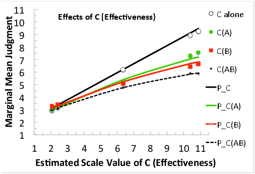
Figure 10: Effects of C (Effectiveness): Marginal mean judgments as a function of the estimated scale value of Effectiveness, with separate markers and curve for each sub-design in which C appears.
The data of each individual were analyzed separately, to assess how representative the two main conclusions are to individual participants.
Marginal means were computed for each participant in each sub-design, as in Figures 8–10, in order to test between adding and averaging models. According to the additive model, the marginal means for a variable should have the same slopes in all sub-designs, whereas averaging models imply that the effect of an attribute should be inversely related to the number (total weight) of other attributes presented with it. Of the 104 participants, 88, 86, and 87 showed greater effects of A, B, and C alone than the marginal effects of A(BC), B(AC), and C(AB), respectively; 78, 75, and 86 showed greater effects of A(B), B(A), and C(A) than in A(BC), B(AC), and C(AB), respectively; and 77, 80, and 68 showed greater effects of A(C), B(C), and C(B) than in A(BC), B(AC), and C(AB), respectively. If the additive model held, we expect half of the participants to have greater effects and half to have smaller effects. We can therefore perform a binomial sign test for each of these comparisons with p=0.5 and n=104 to test the additive model, for which the mean is 52 and standard deviation is 5.1. With 68 cases out 104 matching the prediction of averaging, z=3.14 and with 88 cases, z=7.1, so in all 9 cases, we can reject the hypothesis that the additive model describes these data (p<.001) in favor of the conclusion that significantly more than half of the sample exhibited reduced effects when all three attributes were presented compared to situations where less information was presented.
The configural weight model (Equation 3) was also fit to each participant’s data separately, in order to compare the constant weight model against the configural weight model. If a constant weight model (Equation 2) is applicable, one expects that the configural parameter would be equally likely to be less than zero (divergent interactions) or greater than zero (convergent interactions). Because the curves in Figures 2–7 should be parallel (i.e., ω = 0), by chance, an equal number should diverge or converge, respectively, producing negative or positive values of ω. It was found that 83 of the individuals were estimated to have ω < −0.01, so we can reject the hypothesis of the constant weight averaging model (z=6.08, p<0.001) in favor of the hypothesis that significantly more than half of the sample showed divergent interactions consistent with greater configural weighting on the lower-valued attribute.
The individual analyses also allow us to assess individual differences in the importance of the factors of Price, Risk, and Effectiveness. The most frequent pattern (found in 40 people) had weights in the order wE > wR > wP, the same as for the averaged data in Table 1; the second largest group (25 individuals) had weights in the order, wE > wP > wR, so a total of 65 cases had Effectiveness as the most important attribute. There were 21 who placed the most weight on Price, and 18 who put the most weight on Risk. If the weights were equal, we would expect one-third to have each attribute as most important, so the finding that 65 out of 104 had Effectiveness as most important would lead us to reject the hypothesis that all factors are equally important, in favor of the hypothesis that more than half of the sample had Effectiveness highest in weight.
The data allow us to reach two main conclusions: First, judgments of intention to accept a new vaccine do not conform to an additive model (as in Equation 1), but instead to an averaging model (as in either Equations 2 or 3). The fact that the curves in Figures 8, 9, and 10 have different slopes rules out the adding model; instead, the finding that slopes are decreased as more information is included would be compatible with either Equations 2 or 3.
Second, the data do not conform to the predictions of the relative weight averaging model with constant weights (Equation 2), which implies that the data curves in Figures 2–7 should be parallel. The fact that the data in Figures 2–7 show divergent interactions violates the implications of both Equations 1 and 2. Instead, the divergent interactions can be better fit by an averaging model with configural weights (Equation 3), in which the lower-ranked information receives greater weight and the higher-ranked values receive reduced weight (i.e., ω < 0).
The data also indicate that for the averaged data, Effectiveness was the most important factor and Price was least important in deciding whether to accept vaccination. Of course, weights and scale values in Table 1 represent average behavior of a group of college undergraduates. It would not be surprising if people with other levels of education, age, or other characteristics have different parameters.
Aside from generalizing from college students to others, one might also question the external validity of self-report studies (Levin, Louviere, Schepanski & Norman, 1983). Do stated intentions predict what people would do when presented with actual opportunities for vaccination? One of the many factors to consider is that what is considered "good" for price, effectiveness or risk would likely depend on the context of what is available in the market at a given time (Cooke & Mellers, 1998; Mellers & Cooke, 1994). Indeed, after this study was completed, it was announced that price of new COVID vaccines would not be a factor, since vaccinations would be provided by the government to everyone without charge.
Although this is the first study (to my knowledge) of vaccine acceptance using a Recipe design, I would argue that the two main findings could have been "predicted" by generalization of findings from previous research with other evaluative tasks.
First, Research with similar tasks concluded that additive models can be rejected in favor of averaging models because the effect of an attribute or source of information has been found to be inversely related to the number, reliability, validity or subjective importance of informational components with which it is combined (Anderson, 1974; 1981; Birnbaum, 1976; Birnbaum, Wong & Wong, 1976; Birnbaum & Stegner, 1979, 1981). Birnbaum and Mellers (1983, Table 2) illustrated analogies among studies that could be represented by averaging models in which weights had been manipulated by varying cue-criterion correlation, reliability, or source credibility, and where the results showed clear evidence against weighted additive models.
Second, research with evaluative judgments concluded that the relative weight averaging model with constant weights (Equation 2), can be rejected in favor of models that can imply divergent interactions. This topic is reviewed in the next section.
Table 2: Analogies among studies of judgment showing divergent interactions.
Note: See text for descriptions of these studies.
Table 2 presents a list of evaluative tasks that have reported similar, divergent interactions.6 In Table 2, deciding to accept a new vaccine is said to be similar to judging the likeableness of a person described by a set of adjectives, judging the morality of another person based on the deeds they have done, judging one’s intentions to use public bus transportation based on price and attributes representing convenience and availability of service, deciding whether an employee should be rewarded, or judging how much one should pay to buy a used car, an investment, or a risky gamble. All of these tasks involve evaluating something from the perspective of a person in the "buyer’s point of view;" i.e., deciding to purchase, receive, or to accept something or someone.
In the impression formation task, participants rate how much they would like hypothetical persons described by adjectives provided by sources who know the person. For example, how much do you think you would like a person described as "malicious" by one person and as "intelligent" by another? Anderson (1971b, 1974) had argued for a relative weight averaging model (Equation 2) to describe this impression formation task; however, well-designed studies found divergent interactions (Birnbaum, 1974; Birnbaum, Wong & Wong, 1976). If a target person is described by one source as "malicious", that person will be disliked, and the effect of a second adjective provided by another source is less than if the first source had described the target as "kind".
In Moral judgments, a person who has done one very bad deed, such as killing one’s mother without justification, is rated as "immoral" even if that person has done a number of good deeds such as donating a kidney to a child needing an organ transplant (Birnbaum, 1972, 1973; Riskey & Birnbaum, 1974). Although the more good deeds a person has done the higher the judgment, there appears to be an asymptote limiting how "moral" a person can be judged, once that person has done a very bad deed.
One can use the set-size effect to estimate weights and scale values in a differential weight averaging model (Birnbaum, 1973); according to this model, which allows weights to depend on scale value, as one adds more and more deeds of a given value, the curve should approach the scale value asymptotically and the rate of approach can be used to measure weight. The asymptote should depend only on the value of the added deeds and should be independent of the value of any initial, single deed of another value. One can also estimate differential weights by a second method, from the interactions between two deeds. The inconsistencies between asymptotes and inconsistencies between estimates of weights were taken as evidence against differential weight averaging models, which include the constant weight model of Equation 2 as a special case (Birnbaum, 1973; Riskey & Birnbaum, 1974).
Norman (1977) asked participants to rate their intentions to use a public bus based on price, distance to the bus stop, number of stops, and times of service. He reported that if one attribute had an unfavorable value, other components had a smaller effect than if that attribute had a higher value. Norman (1977) used a geometric averaging model to fit the diverging interactions among attributes he observed.7
Birnbaum and Stegner (1979) asked people to judge the most a buyer should be willing to pay for a used car, based on estimates from sources who varied in both bias and expertise. The sources were mechanics who examined the vehicle, who differed in mechanical expertise, and who were either friends of the potential buyer or seller of the car or independents. The sources provided estimates of the value of the cars. A configural weight averaging model (Equation 3 with added features) was used to represent the data. In this model, the weight of an estimate depended on the expertise of the source, and the scale value of each estimate was adjusted to reflect the bias of the source. Divergent interactions between estimates from different sources indicated that lower valued estimates received greater configural weight in determining buying prices.
In the case of judged buying prices for used cars, a very low estimate of the value of a used car by one person also appears to place an upper bound on how highly a car can be evaluated as expertise of another source who provided a high estimate is increased (Birnbaum & Stegner, 1979, Figure 10A). This phenomenon, similar to the findings for moral judgment, could be represented by a slight revision of the configural model to the form later used in the TAX model for risky gambles with different levels of probability (Birnbaum & Stegner, 1979, p. 68; Birnbaum, 2008).
Champagne and Stevenson (1994) asked people to combine information about an employee’s job performance for the purpose of rewarding good performance. They reported divergent interactions; that is, poor performance in one component of job performance tended to reduce the impact of performance on other aspects of the job in determining a reward.
Divergent interactions have also been observed in judgments of the buying prices of gambles based on the possible cash prizes of the gambles (Birnbaum & Sutton, 1992; Birnbaum, Coffey, Mellers & Weiss, 1992; Birnbaum, et al., 2016). In 50–50 gambles, if one outcome yields a low prize, judged buying prices are low and are less affected by the consequence for the other outcome than if that outcome yields a higher prize.
A classic finding in risky decision making research is "risk aversion", which refers to the finding that many people prefer a sure thing over a gamble with equal or even greater expected value. For example, most college undergraduates say they prefer $40 for sure over a fifty-fifty gamble to win either $0 or $100, which has an expected value of $50. The classic explanation is that utility of monetary gains is a negatively accelerated function of cash values. However, configural weighting provides another way to represent "risk aversion" in risky decision making, aside from nonlinear utility. Suppose the worst outcome of a 50–50 gamble gets twice the weight of the highest outcome (i.e., ω = −1/6), and suppose utility of money is linear for pocket cash: it follows that a 50–50 gamble to win $0 or $100 is worth only $33 (Birnbaum, 2008).
Birnbaum and Zimmermann (1998) found similar divergent interactions for buying prices of investments based on information from advisors, who predicted future values of the investments.
In summary, studies in Table 2 reported divergent interactions like those found here for analogous evaluative tasks. These interactions are consistent with configural weighting, as in Equation 3, if ω < 0. However, interactions might also be produced by Equation 2 with a nonlinear response function or by another representation such as geometric averaging. The next section reviews empirical tests among rival theories of the divergent interactions.
The divergence in Figures 2–7 and in analogous tasks is modeled in configural weight model of Equation 3 by the assumption that the most unfavorable attribute has drawn weight (attention) from the most favorable attribute among the attributes to be integrated. However, another theory is possible: divergent interactions might result from Equation 2, if overt responses are a monotonic, positively accelerated function of subjective impressions (Krantz & Tversky, 1971b; Birnbaum, et al., 1971; Birnbaum, 1974). For example, if numerical responses are an exponential function of subjective impressions, overt responses might diverge even though subjective assessments satisfy the relative weight averaging model with constant weights.
These two rival theories were compared in a series of experiments on impression formation by Birnbaum (1974). Birnbaum (1974, Experiment 1) used three replications of the study with 100 participants in each replication using different sets of adjectives and found divergent interactions in each 5 by 5 design.8
In Birnbaum (1974, Experiment 2), converging operations were applied to assess if the interaction is "real". The principle of converging operations holds that if a finding can be replicated with different operational definitions of the dependent variable, then the conclusion that these dependent measures all measure subjective value gains credibility. Four experiments tested theories of the dependent variable that were thought capable of reducing or removing the divergent interactions.
First, if there is a nonlinear relationship between the numbers 1 to 9 (used as responses) and subjective liking, and if either Equations 1 or 2 held, then if we reversed the scale (and asked people to judge "disliking" instead of "liking"), the divergence should reverse to convergence. Instead, the empirical interaction persisted in the same direction and magnitude: that is, more dislikeable traits still had greater apparent weight (Birnbaum, 1974, Figure 3).
Second, if people "run out" of categories of either liking or disliking, then if a 20 point scale were used, interactions might be reduced. But even with a 20 point scale, the interaction persisted as before (Birnbaum, 1974, p. 550).
Third, we can avoid the use of numbers and provide an open-ended scale by using line lengths via cross-modality matching. Subjects were asked to draw line lengths to correspond to their degrees of liking; the observed interaction with this dependent measure was even greater than that observed with ratings (Birnbaum, 1974).
Fourth, to avoid a quantitative response measure entirely, people were asked to select a pair of adjectives of homogeneous value that matched heterogeneous combinations in liking. Using prior ratings of the single adjectives as the dependent measure, it was found that the interaction persisted — heterogeneous combinations of very favorable and very unfavorable traits are matched by homogeneous pairs of unfavorable adjectives. In sum, all four converging operational definitions of the response yielded the same kind of divergent interaction in which if one trait is unfavorable, other components have less effect than if that trait were favorable.
In Birnbaum (1974, Experiment 3), stimulus and response scale convergence were applied as criteria to decide whether or not the judgment function was linear. According to stimulus scale convergence, scale values of the adjectives should be the same, whether they are used to reproduce judgments of persons described by two adjectives or if they are used to reproduce judgments of "differences" in liking between two persons each described by one adjective. According to response scale convergence, the mapping from subjective value to overt response is assumed to be independent of the task assigned to the participant, if the same response scale, the same stimuli, and the same distribution of stimuli are used in two such tasks.
If there is a nonlinear relationship between numbers and the subjective values, then if we present the same pairs of adjectives and use the same rating scale but ask people to judge "differences" in liking between the two adjectives, the same judgment function is invoked, so the same divergent interaction should occur. Instead, judgments of "differences" showed parallel curves on the same rating scale, consistent with the subtractive model and a linear response function. So, if we assume that the subtractive model is correct, we conclude that the judgment function for the rating scale is linear, suggesting that the divergent interaction is not due to the response scale, but to a true violation of Equation 2.
According to stimulus scale convergence, the scale values for adjectives should be the same whether they are used to predict judgments of "differences" or of combinations. From the subtractive model of "difference" judgments, one can estimate the scale values of the adjectives; one can also estimate scale values from combination judgments according to additive or averaging models (as in Equations 1 or 2). We can then ask if we get the same scale values for the adjectives if we monotonically re-scale the judged "combinations" to fit the averaging model and for the subtractive model of "differences". It turns out that the scale values for "differences" and "combinations" do not agree if we assume models like Equations 1 or 2, but they do agree if we assume a configural model (Equation 3) for combinations (Birnbaum, 1974, Experiment 3). A detailed ordinal analysis was presented in Birnbaum (1982, Section F, p. 456–460), to show how additive or averaging models cannot be reconciled with the scale values obtained from "difference" judgments, and they can be reconciled with configural weighting.
Birnbaum (1974, Experiment 4) devised a "scale-free" test of the constant weight averaging model, which provides ordinal violations of additive models that cannot be transformed away. People were asked to rate the "differences" in likeableness between persons who were each described by a pair of adjectives. It was found, for example, that people judged the "difference" in likeableness between "loyal and understanding" and "loyal and obnoxious" to be about twice the "difference" between "malicious and understanding" and "malicious and obnoxious". These "difference" ratings should be equal, assuming Equations 1 or 2, so these findings confirmed the violations are real.
Birnbaum and Jou (1990) replicated and extended these scale-free tests; they showed that when participants have memorized the association between names and combinations of adjectives (e.g., they have memorized that "Mike is loyal and understanding" and "Fred is malicious and obnoxious", that the response times to respond which person (Mike or Fred) is more (or less) likeable can be used to measure differences in liking. Birnbaum and Jou’s (1990) model of response times fits the major phenomena of comparative response times (end effect, the semantic congruity effect and the distance effect). This model yields a scale of liking that also agrees with both simple ratings of liking and the ratings of "differences" in liking. The response times cannot be reconciled with additive or averaging models (as in Equations 1 or 2) but they can be with configural weighting (Equation 3).
Birnbaum, Thompson & Bean (1997) used a variation of Birnbaum’s (1974) "scale-free" test, described as a test of interval independence. They asked people how much they would be willing to pay to exchange one gamble for another. The gambles were fifty-fifty propositions to receive either x or y dollars, denoted (x,y). People were willing to pay an average of $54.81 to receive the gamble (100, 92) instead of (100, 8), but they would pay only $26.81 to receive (6, 92) instead of (6, 8). According to EU theory, these differences in utility should be the same, but if people place greater weight on the lower prizes, the subjective difference for a given contrast ($8 to $92 in this case) is greater when improving the worst outcome than when improving the best one. These results agreed with the theory that the divergent interactions in judged values of gambles are "real."
Cumulative Prospect Theory (CPT) is also a configural weight model in which the weight of a gamble’s outcome depends on the rank of that outcome within the configuration of possible outcomes (Tversky & Kahneman, 1992). CPT incorporated rank-dependent utility (Quiggin, 1982) with the same representation as in rank-and sign-dependent utility (Luce & Fishburn, 1991), along with an inverse-S shaped decumulative probability weighting function. Birnbaum and McIntosh (1996) noted that CPT can be tested against the earlier, rank-affected, configural weight model of Birnbaum and Stegner (1979) by testing a property called restricted branch independence (RBI). According to this property, for gambles with three equally likely consequences, (x, y, z), the following should hold: (x, y, z) ≻ (x′, y′, z) ↔ (x, y, z′) ≻ (x′, y′, z′), where ≻ denotes preference. This property should be satisfied according to EU theory, the constant-weight averaging model, or any other model in a large class of models that includes the geometric averaging model. In contrast, RBI can be violated according to the configural weight models of Birnbaum and Stegner (1979) and by CPT, but these two theories imply opposite types of violations. For example, according to the configural weight model of Birnbaum and Stegner (1979), S = (2, 40, 44) ≻ R = (2, 10, 98) but R′= (108, 10, 98) ≻ S′= (108, 40, 44), whereas according to the model and parameters of Tversky and Kahneman (1992), the opposite preferences should hold.
There are more than 40 studies showing similar violations of RBI in gambling tasks in both judgment studies (e.g., Birnbaum & Beeghley, 1997; Birnbaum, et al., 2016) and direct choice studies (e.g., Birnbaum & Chavez, 1997, Birnbaum & Navarrete, 1998; Birnbaum & Bahra, 2012a). Any empirical violations of RBI rule out any additive or constant weight averaging model, and the particular type of violations observed rule out the inverse-S decumulative weighting function. However, they do not rule out all models in which weights are affected by ranks.9
Birnbaum (2008) summarized results with other "new paradoxes" he had developed that rule out any form of rank- and sign-dependent utility function, including CPT. The violations of restricted branch independence and the other "new paradoxes" were consistent with the configural weight models.
The property of RBI with gambles is a special case of a property known as joint independence (Krantz & Tversky, 1971), which must hold for any additive model, constant weight averaging model, or geometric averaging model. Birnbaum and Zimmermann (1998) showed that the estimated configural weights estimated from interactions in judgments of the value of investments in one experiment correctly predicted patterns of violations of joint independence in a subsequent experiment. Studies of branch independence in risky decision making and violations of joint independence in buying prices of investments have thus led to the conclusion that the interactions in buying prices of gambles and of investments cannot be explained by models of the form of Equation 2 or any transformation of it, but instead can be described by a configural weight model, such as Equation 3 (Birnbaum, 2008; Birnbaum & Beeghley, 1997; Birnbaum & Veira, 1998; Birnbaum & Zimmermann, 1998).
If a phenomenon can be systematically altered or reversed by an experimental manipulation, one might infer that the independent variable manipulated is causally linked to the phenomenon observed in the dependent variable. Had the reversal of the numerical response scale reversed the interaction in impression formation, for example, it would have been compatible with the theory that the interaction was the result of how numbers are related to subjective value. Recall that manipulation failed to show any effect. On the other hand, if the interactions are due to configural weighting of the lower-valued information, one might be able to reverse the interactions by finding a situation in which higher-valued information would receive greater weight. Birnbaum, et al. (1976) reported that buying prices of used cars are consistent with higher weights assigned to lower estimates of value. Birnbaum and Stegner (1979) theorized that by changing the point of view of the participant from buyer to a seller, the configural weighting should be affected, and the interaction might be manipulated. Indeed, they found that by placing each participant in different points of view, they could systematically alter and even reverse the divergent interactions.
Birnbaum and Stegner (1979) asked people to judge the highest price that a buyer should be willing to pay, the lowest price that a seller should accept, and the "fair" value of hypothetical used cars from a neutral point of view. Divergent interactions were observed between estimates provided by two sources who examined the cars or between a mechanic’s estimate and blue book value in the buyer’s point of view; these interactions were reduced for "fair" price judgments; and they were reversed in 11 out of 11 tests for selling prices (Birnbaum & Stegner, 1979, Figures 6 and 7). Similar results were found for buying and selling prices of risky gambles (Birnbaum & Beeghley, 1997; Birnbaum & Sutton, 1992; Birnbaum, et al., 1992; Birnbaum, et al., 2016; Birnbaum, 2018) and for investments (Birnbaum & Zimmermann, 1998).
The fact that interactions can be reversed by changing the participant’s viewpoint follows from the configural weight model if the parameter ω, which transfers weight from higher to lower values ( ω < 0) or lower to higher values (ω > 0), is affected by the experimental manipulation of the judge’s point of view from buyer to seller.
Whereas Birnbaum and Stegner (1979) had described the difference between willingness to pay and willingness to accept in terms of the judge’s point of view and had used configural weighting to represent both the main effects and interactions, others later referred to the simple main effect of this manipulation as the "endowment" effect, and tried to explain it with the idea of "loss aversion" in prospect theory (Thaler, 1980; Kahneman, Knetsch & Thaler, 1991; Schmidt, Starmer & Sugden, 2008). Birnbaum and Zimmermann (1998), Birnbaum, et al. (2016), and Birnbaum (2018) noted that two theories of "loss aversion" [including one by Birnbaum and Zimmermann (1998, Appendix) that was later called "third generation prospect theory" by Schmidt, et al. (2008)] cannot account for two findings: buying and selling prices are not monotonically related to each other, and buying and selling prices violate a property deduced by Birnbaum and Zimmermann called complementary symmetry. Lewendowski (2018) and Wakker (2020) showed that complementary symmetry is implied by an even wider range of theories than had been claimed by Birnbaum and Zimmermann (1998), so violations rule out not only parametric forms of cumulative prospect theory, but also a general representation that includes it.
Champagne and Stevenson (1994) asked participants to judge job performance not only for the purpose of rewards (where the interaction was divergent), but also requested judgments for the purpose of punishments. They found that for rewards and punishments, the interactions were of opposite direction, which they noted were similar to buyer’s and seller’s viewpoints; that is, when considering someone for a reward, lower-valued components have greater weight, but for punishments, higher-valued performance components received greater weight. A person can be disqualified for a reward by bad performance on a single aspect but can avoid punishment by having good performance on some component.
In moral judgments or impression formation, the judge is in the viewpoint of deciding whether to accept another person, which is analogous to a buyer’s point of view. In the seller’s point of view, however, a person states how he or she (or his or her own interests) should be evaluated by others. In the seller’s viewpoint, people appear to place relatively more weight on the best aspects of the car or gamble (relative to the weights assigned in the buyer’s viewpoint). When people are stating how they should be judged, as opposed to when judging others, they are in the seller’s point of view, and in that perspective, they often ask that their worst traits or deeds be forgotten or forgiven. When students are being graded by a teacher, they are also in the seller’s viewpoint; indeed, they often ask that their worst exam score should be disregarded when grades are assigned. In a court trial, the prosecutor is the buyer, the defender is the seller, and the judge is neutral.
The representation of the Recipe design in the averaging models is based on the assumption that when an attribute is not presented, its weight is zero. This is the key to estimation of weights in this study. Other methods are also possible for estimating weights in the averaging models without having missing information; for example, any factor that influences weight can be manipulated, and this manipulation can be used to estimate weight from the reduced effects of other variables. For example, consider intuitive regression, in which the task is to predict a numerical criterion based on exactly two independent cues that are correlated with the criterion. According to the averaging model, increasing the cue-criterion correlation of Cue 2 should decrease the effect of Cue 1, and this decrease in effect is the basis for estimation of the weights (Birnbaum, 1976).
Some distinctions are useful in a discussion of "missing information." First, there are many cases in the real world where it is natural to have different amounts of information for different cases, and in these cases, people do not necessarily notice what is not included. For example, when considering job applicants, one candidate might have two letters of recommendation and the other has three, because one applicant has held fewer jobs than the other one. Perhaps one applicant includes a college transcript and the other one does not. Candidate 1 has a letter from employer A and candidate 2 has a letter from employer B, so each is "missing" a letter from the other person’s employer. It seems doubtful that judges consider such cases to involve "missing" information, since it is not expected that all cases have the same information available.
In such cases, where the amount of information is not fixed, the averaging model implies that if one has some very favorable information in one’s application dossier, one should leave out information that is only mildly favorable. The adding model implies that the rating would be improved by adding mildly favorable information, but in the averaging model, it is possible to be "damned by faint praise," so one should leave out anything that is below the value achieved from the rest of the information. In the averaging model, however, a person with an otherwise weak resume’ would be advised to include this same mildly favorable information that would hurt the strong candidate.
In cases where the amount of information is fixed, and where missing information is noticed, the reason it is missing might be important. For example, if a political candidate has chosen not to release his tax returns, or if a potential computer dating partner declined to include her picture, people might infer something about the missing information from the mere fact that the information has been withheld. The lack of information in a job application about a criminal background check might be interpreted to mean the person has no record, or it might be taken as evidence that the record is very serious and has been withheld.
Unless the intention is to explicitly study inferences about the cause and/or value of missing information, those using the Recipe design would be advised to state in the instructions that the experimenters are interested in how people evaluate information and so it is the experimenters who have chosen to include or leave out information, in order to study the process of combining information. Such an instruction is intended to avoid inferences that a missing value is zero or that it is missing because of its value.
There is a literature in which processes for inferring missing information are the focus (see review in Garcia-Retamero and Rieskamp, 2009). One approach has been to assume that people infer the values of missing information using an intuitive regression formula that depends on a matrix of intuitive intercorrelations among the predictor variables, and then substitute this inferred value into their evaluation function (Yamagishi & Hill, 1983). A possible drawback with this theory is that it might involve a large number of parameters to describe the intuitive cue-correlation matrix, compared to averaging models that utilize only the initial impression to represent the effect of missing information. One could test averaging models against implications of this more complex approach by manipulating the cue correlation matrix, using systextual design (Birnbaum, 2007), perhaps employing an intuitive numerical predictions task as in Birnbaum (1976). Presumably, the cue correlations should have effects analogous to those implied by path models or regression equations.
The divergent interactions observed in this and related studies may help in understanding the hesitancy among many people to accept the new COVID-19 vaccines. In this study, if one attribute has low value, the resulting judgment is low and other factors have less effect. People who refuse vaccination often are of the opinion that vaccines are less effective and more risky than represented in messages from government sources. Presumably, these people have heard a mixture of positive and negative messages about vaccination, with frequently repeated negative messages from politically aligned sources that they find credible, with the result that their integrated impressions are closer to lower valued messages.
Anderson, N. H. (1967). Averaging model analysis of set-size effect in impression formation. Journal of Experimental Psychology, 75(2), 158–165. https://doi.org/10.1037/h0024995
Anderson, N. H. (1971a). An exchange on functional and conjoint measurement: Comment. Psychological Review, 78(5), 457–458. https://doi.org/10.1037/h0020289.
Anderson, N. H. (1971b). Integration theory and attitude change. Psychological Review, 78(3), 171–206. https://doi.org/10.1037/h0030834.
Anderson, N. H. (1974). Information integration theory: A brief survey. In D. H. Krantz, R. C. Atkinson, R. D. Luce, & D. Suppes (Eds.), Contemporary developments in mathematical psychology, vol. 2. San Francisco: W. H. Freeman.
Anderson, N. H. (1981). Foundation of information integration theory. New York: Academic Press.
Birnbaum, M. H. (1972). Morality judgments: Tests of an averaging model. Journal of Experimental Psychology, 93(1), 35–42. https://doi.org/10.1037/h0032589 .
Birnbaum, M. H. (1973). Morality judgment: Test of an averaging model with differential weights. Journal of Experimental Psychology, 99(3), 395–399. https://doi.org/10.1037/h0035216.
Birnbaum, M. H. (1974). The nonadditivity of personality impressions. Journal of Experimental Psychology Monograph, 102, 543–561. https://doi.org/10.1037/h0036014 .
Birnbaum, M. H. (1976). Intuitive numerical prediction. American Journal of Psychology, 89, 417–429. https://doi.org/10.2307/1421615.
Birnbaum, M. H. (1982). Controversies in psychological measurement. In B. Wegener (Ed.), Social attitudes and psychophysical measurement (pp. 401–485). Hillsdale, N. J.: Lawrence Erlbaum Associates. https://doi.org/10.4324/9780203780947 .
Birnbaum, M. H. (2007). Designing online experiments. In A. Joinson, K. McKenna, T. Postmes, & U.-D. Reips (Eds.), Oxford Handbook of Internet Psychology (pp. 391–403). Oxford, UK: Oxford University Press. https://doi.org/10.1093/oxfordhb/9780199561803.013.0025.
Birnbaum, M. H. (2008). New paradoxes of risky decision making. Psychological Review, 115, 463–501. https://doi.org/10.1037/0033-295x.115.2.463.
Birnbaum, M. H. (2018). Empirical evaluation of third-generation prospect theory. Theory and Decision, 84(1), 11–27. https://doi.org/10.1007/s11238-017-9607-y.
Birnbaum, M. H. (2021). Computer resources for implementing the recipe design for weights and scale values in multiattribute judgment. Submitted for Publication. WWW Document, viewed January 2, 2021, http://psych.fullerton.edu/mbirnbaum/recipe/.
Birnbaum, M. H., & Beeghley, D. (1997). Violations of branch independence in judgments of the value of gambles. Psychological Science, 8(2), 87–94. https://doi.org/10.1111/j.1467-9280.1997.tb00688.x.
Birnbaum, M. H., Coffey, G., Mellers, B. A., & Weiss, R. (1992). Utility measurement: Configural-weight theory and the judge’s point of view. Journal of Experimental Psychology: Human Perception and Performance, 18(2), 331–346. https://doi.org/10.1037/0096-1523.18.2.331 .
Birnbaum, M. H., & Jou, J. W. (1990). A theory of comparative response times and "difference" judgments. Cognitive Psychology, 22(2), 184–210. https://doi.org/10.1016/0010-0285(90)90015-v.
Birnbaum, M. H., & McIntosh, W. R. (1996). Violations of branch independence in choices between gambles. Organizational Behavior and Human Decision Processes, 67(1), 91- 110. https://doi.org/10.1006/obhd.1996.0067.
Birnbaum, M. H., & Mellers, B. A. (1983). Bayesian inference: Combining base rates with opinions of sources who vary in credibility. Journal of Personality and Social Psychology, 45, 792–804. https://doi.org/10.1037/0022-3514.45.4.792.
Birnbaum, M. H., Parducci, A., & Gifford, R. K. (1971). Contextual effects in information integration. Journal of Experimental Psychology, 88(2), 158–170. https://doi.org/10.1037/h0030880.
Birnbaum, M. H., & Stegner, S. E. (1979). Source credibility in social judgment: Bias, expertise, and the judge’s point of view. Journal of Personality and Social Psychology, 37, 48–74. https://doi.org/10.1037/0022-3514.37.1.48.
Birnbaum, M. H., & Stegner, S. E. (1981). Measuring the importance of cues in judgment for individuals: Subjective theories of IQ as a function of heredity and environment. Journal of Experimental Social Psychology, 17, 159–182. https://doi.org/10.1016/0022-1031(81)90012-3.
Birnbaum, M. H., & Sutton, S. E. (1992). Scale convergence and utility measurement. Organizational Behavior and Human Decision Processes, 52(2), 183–215. https://doi.org/10.1016/0749-5978(92)90035-6.
Birnbaum, M. H., Thompson, L. A., & Bean, D. J. (1997). Testing interval independence versus configural weighting using judgments of strength of preference. Journal of Experimental Psychology: Human Perception and Performance, 23(4), 939–947. https://doi.org/10.1037/0096-1523.23.4.939.
Birnbaum, M. H., & Veira, R. (1998). Configural weighting in judgments of two- and four-outcome gambles. Journal of Experimental Psychology: Human Perception and Performance, 24(1), 216–226. https://doi.org/10.1037/0096-1523.24.1.216.
Birnbaum, M. H., Wong, R., & Wong, L. (1976). Combining information from sources that vary in credibility. Memory & Cognition, 4(3), 330–336. https://doi.org/10.3758/bf03213185.
Birnbaum, M. H., Yeary, S., Luce, R. D., & Zhao, L. (2016). Empirical evaluation of four models for buying and selling prices of gambles. Journal of Mathematical Psychology, 75, 183–193. https://doi.org/10.1016/j.jmp.2016.05.007.
Birnbaum, M. H., & Zimmermann, J. M. (1998). Buying and selling prices of investments: Configural weight model of interactions predicts violations of joint independence. Organizational Behavior and Human Decision Processes, 74(2), 145–187. https://doi.org/10.1006/obhd.1998.2774.
Champagne, M., & Stevenson, M. K. (1994). Contrasting models of appraisal judgments for positive and negative purposes using policy modeling. Organizational Behavior and Human Decision Processes, 59, 93–123. https://doi.org/10.1006/obhd.1994.1052.
Cooke, A. D. J., & Mellers, B. A. (1998). Multiattribute judgment: Attribute spacing influences single attributes. Journal of Experimental Psychology: Human Perception and Performance, 24(2), 496–504. https://doi.org/10.1037/0096-1523.24.2.496.
DiResta, R. (2020). Anti-vaxxers think this Is their moment. The Atlantic. WWW document, viewed January 7, 2021. https://www.theatlantic.com/ideas/archive/2020/12/campaign-against-vaccines-already-under-way/617443/.
Garcia-Retamero, R., & Rieskamp, J. (2009). Do people treat missing information adaptively when making inferences? The Quarterly Journal of Experimental Psychology, 62(10), 1991–2013. https://doi.org/10.1080/17470210802602615
Hamel, L., Lopes, L., Muñana, C., Artiga, S., & Brodie, M. (2020). KFF/The Undefeated Survey on Race and Health. WWW Document, viewed January 2, 2021. https://www.kff.org/racial-equity-and-health-policy/report/kff-the-undefeated-survey-on-race-and-health/.
Huber, J. C., Wittink, D. R., Fiedler, J. A., & Miller, R. L. (1993), The effectiveness of alternative preference elicitation procedures in predicting choice,” Journal of Marketing Research, 30 (February), 105–114. https://doi.org/10.1177/002224379303000109.
Ito, T. A., Larsen, J. T., Smith, N. K., & Cacioppo, J. T. (1998). Negative information weighs more heavily on the brain: The negativity bias in evaluative categorizations. Journal of Personality and Social Psychology, 75(4), 887–900. https://doi.org/10.1037/0022-3514.75.4.887
Kahneman, D., Knetsch, J. L., & Thaler, R. H. (1991). Anomalies: The endowment effect, loss aversion, and status quo bias. Journal of Economic Perspectives, 5(1): 193–206. https://www.aeaweb.org/articles?id=10.1257/jep.5.1.193.
Krantz, D. H., & Tversky, A. (1971a). An exchange on functional and conjoint measurement: Reply. Psychological Review, 78(5), 457–458. https://doi.org/10.1037/h0020290.
Krantz, D. H., & Tversky, A. (1971b). Conjoint-measurement analysis of composition rules in psychology. Psychological Review, 78(2), 151–169. https://doi.org/10.1037/h0030637
Kruskal, J. B., & Carmone, F. J.(1969). MONANOVA: A FORTRAN IV program for monotone analysis of variance. Behavioral Science, 14, 165–166.
Levin, I. P., Louviere, J. J ., Schepanski, A. A., & Norman, K. L. (1983). External validity tests of laboratory studies of information integration. Organizational Behavior and Human Performance, 31(2), 173–193. https://doi.org/10.1016/0030-5073(83)90119-8.
Lewandowski, M. (2018). Complementary symmetry in cumulative prospect theory with random reference. Journal of Mathematical Psychology, 82, 52–55. https://doi.org/10.1016/j.jmp.2017.11.004.
Luce, R. D. (1981). Axioms for the averaging and adding representations of functional measurement, Mathematical Social Sciences. 1(2): 139–144. https://doi.org/10.1016/0165-4896(81)90001-9.
Luce, R. D., & Fishburn, P. C. (1991). Rank- and sign-dependent linear utility models for finite first-order gambles. Journal of Risk and Uncertainty 4(1), 29–59. https://doi.org/10.1007/BF00057885.
Mellers, B. A., & Cooke, A. D. J. (1994). Trade-offs depend on attribute range. Journal of Experimental Psychology: Human Perception and Performance, 20(5), 1055–1067. https://doi.org/10.1037/0096-1523.20.5.1055.
Meyer, R. J. (1981). A model of multiattribute judgments under attribute uncertainty and informational constraint Journal of Marketing Research, 18(4), 428–441. https://doi.org/10.1177/002224378101800404.
Norman, K. L. (1973). A method of maximum likelihood estimation for information integration models. CHIP No. 35. La Jolla, California: University of California, San Diego, Center for Human Information Processing. (tech report, available from the author).
Norman, K. L. (1976). A solution for weights and scale values in functional measurement. Psychological Review, 83(1), 80–84. https://doi.org/10.1037/0033-295X.83.1.80.
Norman, K. L. (1977). Attributes in bus transportation: Importance depends on trip purpose. Journal of Applied Psychology 62, 164–170. https://doi.org/10.1037/0021-9010.62.2.164.
Norman K. L. (1979). SIMILE: A FORTRAN program package for stimulus-integration models. Behavior Research Methods & Instrumentation, 11(1), 79–80.
https://doi.org/10.3758/BF03205444.
Orme, B. K. (2020). Getting started with conjoint analysis. (4th Ed.). Research Publishers, LLC.
Quiggin, J. (1982). A theory of anticipated utility. Journal of Economic Behavior & Organization, 3(4), 323–343. https://doi.org/10.1016/0167-2681(82)90008-7.
Riskey, D. R., & Birnbaum, M. H. (1974). Compensatory effects in moral judgment: Two rights don’t make up for a wrong. Journal of Experimental Psychology, 103(1), 171–173. https://doi.org/10.1037/h0036892.
Schmidt, U., Starmer, C., & Sugden, R. (2008). Third-generation prospect theory. Journal of Risk and Uncertainty,36, 203–223. https://www.jstor.org/stable/41761341.
Schonemann, P. H., Cafferty, T., & Rotton, J. (1973). A note on additive functional measurement. Psychological Review, 80(1), 85–87. https://doi.org/10.1037/h0033864.
Stevenson, M. K. (1993). Decision making with long-term consequences: Temporal discounting for single and multiple outcomes in the future. Journal of Experimental Psychology: General, 122(1), 3–22. https://doi.org/10.1037/0096-3445.122.1.3.
Stevenson, M. K., Busemeyer, J. R., & Naylor, J. C. (1990). Judgment and decision-making theory. In M. D. Dunnette & L. M. Hough (Eds.), Handbook of industrial and organizational psychology (p. 283–374). Consulting Psychologists Press.
Thaler, R. (1980). Toward a positive theory of consumer choice. Journal of Economic Behavior and Organization, 1, 39–60. https://doi.org/10.1016/0167-2681(80)90051-7.
Vidotto G., Massidda D., & Noventa S. (2010). Averaging models: parameters estimation with the R-Average procedure Psicológica, 31,461–475.
Wakker, P. P. (2020). A one-line proof for complementary symmetry. Journal of Mathematical Psychology, 98, 1–2. https://doi.org/10.1016/j.jmp.2020.102406.
Yamagishi, T., & Hill, C. T. (1983). Initial impression versus missing information as explanations of the set-size effect. Journal of Personality and Social Psychology, 44(5), 942–951.https://doi.org/10.1037/0022-3514.44.5.942
Zalinski, J., & Anderson, N. H. (1991). Parameter estimation for averaging theory. In N. H. Anderson (Ed.), Contributions to Information Integration Theory (Vol. 1, pp. 353–394). Hillsdale, NJ: Lawrence Erlbaum Associates. https://doi.org/10.4324/9781315807331.
.
Copyright: © 2021. The author licenses this article under the terms of the Creative Commons Attribution 3.0 License.
This document was translated from LATEX by HEVEA.