Judgment and Decision Making, Vol. 16, No. 3, May 2021, pp. 709-728
Comparing mixed intertemporal tradeoffs with pure gains or pure losses
Jia-Tao Maa
Lei Wangb
Li-Na Chenc
Quan Hed
Qing-Zhou Sune
Hong-Yue Sunf
Cheng-Ming Jiangg
|
Abstract:
Intertemporal choices involve tradeoffs between outcomes that occur at
different times. Most of the research has used pure gains tasks and the
discount rates yielding from those tasks to explain and predict real-world
behaviors and consequences. However, real decisions are often more complex
and involve mixed outcomes (e.g., sooner-gain and later-loss or
sooner-loss and later-gain). No study has used mixed gain-loss
intertemporal tradeoff tasks to explain and predict real-world behaviors
and consequences, and studies involving such tasks are also scarce.
Considering that tasks involving a combination of gains and losses may
yield different discount rates and that existing pure gains tasks do not
explain or predict real-world outcomes well, this study conducted two
experiments to compare the discount rates of mixed gain-loss intertemporal
tradeoffs with those of pure gains or pure losses (Experiment 1) and to
examine whether these tasks predicted different real-world behaviors and
consequences (Experiment 2). Experiment 1 suggests that the discount rate
ordering of the four tasks was, from highest to lowest, pure gains,
sooner-loss and later-gain, pure losses, and sooner-gain and later-loss.
Experiment 2 indicates that the evidence supporting the claim that the
discount rates of the four tasks were related to different real-world
behaviors and consequences was insufficient.
Keywords: intertemporal choice, mixed outcome, discount rate,
real-world behavior, real-world consequence
1 Introduction
In daily life, many decisions involve tradeoffs between outcomes that occur
at different times, such as spending money or saving it by placing it in a
retirement account. Such tradeoffs are referred to as “intertemporal
choices” (Frederick et al., 2002). How we would like to experience
intertemporal outcomes is central to our well-being. Most laboratory
studies on intertemporal choices involve participants making choices
between pairs of positive dated outcomes that usually involve money—one
smaller-but-sooner and the other larger-but-later, such as receiving $200
now or $300 in six months.
However, such receiving tasks can represent only purely profitable
real-world situations, such as buying a new mobile phone with a bonus or
putting the bonus into a retirement account for later use (i.e., pure
gains). In fact, many decisions involve costs, even combinations of costs
and benefits. For example, an individual may choose to suffer a
potentially painful dental treatment now or choose to go to the dentist
later but suffer a much more painful treatment for a serious dental
disease (i.e., pure losses), or may enjoy smoking now but suffer long-term
future health complications (i.e., sooner-gain and later-loss), or may
take preventive measures now to obtain good health in the future (i.e.,
sooner-loss and later-gain). Several studies have examined pure losses
tasks, but the research on the other two mixed tasks is scarce.
A previous study (Ostaszewski, 2007) tested mixed tasks by constructing a
financial yes-or-no tradeoff involving a combination of a gain and loss.
Participants needed to decide whether to accept an offer that could be
either an immediate gain to be followed by a later loss or an immediate
loss to be followed by a later gain. The study found the hyperboloid
discounting type in these two tasks. Although it did not compare the
difference in the discount rates, the k values, which indicated
the rate, showed a trend in which the discount rate of the sooner-gain and
later-loss task was lower than that of the sooner-loss and later-gain
task. Estle et al. (2019) examined the difference in discount
rates between mixed (sooner-loss and later-gain) and pure gains tasks
because they focused on the self-control issue, which likely follows a
pattern of a sooner loss followed by a later gain. They found that, when
the combination represented a net loss but not a net gain, the discount
rate of the mixed task was less steep than that of the pure gains task.
However, they did not compare the other tasks and paid more attention to
incorporating self-control in the discounting framework.
It is certainly possible for different laboratory tasks to yield different
discount rates and represent different real-world behaviors and
consequences. However, few studies have attempted to compare the discount
rates for such tasks or examine the links between discounting rates
measured through these tasks and real-world behaviors and consequences.
This study aimed to fill that gap.
1.1 Tasks and Discount Rates
The discounted utility model, which is the normative model of intertemporal
choice, assumes that individuals discount future outcomes with a constant
ratio (discount rate). According to this model, an individual’s discount
rate should not change regardless of the method (e.g., choosing or
matching) used to yield the discount rates and the sign of the outcomes
(positive or negative). However, most of the evidence demonstrates that the
choosing and matching methods yield inconsistent discount rates (Hardisty,
Thompson, et al., 2013; Cohen et al., 2020). Specifically, a lower discount
rate is found via matching methods than via choosing methods (Read &
Roelofsma, 2003; Freeman et al., 2016). Furthermore, discount rates from
monetary gains are higher than those from losses (Thaler, 1981), known as
“gain-loss asymmetry” or the “sign effect.” These findings and others
suggest that no one constant discount rate can describe results for any
individual. Individuals may have different discount rates in mixed and pure
tasks.
1.2 Discount Rates in the Lab and Real-world Behaviors and
Consequences
The correlations between discounting rates and real-world behaviors and
consequence have been widely studied (Urminsky & Zauberman, 2015). The
research has found higher discount rates than matched ones among addicted
people, such as those addicted to food (Mole et al., 2015), cigarettes
(Reynolds & Fields, 2012), and videogames (Irvine et al., 2013). In
addition, a meta-analysis of discounting and addictive behavior (Mackillop
et al., 2011) showed that monetary discount rates are higher among
individuals who are dependent on alcohol (Cohen’s d = 0.50),
tobacco (d = 0.57), opiates (d = 0.76), stimulants
(d = 0.87), and gambling (d = 0.79) than among
non-dependent controls. Another meta-analysis (Amlung et al., 2017)
revealed that discounting is robustly associated with continuous measures
of addiction, specifically regarding severity and quantity frequency of
alcohol (Pearson’s r = 0.14), tobacco (r = 0.17),
gambling (r = 0.16), and cannabis (r = 0.10).
Researchers have also tried to use discounting to explain short-sighted
real-world behaviors in the normal population, such as consumer and health
decisions. However, a great deal of the research on the relations between
discount rates and field behaviors (e.g., exercise, seatbelt using, and
risky sexual activity) has revealed only weak correlations (Daugherty &
Brase, 2010; Sanchez-Roige et al., 2018). For example, Chabris et al.
(2008) examined the relations between discount rates and field behaviors
and consequences (e.g., BMI, smoking, and heathy food eating) and found
them to be small: None exceeded 0.28, and many were close to 0. However,
they found that the discount rate had at least as much predictive power as
other variables (e.g., gender, age, education) in their dataset, which
suggests that the discount rate can be a predictor of real-world behaviors
and consequences. Moreover, the superiority of the discount rate over other
predictors was enhanced when the behaviors and consequences were aggregated
into an index. However, several other studies do not support the claim that
discounting relates to potentially short-sighted real-world behaviors. For
instance, there is no evidence to support the claim that higher discount
rates via the choosing method correlate with more caffeine use
(Sanchez-Roige et al., 2018) and younger age at first sex (Hardisty,
Thompson, et al., 2013). Notably, most of these studies used pure gains
tasks to generate discount rates and examine the relations between them and
real-world behaviors and consequences. However, Hardisty, Thompson, et al.
(2013) showed that discount rates from pure gains or losses tasks predicted
different consequential outcomes. For example, discount rates via a pure
losses task with an alternative titration method had a positive predictive
relation regarding the frequency of dental checkups while those via a pure
gains task with the same method did not.
We argue that the pure gains monetary tasks used in the laboratory do not
provide a realistic representation of the important intertemporal behaviors
and consequences with which people deal every day. We speculate that this
may be part of the reason why discounting rates are only weakly related to
real-world behaviors and consequences. Thus, we proceeded on the assumption
that different tasks (i.e., pure gains, pure losses, sooner-gain and
later-loss, sooner-loss and later-gain) are associated with field behaviors
and consequences differentially based on the nature of the task.
We conducted two experiments to determine the differences in discount rates
between the four tasks and examine whether the tasks could represent
different real-world behaviors and consequences. In Experiment 1, we
examined the difference in discount rates between the four tasks using a
student sample with a well-validated and widely used monetary choice
questionnaire (MCQ; Kirby et al., 1999; Kirby, 2009).1 In Experiment
2, we examined the difference in discount rates by extending the sample
from students to community individuals with the same questionnaire, and
estimated the relations between the discount rates yielding from the four
tasks and real-world behaviors and consequences.
2 Experiment 1: Comparing Mixed Gain-Loss Intertemporal
Tradeoffs with Pure Ones
2.1 Method
In Experiment 1, 186 students from Zhejiang University of Technology were
approached in the library and were presented with an invitation letter
asking them to log on to a website for participation in our survey. They
were told that, after the experiment, the website would randomly select 1
out of 10 participants, who would receive 30 Chinese yuan (CNY).
Subsequently, they scanned a quick response (QR) code on the survey website
and were randomly assigned to one of the four conditions: pure gains, pure
losses, sooner-gain and later-loss, and sooner-loss and
later-gain.2
Participants in each condition were presented with 27 items about which
they needed to make choices. Those in the pure gains condition needed to
choose between a smaller immediate gain and a larger delayed gain; those in
the pure losses condition needed to choose between a smaller immediate loss
and a larger, delayed loss; those in the sooner-gain and later-loss
condition needed to decide whether to accept a smaller, immediate gain
followed by a larger, delayed loss; those in the sooner-loss and later-gain
condition needed to decide whether to accept a smaller, immediate loss
followed by a larger, delayed gain. The item order, specific amounts,
delays, and k values are shown in Table 1. Items are available in
a supplement. Further details on the materials and
data are available from https://osf.io/eq79p/. Examples are given
below:
Pure gains task:If you are faced with the following pairing options, which would you
prefer:
A: receive 24 CNY now
B: receive 35 CNY in 29 days
Pure losses task:
If you are faced with the following pairing options, which would you
prefer:
A: pay 24 CNY now
B: pay 35 CNY in 29 days
Sooner-gain and later-loss task:
Are you willing to “receive 24 CNY now and pay 35 CNY in 29 days”? Please
choose the option to indicate your willingness.
A: Yes
B: No
Sooner-loss and later-gain task: Are you willing to “pay 24 CNY
now and receive 35 CNY in 29 days”? Please choose the option to indicate
your willingness.
A: Yes
B: No
| Table 1: Twenty-seven items ordered by k value: amounts and delays. |
| Item | SIA | LDA | Delay (days) | k value | LDA size |
| 13 | 34 | 35 | 186 | 0.00016 | Small |
| 1 | 54 | 55 | 117 | 0.00016 | Medium |
| 9 | 78 | 80 | 162 | 0.00016 | Large |
| 20 | 28 | 30 | 179 | 0.0004 | Small |
| 6 | 47 | 50 | 160 | 0.0004 | Medium |
| 17 | 80 | 85 | 157 | 0.0004 | Large |
| 26 | 22 | 25 | 136 | 0.001 | Small |
| 24 | 54 | 60 | 111 | 0.001 | Medium |
| 12 | 67 | 75 | 119 | 0.001 | Large |
| 22 | 25 | 30 | 80 | 0.0025 | Small |
| 16 | 49 | 60 | 89 | 0.0025 | Medium |
| 15 | 69 | 85 | 91 | 0.0025 | Large |
| 3 | 19 | 25 | 53 | 0.006 | Small |
| 10 | 40 | 55 | 62 | 0.006 | Medium |
| 2 | 55 | 75 | 61 | 0.006 | Large |
| 18 | 24 | 35 | 29 | 0.016 | Small |
| 21 | 34 | 50 | 30 | 0.016 | Medium |
| 25 | 54 | 80 | 30 | 0.016 | Large |
| 5 | 14 | 25 | 19 | 0.041 | Small |
| 14 | 27 | 50 | 21 | 0.041 | Medium |
| 23 | 41 | 75 | 20 | 0.041 | Large |
| 7 | 15 | 35 | 13 | 0.1 | Small |
| 8 | 25 | 60 | 14 | 0.1 | Medium |
| 19 | 33 | 80 | 14 | 0.1 | Large |
| 11 | 11 | 30 | 7 | 0.25 | Small |
| 27 | 20 | 55 | 7 | 0.25 | Medium |
| 4 | 31 | 85 | 7 | 0.25 | Large |
The monetary choice questionnaire assesses discounting preferences across
three delayed magnitudes (LDA size): small (25–35), medium (50–60), and
large (75–85). SIA = smaller immediate amount; LDA = larger delayed amount;
k value is the value of the discount rate determined by SIA = LDA
/(1+k*Delay) (Mazur, 1987).3
2.2 Results and Discussion
A freely available Excel-based program was used to calculate the k
values. Following the literature, the k values were normalized
using log transformation because raw k values tend to be skewed
(Kaplan et al., 2016).
We excluded one participant each in the pure gains, pure losses, and
sooner-gain and later-loss conditions as well as two participants in the
sooner-gain and later-loss condition because they showed an overall
consistency score lower than 75% (see Kaplan et al., 2016), leaving a
total sample of 181 participants (90 males, Mage
= 22.30, SD = 3.54) for the final analysis (see Table 2).
| Table 2: Demographic characteristics and k value of the samples. |
| Tasks: | Pure
gains | Pure
losses | Sooner-gain
later-loss | Sooner-loss
later-gain |
| N | 46 | 45 | 46 | 44 |
| Male | 20 (43.5%) | 28 (62.2%) | 21 (45.7%) | 21 (47.7%) |
| Age (SD) | 21.98 (2.30) | 22.71 (2.51) | 21.74 (2.26) | 22.80 (5.86) |
| k value (SD) | 0.0486 (0.0587) | 0.0052 (0.0072) | 0.0020 (0.0046) | 0.0244 (0.0282) |
| Log k value (SD) | −1.68 (0.69) | −2.82 (0.78) | −3.28 (0.63) | −2.08 (0.85) |
Using ANOVA, we found a statistically significant difference in mean log
k value of the four tasks (F (3,177) = 43.46, p
< .001, η2 = 0.424). Post-hoc tests revealed that
the mean log k value of the sooner-gain and later-loss task was
lower than that of the pure losses task (p = .019, d =
−0.65), the mean log k value of the pure losses task was lower
than that of the sooner-loss and later-gain tasks (p <
.001, d = 0.91), and the mean log k value of the
sooner-loss and later-gain task was lower than that of the pure gains
task (p = .050, d = −0.52). Therefore, the order of
these tasks according to their mean log k value, from highest to
lowest, was as follows: pure gains, sooner-loss and later-gain, pure
losses, and sooner-gain and later-loss. (See Figure 1 for the distribution
of log k values of the four tasks). This result is consistent
with those on gain-loss asymmetry (Thaler, 1981) and the trend of discount
rates in the two mixed tasks shown by Ostaszewski (2007).
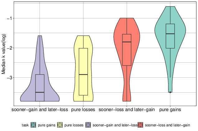
| Figure 1: Violin and box plots of the median k value
(log) for the four discounting tasks, sorted according to the magnitude of
the median k value (log). The crossbar of each box represents the
median; the bottom and top edges of the box represent the first and third
quartiles; the dot represents one data point, which is an extreme outlier.
One data point lies outside the range of this figure in the pure gains
condition. The violin-shaded areas reflect the distribution shape of the
data. |
| Table 3: The effect of possible mechanisms on the discounting rate of four tasks. |
| Tasks: | Pure
gains | Sooner-loss
later-gain | Pure
losses | Sooner-gain
later-loss |
| Present bias | ↑ | - | ↓ | - |
| Status quo effect | - | ↑ | - | ↓ |
| Sequence effect | - | ↓ | - | ↓ |
| Salience account | - | ↓ | - | ↓ |
| Loss aversion | - | ↑ | - | ↓ |
| Debt aversion | - | ↑ | ↓ | ↓ |
As shown in Table 3, we concluded that various effects could contribute to the differences in the discounting rates between the four tasks. The “↑” represents an effect that can help to increase the discount rate in a task, “↓” represents an effect that can help to decrease the discount rate in a task, and “-” represents an effect that does not exist in a task.
Present bias describes a condition in which people are willing to
experience the outcome now rather than in the future regardless of whether
it is positive or negative (Hardisty, Appelt, et al., 2013), which could
help to yield a higher discount rate in the pure gains task and a lower
discount rate in the pure losses task.
The status-quo effect indicates a preference for the current state of
affairs or a tendency to leave a situation unchanged (Lempert & Phelps,
2016; Patty, 2006), which could lead to more rejections in the mixed
tasks, in which participants were asked to keep a status-quo or choose a
prospect. This effect could help to yield the higher discount rate in the
sooner-loss and later-gain task and the lower discount rate in the
sooner-gain and later-loss task.
The sequence effect proposed by Loewenstein and Prelec (1993) posits that
people favor an increasing sequence and disfavor a decreasing sequence. In
our study, the sooner-gain and later-loss task could be identified as a
decreasing sequence, while the sooner-loss and later-gain task may be an
increasing sequence; the sequence effect could help to yield the lower
discount rate of the sooner-gain and later-loss task and the higher
discount rate of the sooner-loss and later-gain task.
The salience account suggests that a discounting rate of intertemporal
sequences is generally (though not always) smaller than that of a
single-dated outcome (Jiang et al., 2014). When choosing between two
single-dated outcomes, people trade off outcomes against delays, and they
may pay equal attention to these two attributes (delay and outcome).
However, when choosing between prospects involving sequences, people may
be more focused on outcomes than on delays because, in sequences, outcomes
are more salient than delays. Thus, choices involving sequences often show
lower discounting rates than choices between single-dated outcomes (Jiang
et al., 2017; Jiang et al., 2016; Jiang et al., 2014; Sun & Jiang, 2015).
In the mixed tasks, prospects can be seen as sequences. Therefore, the
salience account would predict lower discounting rates for the mixed tasks
than for the other two tasks.
Loss aversion refers to the tendency to prefer avoiding losses to acquiring
equivalent gains, which is identified in risky choice rather than
intertemporal choice. Some researchers have borrowed this definition to
construct models of intertemporal choice (Loewenstein & Prelec, 1992;
Scholten & Read, 2010). Loss aversion would predict more rejections in
the mixed tasks, which would help to yield the lower discount rate in the
sooner-gain and later-loss task and the higher discount rate in the
sooner-loss and later-gain task. However, whether loss aversion actually
exists is debatable. Some researchers hold that the current evidence does
not support the view that losses tend to be any more impactful than gains
(Gal & Rucker, 2018).
Debt aversion suggests that people are unwilling to enter into a financial
contract framed or labeled as “debt” (Caetano et al., 2019). This aversion
has been used to explain why people often pay off mortgages and student
loans quicker than they have to (Eckel et al., 2007; Loewenstein & Thaler,
1989). In the mixed and pure losses tasks, the option involves a loss if it
is framed as a debt by participants, which could motivate them to avoid a
loss or pay it off as soon as possible. Therefore, debt aversion could help
to yield the lower discount rates in the pure losses task and sooner-gain
and later-loss task and the higher discount rate in the sooner-loss and
later-gain task.
Ultimately, a discount rate is an end product of mechanisms involving many
psychological factors, which affect the participants involved in different
tasks in various ways. The underlying mechanism of the differences in
discount rates between the four tasks remains an interesting topic for
exploration.
3 Experiment 2: Estimating the
Relations between Discount Rates and Real-world Behaviors and
Consequences
Experiment 1 revealed the differences in discount rates between the four
tasks preliminarily. To make the results more robust, we extended the
sample from students to community individuals in Experiment 2.
Furthermore, we estimated the relations between the four tasks and
real-world behaviors and consequences.
We assumed that any task at least measures some kind of discounting rate.
Thus, we predicted that, for all four tasks, a higher discounting rate was
associated with a lower frequency of floss use, less exercise, larger BMI,
a lack of following a diet, less credit paid in full, a higher frequency of
smoking, a higher frequency of alcohol use, a higher frequency of gambling,
a higher frequency of junk food eating, more time used for entertainment
and social interaction with smartphones, less savings compared to
colleagues, less savings compared to contemporaries, less success compared
to colleagues, and less success compared to contemporaries, largely based
on the literature (Amlung et al., 2017; Chabris et al., 2008; Hardisty,
Thompson, et al., 2013; Mackillop et al., 2011). (See the
supplement for the item wording; the full materials
and data are available at https://osf.io/eq79p/.)
Moreover, we predicted that the discounting rates yielded from the tasks
that represented real-world behaviors and consequences most closely would
be the best predictors of those behaviors and consequences. Specifically,
we predicted that the pure gains task would do better for saving behavior;
the pure losses task would do better for credit paid in full; that
smoking, alcohol use, gambling, junk food eating, and smartphone use for
entertainment would be explained better by the sooner-gain and later-loss
task; and that exercise, floss use, and diet status would be explained
better by the sooner-loss and later-gain task. We made no predictions
about which tasks would be most closely related to BMI and success because
there are too many influencing factors for them.
3.1 Method
Eight hundred and sixty-nine participants were recruited from Sojump
(http://www.sojump.com), a popular online
survey website in China. After completing discounting tasks similar to
those used in Experiment 1, participants were asked to report some of
their personal behaviors and consequences (mostly taken from Chabris et
al. [2008]; listed in Table 5). The order of the two options in the
discounting task items was counterbalanced among participants.
3.2 Results and Discussion
As in Experiment 1, we used an Excel-based program to calculate the
discounting rates. Six participants in the pure gains, 17 participants in
the pure losses, 16 participants in the sooner-loss and later-gain, and 15
participants in the sooner-gain and later-loss conditions who showed an
overall consistency score lower than 75% were excluded. We found no
difference in the exclusion amounts of the four tasks (χ2(3,
N = 869) = 5.9, p = .116). Hence, they were excluded
safely, leaving 815 valid questionnaires4
(316 males, Mage = 30.37, SD = 8.18) for
the final analysis (see Table 4).
| Table 4: Demographic characteristics and k values of the samples. |
| Tasks: | Pure
gains | Pure
losses | Sooner-gain
later-loss | Sooner-loss
later-gain |
| N | 209 | 204 | 197 | 205 |
| Male | 76 (33.4%) | 76 (37.3%) | 81 (41.1%) | 82 (40.0%) |
| Age (SD) | 30.26 (7.80) | 30.59 (8.06) | 30.53 (8.16) | 30.17 (8.68) |
| k value (SD) | 0.0423 (0.0613) | 0.0156 (0.0471) | 0.0129 (0.0492) | 0.0250 (0.0501) |
| Log k value (SD) | −1.84 (0.73) | −2.74 (0.86) | −3.00 (0.83) | −2.21 (0.78) |
3.2.1 Tasks and Discount Rates
The differences in discount rates between the four tasks are consistent
with those in Experiment 1. The four tasks yielded different discount
rates (F (3,811) = 86.88, p < .001,
η2 = 0.243), and post-hoc tests revealed the same order of
discount rates among the four tasks as that found in Experiment 1
(ps < .005).5
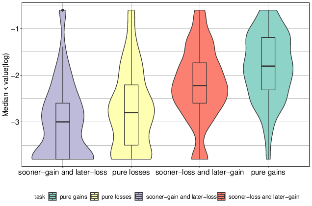
| Figure 2: Violin and box plots of the median k value
(log) for the four discounting tasks, sorted according to the magnitude of
the median k value (log). The crossbar of each box represents the
median; the bottom and top edges of the box represent the first and third
quartiles. One data point lies outside the range of this figure in the
sooner-gain and later-loss condition. The violin-shaded areas reflect the
distribution shape of the data. |
3.2.2 Discount Rates and Real-world Behaviors and Consequences
We reverse-scored several items to make positive values, indicating the
relations in the predictive direction we assumed.6 We ran the liner regressions, and reported the
results in Table 5. The columns show the estimates of the log k
values when the behaviors and consequences are regressed on the demographic
characteristics (i.e., age, age2/100, education, gender
and family income) and the log k value. The complete regression
results are provided at the end of this paper (in the Extended Tables). The
results revealed that the discounting rates from the four tasks cannot
explain the behaviors and consequences except for a few, even some in the
reverse-predictive direction, which remains to be studied. Ultimately, we
found that the evidence supporting a relation between the discount rates of
the four tasks and the different real-world behaviors and consequences was
insufficient.
| Table 5: Regressions estimates of discount rates yielded from four tasks. |
| Tasks: | Pure
gains | Pure
losses | Sooner-gain
later-loss | Sooner-loss
later-gain |
| BMI | 0.15 | 0.07 | -0.14 | -0.01 |
| Exercise§ | 0.06 | -0.07 | -0.06 | -0.31^** |
| Diet status§ | 0.04 | 0.06 | -0.13^** | 0.13^** |
| Floss using§ | -0.10 | 0.15 | -0.27^** | 0.02 |
| Credit paid in full§£ | 0.17 | 0.03 | 0.21^* | -0.22^* |
| Smoking | 0.08 | -0.07 | 0.10 | 0.15 |
| Alcohol using | 0.14 | 0.04 | 0.11 | 0.02 |
| Gambling | 0.07 | -0.09 | 0.30^*** | -0.04 |
| Junk food eating | -0.02 | -0.05 | 0.04 | 0.08 |
| Smartphone using | -0.01 | -0.09 | -0.04 | 0.07 |
| Save / colleague§ | 0.11 | 0.00 | -0.10 | -0.06 |
| Save / contemporary§ | 0.09 | 0.08 | -0.11 | -0.09 |
| Success / colleague§ | 0.05 | 0.01 | -0.08 | -0.17 |
| Success / contemporary§ | 0.16 | 0.01 | -0.10 | -0.10 |
| § These items were reverse-scored so that positive values indicated a
correlation in the predicted direction;£ excluded participants who did
not use any credit tools because we could not arbitrarily classify them as
preferring the present or the future; hence, the samples of the items of
the four tasks are 166, 159, 157, and 163, respectively;
* p < .05; ** p < .01; *** p < .001. |
3.2.3 Pure Gains Task and Real-world Behaviors and Consequences
The evidence from research on the relations between intertemporal choices
of pure gains task in the laboratory and real-world behaviors and
consequences is relatively sufficient; thus, this issue will be discussed
first. In our study, the effects of the discount rate yielded from pure
gains task are statistically insignificant for all behaviors and
consequences. Previous studies based on non-clinical participants have
shown that discount rates are weakly correlated with real-world behaviors
and consequences (Chabris et al., 2008; Daugherty & Brase, 2010;
Sanchez-Roige et al., 2018). For example, Chabris et al. (2008) conducted
three studies to examine the relations between discount rates and
behaviors. Their Study 3, which measured 14 behaviors and consequences in
normal individuals with online questionnaires, is similar to the pure
gains condition in our Experiment 2. The results of their Study 3 showed
that the discounting rate had a positive and significant correlation with BMI and
credit card bill paid in full but a negative and significant relationship with
prescription drug compliance. Our results are not consistent with these.
The main reasons for the difference between the results may be that their
study excluded participants who always chose either the delayed or
immediate rewards and used a larger sample size than that used in our pure
gains condition; moreover, the participants in their study were
incentivized to be incentive compatible. These different measures may have
led to the different results. Although the effects of the discount rates
on all the behaviors and consequences we measured did not reach
statistical significance, most of them were consistent with the expected
directions (only three of the 14 were in the opposite direction).
Therefore, our study is generally consistent with previous studies on the
relations between the discount rate of the pure gains task and real-world
behaviors and consequences.
Some scholars have discussed why the discount rate is weakly related to
real-world behaviors and consequences (Urminsky & Zauberman, 2015). For
example, regarding the complexity of individual behavior, some behaviors,
which are assumed to be intertemporal choices, may not be dominated or
even affected by discount rates. For instance, some people exercise
because the people around them do (like in the herd effect). Once these
social influences exist, people’s decision making does not depend on their
own independent deliberations, and the impact of the discount rate on
real-world outcomes become smaller or even disappears. Furthermore, the
behaviors and consequences considered by researchers to be discount types
are actually not related or are the opposite. For example, some people
always need to balance between working hard for money and exercising, but
it is unreasonable to describe sacrificing exercise in order to work as
short-sighted. After all, making money is also done to obtain a better
life and prepare for the future.
3.2.4 Other Tasks and Real-world Behaviors and Consequences
As Table 5 shows, we found in the pure losses task that the discount rate
could not explain any real-world behavior and consequence, which is
inconsistent with Hardisty, Thompson, et al. (2013). Hardisty, Thompson,
et al. (2013) found that the discount rates yielded from pure losses task
with an alternative titration method could predict some consequential
outcomes (e.g., exercise, credit paid in full). Our results and Hardisty,
Thompson, et al.’s may differ because their study used non-parametric
correlations, while we used regressions and controlled for other
variables; moreover, we used Kirby’s task to yield the discount rate while
they used a self-designed task. For the newly introduced tasks, the
findings are both expected and unexpected. In the sooner-gain and
later-loss task, the discount rate can explain gambling (b =
0.30, p = .001) and credit paid in full (b = 0.21,
p = .024), consistent with our prediction; however, its effects
on diet status (b = −0.13, p = .002) and floss use
(b = −0.27, p = .002) are significant but contrary to
our prediction. In the sooner-loss and later-gain task, the discount rate
can explain diet status (b = 0.13, p = .002), consistent
with our prediction; however, its effects on credit paid in full
(b = −0.22, p = .031) and exercise (b = −0.31,
p = .006) are significant but contrary to our prediction. In
these three tasks, the other relations are not statistically significant,
and a considerable part of the behaviors and consequences (five, nine, and
eight of the 14 outcomes in the pure losses, sooner-gain and later-loss,
and sooner-loss and later-gain tasks) are contrary to our expectations.
It is possible that the discount rate of a pure gains task can
represent a “universal” discount rate, which is related to real behaviors
and consequences, while other tasks cannot. The relations in the two mixed
tasks may be false correlations (false positive errors) caused by multiple
tests. However, other discount tasks may also predict behaviors and
consequences, but our tasks did not include zero or negative discount rate
situations because we used and adjusted Kirby’s discounting task (Kirby et
al., 1999; Kirby, 2009). Previous research has shown that loss outcomes
can yield a negative discount rate (Hardisty, Thompson, et al., 2013). The
results may be different if the tasks can accommodate zero or negative
discount rates.
4 General Discussion
In Experiment 1, we compared mixed gain-loss intertemporal choices with
pure gains or pure losses choices with a college student sample. The
results demonstrated that the discount rate ordering of the four tasks,
from highest to lowest, was pure gains, sooner-loss and later-gain, pure
losses, and sooner-gain and later-loss. In Experiment 2, we repeated the
process for the four tasks with community participants and also measured
their self-reported real-world behaviors and consequences. We found that
the evidence supporting the claim that discount rates from different tasks
are related to different real-world behaviors and consequences was
insufficient.
In both experiments, we used hypothetical tasks rather than real monetary
incentives to yield the discount rates because it is almost impossible for
us to ask participants to pay money in the pure losses and mixed tasks.
Fortunately, previous studies have shown that there are no differences
between real and hypothetical intertemporal outcomes at the behavioral
level (Johnson & Bickel, 2002; Madden et al., 2003) or neural level
(Bickel et al., 2007).
We have confidence in our finding that different tasks yield different
discount rates. The results of this study further the research on
gain-loss asymmetry. However, more research is needed to explore the
relations between the discount rates of different tasks and real-world
behaviors and consequences.
References
Amlung, M., Vedelago, L., Acker, J., Balodis, I., & MacKillop, J. (2017).
Steep delay discounting and addictive behavior: A meta-analysis of
continuous associations. Addiction, 112(1), 51–62.
Bickel, W. K., Miller, M. L., Yi, R., Kowal, B. P., Lindquist, D. M., &
Pitcock, J. A. (2007). Behavioral and neuroeconomics of drug addiction:
competing neural systems and temporal discounting processes. Drug
and Alcohol Dependence, 90 (Suppl 1), S85.
Caetano, G., Palacios, M., & Patrinos, H. A. (2019). Measuring aversion to
debt: An experiment among student loan candidates. Journal of
Family and Economic Issues, 40(1), 117–131.
Chabris, C. F., Laibson, D., Morris, C. L., Schuldt, J. P., & Taubinsky,
D. (2008). Individual laboratory-measured discount rates predict field
behavior. Journal of Risk and Uncertainty, 37(2-3), 237–269.
Cohen, J., Ericson, K. M., Laibson, D., & White, J. M. (2020). Measuring
time preferences. Journal of Economic Literature, 58(2), 299–347.
Daugherty, J. R., & Brase, G. L. (2010). Taking time to be healthy:
Predicting health behaviors with delay discounting and time perspective.
Personality and Individual Differences, 48(2), 202–207.
Eckel, C. C., Johnson, C., Montmarquette, C., & Rojas, C. (2007). Debt
aversion and the demand for loans for postsecondary education.
Public Finance Review, 35(2), 233–262.
Estle, S. J., Green, L., & Myerson, J. (2019). When immediate losses are
followed by delayed gains: Additive hyperboloid discounting models.
Psychonomic Bulletin & Review, 26(4), 1418–1425.
Franco-Watkins, A. M., Mattson, R. E., & Jackson, M. D. (2016). Now or
later? Attentional processing and intertemporal choice. Journal of
Behavioral Decision Making, 29(2-3), 206–217.
Freeman, D., Manzini, P., Mariotti, M., & Mittone, L. (2016). Procedures
for eliciting time preferences. Journal of Economic Behavior &
Organization, 126, 235–242.
Frederick, S., Loewenstein, G., & O’donoghue, T. (2002).
Time discounting and time preference: A critical review. Journal
of Economic Literature, 40(2), 351–401.
Gal, D., & Rucker, D. D. (2018). The loss of loss aversion: Will it loom
larger than its gain?. Journal of Consumer Psychology, 28(3),
497–516.
Hardisty, D. J., Appelt, K. C., & Weber, E. U. (2013). Good or bad, we
want it now: Fixed-cost present bias for gains and losses explains
magnitude asymmetries in intertemporal choice. Journal of
Behavioral Decision Making, 26(4), 348–361.
Hardisty, D. J., Thompson, K. F., Krantz, D. H., & Weber, E. U. (2013).
How to measure time preferences: An experimental comparison of three
methods. Judgment and Decision Making, 8(3), 236–249.
Irvine, M. A., Yulia, W., Sorcha, B., Harrison, N. A., Bullmore, E. T., &
Valerie, V., et al. (2013). Impaired decisional impulsivity in
pathological videogamers. PLoS ONE, 8(10), e75914.
Jiang, C. M., Hu, F. P., & Zhu, L. F. (2014). Introducing upfront losses
as well as gains decreases impatience in intertemporal choices with
rewards. Judgment and Decision Making, 9(4), 297–302.
Jiang, C.-M., Sun, H.-M., Zhu, L.-F., Zhao, L., Liu, H.-Z., & Sun, H.-Y.
(2017). Better is worse, worse is better: Reexamination of violations of
dominance in intertemporal choice. Judgment and Decision Making,
12(3), 253–259.
Jiang, C. M., Sun, H. Y., Zheng, S. H., Wang, L. J., & Qin, Y. (2016).
Introducing upfront money can decrease discounting in intertemporal
choices with losses. Frontiers in Psychology, 7, 1256.
Johnson, M. W., & Bickel, W. K. (2002). Within-subject comparison of real
and hypothetical money rewards in delay discounting. Journal of
the Experimental Analysis of Behavior, 77(2), 129–146.
Kaplan, B. A., Amlung, M., Reed, D. D., Jarmolowicz, D. P., McKerchar, T.
L., & Lemley, S. M. (2016). Automating scoring of delay discounting for
the 21- and 27-item monetary choice questionnaires. The Behavior
Analyst / MABA, 39(2), 1–12.
Kirby, K. N. (2009). One-year temporal stability of delay-discount rates.
Psychonomic Bulletin & Review, 16(3), 457–462.
Kirby, K. N., Petry, N. M., & Bickel, W. K. (1999). Heroin addicts have
higher discount rates for delayed rewards than non-drug-using
controls. Journal of Experimental Psychology: General, 128(1), 78–87.
Lempert, K. M., & Phelps, E. A. (2016). The malleability of intertemporal
choice. Trends in Cognitive Sciences, 20(1), 64–74.
Loewenstein, G., & Prelec, D. (1992). Anomalies in Intertemporal Choice:
Evidence and an Interpretation. The Quarterly Journal of
Economics, 107(2), 573–597.
Loewenstein, G., & Prelec, D. (1993). Preferences for sequences of
outcomes. Psychological Review, 100(1), 91–108.
Loewenstein, G., & Thaler, R. H. (1989). Anomalies: intertemporal choice.
Journal of Economic Perspectives, 3(4), 181–193.
MacKillop, J., Amlung, M. T., Few, L. R., Ray, L. A., Sweet, L. H., &
Munafò, M. R. (2011). Delayed reward discounting and addictive behavior: a
meta-analysis. Psychopharmacology, 216(3), 305–321.
Madden, G. J., Begotka, A. M., Raiff, B. R., & Kastern, L. L. (2003).
Delay discounting of real and hypothetical rewards. Experimental
and Clinical Psychopharmacology, 11(2), 139–145.
Mazur, J. E. (1987). An adjusting procedure for studying delayed
reinforcement. In M. L. Commons, J. E. Mazur, J. A. Nevin, & H. Rachlin
(Eds.), Quantitative analyses of behavior: Vol. 5. The effect of
delay and of intervening events on reinforcement value (pp. 55-73).
Hillsdale, NJ: Erlbaum.
Myerson, J., Green, L., & Warusawitharana, M. (2001). Area under the curve
as a measure of discounting. Journal of The Experimental Analysis
of Behavior, 76(2), 235–243.
Mole, T. B., Irvine, M. A., Worbe, Y., Collins, P., Mitchell, S. P., &
Bolton, S., et al. (2015). Impulsivity in disorders of food and drug
misuse. Psychological Medicine, 45(04), 771–782.
Ostaszewski, P. (2007). Temporal discounting in “gain
now-lose later” and “lose now-gain
later” conditions. Psychological Reports,100(2),
653–660.
Patty, J. W. (2006). Loss aversion, presidential responsibility, and
midterm congressional elections. Electoral Studies, 25(2),
227–247.
Read, D., & Roelofsma, P. (2003). Subadditive versus hyperbolic
discounting: A comparison of choice and matching. Organizational
Behavior & Human Decision Processes, 91, 140–153.
Reynolds, B., & Fields, S. (2012). Delay discounting by adolescents
experimenting with cigarette smoking. Addiction, 107(2), 417–424.
Sanchez-Roige, S., Fontanillas, P., Elson, S. L., Pandit, A., Schmidt, E.
M., Foerster, J. R., ... & MacKillop, J. (2018). Genome-wide association
study of delay discounting in 23,217 adult research participants of
European ancestry. Nature Neuroscience, 21(1), 16–18.
Scholten, M., & Read, D. (2010). The psychology of intertemporal
tradeoffs. Psychological Review, 117(3), 925–944.
Sun, H. Y., & Jiang, C. M. (2015). Introducing money at any time can
reduce discounting in intertemporal choices with rewards: an extension of
the upfront money effect. Judgment and Decision Making, 10(6),
564–570.
Thaler, R. (1981). Some empirical evidence on dynamic inconsistency.
Economics Letters, 8(3), 201–207.
Urminsky, O., & Zauberman, G. (2015). The psychology of intertemporal
preferences. In Keren G., & Wu G. (Eds.), The Wiley-Blackwell
handbook of judgment and decision making (pp. 141–181). Chichester, UK:
John Wiley & Sons.
Appendix
Extended Table 1. Real-world behaviors and consequences regression in pure
gains task (s.e. in parentheses).
| Predictor | BMI | Exercise§ | Diet§ | Floss§ | Credit§£ | Smoke | Alcohol | Gamble | Junk food | Phone | Save.1§ | Save.2§ | Suc.1§ | Suc.2§ |
| Log k | 0.15 (0.08) | 0.06 (0.09) | 0.04 (0.05) | −0.10 (0.09) | 0.08 (0.07) | 0.17 (0.11) | 0.14 (0.09) | 0.07 (0.10) | −0.02 (0.10) | −0.01 (0.09) | 0.11 (0.10) | 0.09 (0.09) | 0.05 (0.09) | 0.16 (0.09) |
| Age | 0.91** (0.34) | −0.49 (0.40) | −0.18 (0.20) | −0.80* (0.41) | −0.64* (0.31) | 0.81 (0.63) | 0.49 (0.38) | 0.56 (0.41) | −0.76 (0.43) | −1.14** (0.39) | −0.43 (0.42) | −0.06 (0.40) | 0.43 (0.39) | 0.32 (0.39) |
| Age2/100 | −0.69* (0.35) | 0.56 (0.41) | 0.18 (0.20) | 0.82* (0.42) | 0.87** (0.32) | −0.96 (0.68) | −0.31 (0.39) | −0.56 (0.43) | 0.65 (0.44) | 0.92* (0.40) | 0.57 (0.43) | 0.08 (0.41) | −0.51 (0.40) | −0.41 (0.40) |
| Education | −0.03 (0.06) | 0.01 (0.08) | 0.00 (0.04) | 0.01 (0.08) | −0.02 (0.06) | −0.15 (0.09) | 0.02 (0.07) | −0.08 (0.08) | 0.08 (0.08) | 0.07 (0.07) | −0.05 (0.08) | −0.16* (0.08) | −0.28*** (0.07) | −0.25** (0.07) |
| Gender(male) | 0.65*** (0.12) | −0.25 (0.14) | −0.06 (0.07) | 0.04
(0.15) | 0.44*** (0.11) | −0.18 (0.17) | 0.59*** (0.14) | 0.30* (0.15) | −0.26 (0.16) | −0.08 (0.14) | −0.10 (0.15) | 0.01 (0.14) | 0.08 (0.14) | 0.02 (0.14) |
| Family income | −0.11 (0.06) | −0.14 (0.07) | −0.06 (0.04) | −0.20** (0.07) | 0.10 (0.06) | −0.02 (0.09) | 0.09 (0.07) | −0.01 (0.07) | 0.17* (0.08) | 0.03 (0.07) | −0.19* (0.08) | −0.24** (0.07) | −0.36*** (0.07) | −0.40*** (0.07) |
| Observations | 209 | 209 | 209 | 209 | 166 | 209 | 209 | 209 | 209 | 209 | 209 | 209 | 209 | 209 |
| R2 | 0.243 | 0.050 | 0.034 | 0.070 | 0.056 | 0.202 | 0.170 | 0.032 | 0.062 | 0.096 | 0.070 | 0.093 | 0.201 | 0.222 |
Extended Table 2. Real-world behaviors and consequences regression in pure
losses task (s.e. in parentheses).
| Predictor | BMI | Exercise§ | Diet§ | Floss§ | Credit§£ | Smoke | Alcohol | Gamble | Junk food | Phone | Save.1§ | Save.2§ | Suc.1§ | Suc.2§ |
| Log k | 0.07 (0.07) | −0.07 (0.07) | 0.06 (0.04) | 0.15 (0.08) | 0.03 (0.11) | −0.07 (0.08) | 0.04 (0.08) | −0.09 (0.09) | −0.05
(0.08) | −0.09 (0.09) | 0.00 (0.08) | 0.08 (0.08) | 0.01 (0.08) | 0.01 (0.08) |
| Age | −0.08 (0.30) | −0.16 (0.30) | −0.22 (0.18) | −0.04 (0.36) | 0.94 (0.72) | 0.17 (0.35) | 0.38 (0.38) | 0.51 (0.40) | −0.84* (0.34) | −0.74 (0.40) | −0.14 (0.35) | −0.11 (0.37) | 0.16 (0.37) | 0.51 (0.35) |
| Age2/100 | 0.27 (0.29) | 0.11 (0.30) | 0.18 (0.18) | −0.09 (0.35) | −1.08 (0.74) | −0.09 (0.34) | −0.32 (0.37) | −0.48 (0.39) | 0.56 (0.33) | 0.63 (0.39) | 0.11 (0.35) | 0.15
(0.36) | −0.24 (0.36) | −0.51 (0.34) |
| Education | 0.02 (0.06) | 0.00 (0.06) | 0.03 (0.03) | −0.13 (0.07) | −0.07 (0.11) | −0.05 (0.07) | −0.02 (0.07) | −0.08 (0.08) | −0.01 (0.07) | −0.05 (0.08) | 0.11 (0.07) | 0.09 (0.07) | 0.01
(0.07) | −0.04 (0.07) |
| Gender(male) | 0.46*** (0.12) | −0.22 (0.12) | −0.12 (0.07) | −0.03 (0.14) | 0.25 (0.17) | 0.83*** (0.14) | 0.55*** (0.15) | 0.48** (0.15) | −0.08 (0.13) | −0.16 (0.15) | −0.16 (0.14) | −0.33* (0.14) | −0.28 (0.14) | −0.26 (0.13) |
| Family income | −0.08 (0.06) | −0.15* (0.06) | −0.09* (0.04) | −0.21** (0.07) | −0.08 (0.11) | −0.04 (0.07) | 0.13 (0.08) | 0.02 (0.08) | 0.05 (0.07) | 0.02 (0.08) | −0.41*** (0.07) | −0.36*** (0.08) | −0.29*** (0.07) | −0.37*** (0.07) |
| Observations | 204 | 204 | 204 | 204 | 159 | 204 | 204 | 204 | 204 | 204 | 204 | 204 | 204 | 204 |
| R2 | 0.154 | 0.082 | 0.082 | 0.115 | 0.036 | 0.176 | 0.111 | 0.062 | 0.116 | 0.050 | 0.170 | 0.134 | 0.110 | 0.163 |
Extended Table 3. Real-world behaviors and consequences regression in
sooner-gain and later-loss task (s.e. in parentheses).
| Predictor | BMI | Exercise§ | Diet§ | Floss§ | Credit§£ | Smoke | Alcohol | Gamble | Junk food | Phone | Save.1§ | Save.2§ | Suc.1§ | Suc.2§ |
| Log k | −0.14 (0.10) | −0.06 (0.08) | −0.13** (0.04) | −0.27** (0.09) | 0.21* (0.09) | 0.10 (0.08) | 0.11 (0.08) | 0.30*** (0.09) | 0.04 (0.09) | −0.04 (0.09) | −0.10 (0.08) | −0.11 (0.08) | −0.08 (0.08) | −0.10 (0.08) |
| Age | 0.76 (0.45) | −0.19 (0.38) | −0.08 (0.19) | −0.77 (0.40) | 0.01 (0.50) | 1.00* (0.39) | 0.61 (0.37) | 1.14** (0.42) | −0.42 (0.42) | 0.57 (0.42) | 0.18 (0.37) | 0.57 (0.37) | 0.61 (0.39) | 0.56 (0.38) |
| Age2/100 | −0.53 (0.45) | 0.13 (0.39) | 0.13 (0.19) | 0.80* (0.40) | −0.21 (0.50) | −0.92* (0.39) | −0.57 (0.37) | −1.13** (0.42) | 0.25 (0.43) | −0.64 (0.42) | −0.09 (0.37) | −0.47 (0.37) | −0.56 (0.39) | −0.52 (0.38) |
| Education | −0.08 (0.08) | 0.03 (0.07) | −0.04 (0.03) | −0.07 (0.07) | −0.17 (0.09) | −0.14* (0.07) | 0.12 (0.06) | −0.04 (0.07) | −0.02 (0.07) | 0.10 (0.07) | −0.05 (0.06) | −0.10 (0.06) | −0.11 (0.07) | 0.01 (0.07) |
| Gender(male) | 0.52** (0.17) | −0.05 (0.14) | 0.05 (0.07) | 0.20 (0.15) | −0.11 (0.16) | 1.18*** (0.14) | 0.59*** (0.14) | 0.22 (0.15) | −0.31 (0.16) | −0.06 (0.16) | −0.06 (0.14) | −0.22 (0.14) | −0.15 (0.14) | −0.06 (0.14) |
| Family income | −0.15 (0.08) | −0.12 (0.07) | −0.02 (0.03) | −0.06 (0.07) | −0.01 (0.08) | 0.02 (0.07) | 0.15* (0.07) | 0.00 (0.08) | −0.01 (0.08) | −0.10 (0.08) | −0.15* (0.07) | −0.22** (0.07) | −0.26*** (0.07) | −0.27*** (0.07) |
| Observations | 197 | 197 | 197 | 197 | 157 | 197 | 197 | 197 | 197 | 197 | 197 | 197 | 197 | 197 |
| R2 | 0.134 | 0.031 | 0.083 | 0.097 | 0.096 | 0.337 | 0.186 | 0.118 | 0.060 | 0.037 | 0.046 | 0.098 | 0.099 | 0.085 |
Extended Table 4. Real-world behaviors and consequences regression in
sooner-loss and later-gain task (s.e. in parentheses).
| Predictor | BMI | Exercise§ | Diet§ | Floss§ | Credit§£ | Smoke | Alcohol | Gamble | Junk food | Phone | Save.1§ | Save.2§ | Suc.1§ | Suc.2§ |
| Log k | −0.01 (0.09) | −0.31** (0.11) | 0.13** (0.04) | 0.02 (0.09) | −0.22* (0.10) | 0.15 (0.08) | 0.02 (0.08) | −0.04 (0.08) | 0.08 (0.08) | 0.07 (0.08) | −0.06 (0.09) | −0.09 (0.09) | −0.17 (0.09) | −0.10 (0.09) |
| Age | 0.22 (0.36) | −0.51 (0.43) | 0.05 (0.16) | −0.67 (0.36) | −0.69 (0.57) | 0.38 (0.31) | 0.98** (0.33) | 0.27 (0.31) | −0.54 (0.33) | −0.39 (0.33) | −0.31 (0.35) | −0.18 (0.37) | −0.21 (0.34) | 0.51 (0.35) |
| Age2/100 | −0.13 (0.35) | 0.33 (0.42) | −0.07 (0.16) | 0.63 (0.35) | 0.72 (0.60) | −0.31 (0.30) | −0.86** (0.32) | −0.25 (0.30) | 0.28 (0.32) | 0.18 (0.32) | 0.10 (0.35) | 0.07 (0.36) | 0.17 (0.33) | −0.57 (0.34) |
| Education | −0.01 (0.08) | −0.09 (0.10) | 0.01 (0.04) | −0.08 (0.08) | −0.20 (0.10) | 0.04 (0.07) | 0.09 (0.07) | 0.00 (0.07) | 0.05 (0.07) | 0.14 (0.07) | −0.18* (0.08) | −0.10 (0.08) | −0.12 (0.08) | −0.11 (0.08) |
| Gender(male) | 0.73*** (0.15) | 0.22 (0.18) | 0.03 (0.07) | 0.03 (0.15) | −0.15 (0.16) | 0.95*** (0.13) | 0.63*** (0.14) | 0.37** (0.13) | −0.04 (0.14) | 0.08 (0.14) | 0.14 (0.15) | 0.06 (0.15) | 0.15 (0.14) | 0.07 (0.14) |
| Family income | 0.04 (0.08) | 0.07 (0.10) | −0.05 (0.04) | −0.06 (0.08) | −0.05 (0.09) | 0.13 (0.07) | 0.05 (0.07) | 0.11 (0.07) | 0.04 (0.07) | −0.15* (0.07) | −0.22** (0.08) | −0.21** (0.08) | −0.20** (0.08) | −0.26** (0.08) |
| Observations | 205 | 205 | 205 | 205 | 163 | 205 | 205 | 205 | 205 | 205 | 205 | 205 | 205 | 205 |
| R2 | 0.147 | 0.057 | 0.078 | 0.047 | 0.076 | 0.282 | 0.187 | 0.074 | 0.104 | 0.119 | 0.143 | 0.081 | 0.101 | 0.085 |
Notes for Extended Table 1-4: § and £ have the same meanings as those
given in Table 5 in the paper; * p < .05; ** p
< .01; *** p < .001
This document was translated from LATEX by
HEVEA.