Judgment and Decision Making, Vol. 16, No. 3, May 2021, pp. 687-708
Misjudgment of interrupted time-series graphs due to serial dependence: Replication of Matyas and Greenwood (1990)
Anthony J. Bishara*
Jacob Peller#
Chad M. Galuska$
|
Abstract:
Interrupted time-series graphs are often judged by eye. Such a graph might show,
for example,
patient symptom severity (y) on each of several
days (x) before and after a treatment was implemented
(interruption). Such graphs might be prone to systematic misjudgment
because of serial dependence, where random error at each timepoint persists
into later timepoints. An earlier study (Matyas & Greenwood, 1990) showed
evidence of systematic misjudgment, but that study has often been
discounted due to methodological concerns. We address these concerns and
others in two experiments. In both experiments, serial dependence increased
mistaken judgments that the interrupting event led to a change in the
outcome, though the pattern of results was less extreme than in previous
work. Receiver operating characteristics suggested that serial dependence
both decreased discriminability and increased the bias to decide that the
interrupting event led to a change. This serial dependence effect appeared
despite financial incentives for accuracy, despite feedback training, and
even in participants who had graduate training relevant to the task.
Serial dependence could cause random error to be misattributed to real
change, thereby leading to judgments that interventions are effective even
when they are not.
Keywords: serial dependence, time series, graphs, discontinuity
1 Introduction
The science of human judgment provides numerous examples of people
“discovering” patterns where none exist (Baron, 2008; Gilovich, 1991;
Vyse, 2013). Famous examples include illusory associations in judgments
about people (Chapman & Chapman, 1969; Hamilton & Rose, 1980), locations
(Clarke, 1946), or other stimuli (Chapman, 1967). Here, we consider the
potential for illusory correlation in judgment of a common type of graph —
an interrupted time-series graph — where viewers judge whether an
interrupting event is associated with a change in the
subsequent height of the data points. Such graphs are common in many
parts of life, for example, in news articles claiming that a stock market
“tumbles on” some major incident or prominent figure’s comments.
Relatedly, at the time of this writing, these graphs are being judged to
infer whether health policy implementation was followed by a change in
disease infection rate. These graphs are also common in single-subject
(n=1) A-B designs, where the comparison is between data points
before versus after some intervention on a single participant. In addition
to being common, these graphs can be useful in the study of covariation
detection because they are relatively simple. Unlike stimuli that are
slowly revealed over the course of an experiment (e.g., Chapman &
Chapman, 1969), graphs provide a static display of all relevant
information at once, avoiding complications of forgetting and memory
biases. Another simplification is that only one of the relevant variables
is continuous (data height); the other is binary (before-versus-after the
interruption). Hence, judgment of these graphs can be viewed as
point-biserial correlation detection. Despite the simplicity of these
graphs, we worry that they are especially prone to misjudgment because of
a common attribute of time-series data: serial dependence.
One example of serial dependence is that warm days tend to be followed by
warm days, and cold by cold. This pattern can be seen, for instance, when
examining daily high temperatures of New York City’s Central Park for each
day in January 2020 (National Centers for Environmental Information,
2020). Perhaps the simplest measure of serial dependence is the lag-1
autocorrelation, and those temperatures show an autocorrelation of
r = .54. This autocorrelation is just the correlation between
the temperature on each day and the day that follows it (Jan. 1 paired
with 2, 2 with 3, and so on). Non-zero autocorrelation is also common in
time-series of behavior. An analysis of psychology and education journals
from 2008 found that single case design datasets had a mean
autocorrelation of +.20 (bias corrected; Shadish & Sullivan, 2011).
Serial dependence also varied across studies and types of designs. For
example, the simplest designs (e.g., 10 trials of condition A followed by
10 trials of condition B) had relatively high serial dependence with a
mean autocorrelation of .75, whereas alternating treatment designs — in
which the condition can change on every trial (e.g., ABABBA) — had a mean
autocorrelation of -.01 on average.
To visualize serial dependence, consider a simplified scenario where some
outcome is measured over 6 days, with an intervention occurring
between the 3rd and 4th days. Even if the intervention has no effect, one
could expect some fluctuation in the outcome due to random error. The top
panel of Figure 1 illustrates a situation where random error is independent
across days. The gray dashed horizontal line at a height of 10 indicates
the baseline (error-free) outcome. Relative to this baseline, error may
increase or decrease the outcome measure, as indicated by arrows and
the e corresponding to each day. Without serial dependence, error on one
day affects the outcome only on that day. In other words, error on each day
is independent of error on other days. A large random error immediately
after the intervention (4) will alter the outcome, but just for a single
measurement. So, without serial dependence, it is apparent that the
intervention is not associated with any meaningful change. The temporary
increase in the outcome on day 4 would likely be judged correctly as random
noise rather than systematic change produced by the intervention.
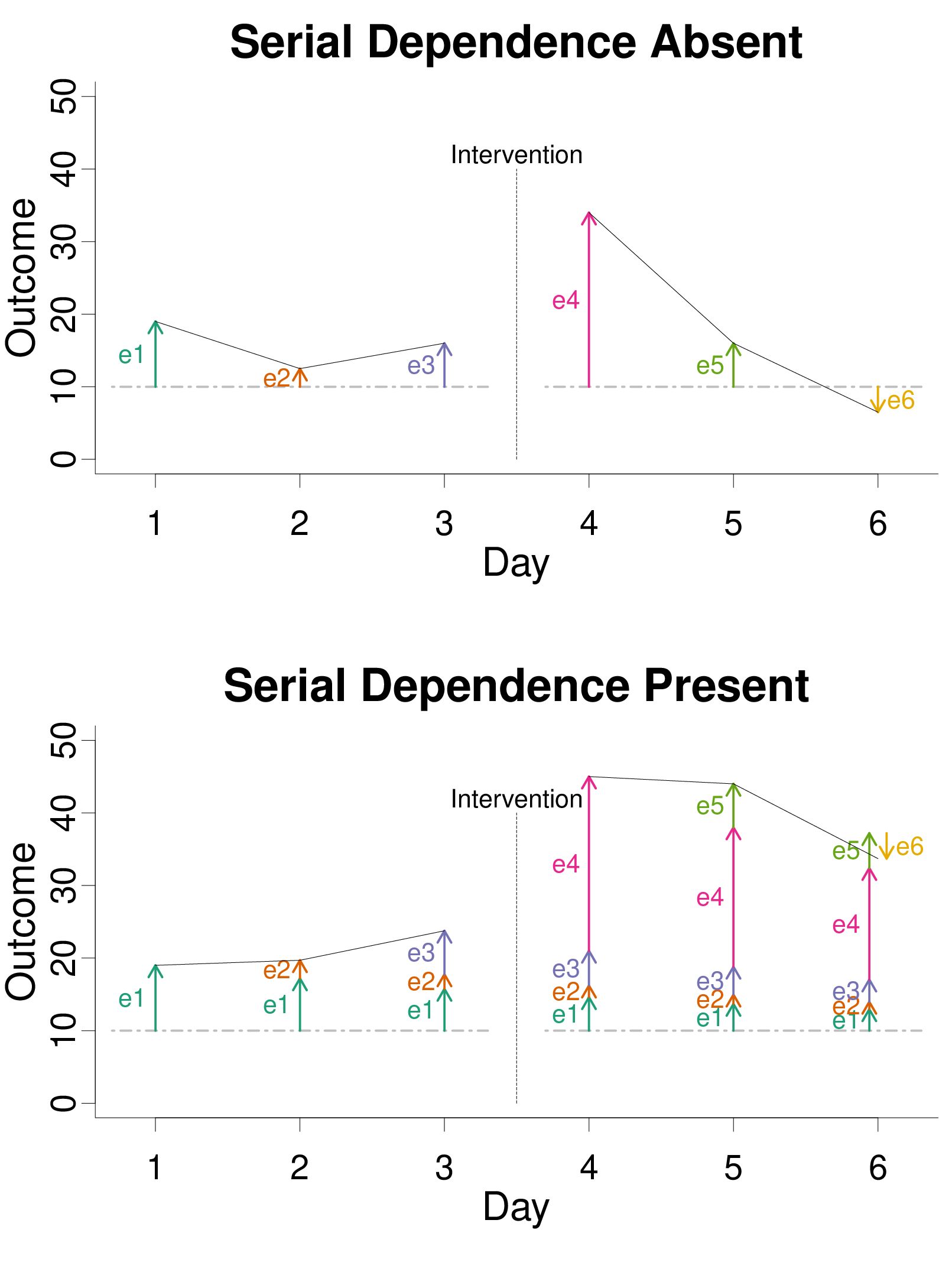
| Figure 1: Illustration of the impact of random error and serial dependence
in a situation where the intervention has no effect (i.e., the Null
Hypothesis is true). When serial dependence is absent, error (colored
arrows labelled with e) at each time point has no effect on other time
points. In contrast, when serial dependence is present, error on each day
persists with diminishing effect on the days that follow. The horizontal
dashed line indicates an error-free baseline. |
As illustrated in the bottom panel of Figure 1, serial dependence can cause
error on one day to persist for the following days, decreasing in its
influence over time. One can see, for example, that the large error on day
4 (e4) impacts the outcomes in the days that follow it. For illustration
purposes, Figure 1 was generated with an extreme serial dependence, with a
1-lag autoregression parameter set to .8. With this setting, error on day 4
is still 80% (i.e., .81) as impactful one day later, 64% (.82) as
impactful two days later, and so on. There are a wide variety of time
series models, but in the simple one considered here, autoregression
parameters typically range from −1 to +1, with values closer to 0
indicating less serial dependence, and a value of exactly 0 indicating its
absence. The lag-1 autocorrelation will be identical to the lag-1
autoregression parameter, at least in the long-run.
In the example at the bottom of Figure 1, serial dependence could create
the illusion of a durable change in the outcome. That is, because the
effect of error persists over time, error could be misattributed to an
effect of the interrupting event, even when the Null hypothesis (no effect)
is true. In other words, a non-zero autocorrelation could create the
illusion of a nonzero-correlation between data height and phase
(before-versus-after the intervention). Incorrectly judging the data
height as being associated with the intervention could be described as a
Type-I error. The phrase “Type I error” often refers to false positives
from mechanical decision rules, most commonly formal statistical hypothesis
tests. Here, we use the phrase more broadly to include false positives in
informal intuitive judgment (e.g., Bishara et al., 2021). The informal
judgment of interest here involves visually inspecting a graph to judge the
association between the intervention and data point height.
Type I errors in informal judgment could plausibly result from serial
dependence. Serial dependence allows random error to temporarily steer
measurements upward or downward, giving the appearance of a stable change
in the height of data points. This effect could increase the chances of
large absolute differences between phases of an intervention. If viewers
relied on a simple heuristic, comparing the average before versus after,
they would be more likely to make Type-I errors. Such a heuristic has been
found in related judgments where people compare two sets of numbers (e.g.,
ratings of two products). For such judgments, people tend to weigh the mean
difference much more than they weigh other relevant cues, such as sample
size or standard deviation (Obrecht et al., 2007).
Even if people were aware that serial dependence could
influence their judgments, it is not clear how they would informally
estimate serial dependence and adjust for it when visually inspecting
graphical displays of data. For example, positive autocorrelation often
leads to visually smoother times-series plots, but so does low noise
(i.e., small residuals), and so it is not clear how serial dependence and
noise would be distinguished. Furthermore, even if people were able to
somehow estimate serial dependence by visually inspecting a graph, they
would still have to adjust their judgments properly. Unfortunately, people
can have inaccurate lay intuitions about serial dependence and evidentiary
value. For example, people sometimes believe that dependent information
provides stronger evidence than independent information even when the
reverse is true (Xie & Hayes, 2020). This belief would lead to
adjustments in the wrong direction.
Some work has already hinted that serial dependence increases Type-I errors
in interrupted time-series graph judgments. Harrington and Velicer (2015)
compared expert graph judgment to statistical analysis of actual data
published in the Journal of Applied Behavior Analysis. This
journal was of particular interest because some applied behavior analysts
prefer informal judgments of graphs in place of formal statistical tests
(also see Smith, 2012), perhaps due to B. F. Skinner’s (1956) skepticism
of the latter. When informal judgments of the articles’ authors clashed
with statistical test results, serial dependence was usually present (also
see Jones et al., 1978). Furthermore, in these clashing cases, graph
judgment often resulted in a determination of significant treatment
effects even when statistical analysis did not. Such results could
suggest that graph judgment amidst serial dependence leads to Type I
errors, but only if one assumes that the statistical analysis was accurate
and graph judgment was not. Unfortunately, with real samples of data, one
does not know whether the treatment effect exists in the population or
not. So, these inconsistencies could indicate Type I errors via graph
judgment, but they could also indicate Type II errors (missing a true
effect) via statistical analysis.
To objectively identify errors, it is necessary to know the population from
which the graph data were generated. If, in the population, there is no
difference before versus after the intervention, then deciding that there
is a treatment effect is truly a Type I error. Matyas and Greenwood
(1990) took this approach, using populations with and without treatment
effects to generate line graphs of A-B designs. When participants judged
these graphs, they frequently made Type I errors, and especially so amidst
serial dependence. When the serial dependence was created with an
autoregressive coefficient of just .3, the Type I error rate was as high
as 84%. To put this number in context, it is useful to compare it to
another practice known to inflate Type I errors: p-hacking.
P-hacking refers to a variety of questionable statistical practices, for
example, repeatedly analyzing data and adding participants until a
p-value happens to stray below .05, at which point the
experiment is stopped (John et al., 2012; Simmons et al., 2011). One
classic simulation study showed that a simultaneous combination of four
different p-hacking techniques inflated Type I error rates from the
intended 5% up to 61% (Simmons et al., 2011), a dangerously high number,
though still not as high as the number in Matyas and Greenwood.
Even setting aside the unusually high Type I error rate, the Matyas and
Greenwood (1990) experiment attracted skepticism for several
methodological reasons. First, in that experiment, the response options
did not allow for different degrees of certainty that a treatment effect
had occurred (Brossart et al., 2006; Parsonson & Baer, 1992). Instead,
participants had five response options: A. no intervention effect, B. a
level change, C. a trend change, D. combined level and trend change, and
E. other type of systematic change during intervention. Thus,
participants had to choose between no-change (A), and change (B-E), but
could not express varying degrees of certainty about whether change
happened. So, it is unclear whether the Type I errors occurred with high
confidence, or merely when participants were guessing.
Second, each condition was represented by just one graph, so if that one
graph happened to have sampling error in the shape of an intervention
effect, then the Type I error rate would be artificially inflated for that
condition (Fisher et al., 2003). In fact, the one graph that produced the
most extreme Type I error rate (84%) by informal judgments also produces
a Type I error when analyzed by a common statistical model (Fisher et al.,
2003). So, that extreme Type I error rate could simply be an artifact of
sampling error in graph generation.
Third, when examining the equation used to generate the graphs (Matyas &
Greenwood, 1990, p. 343), we noticed that there is an alternative
explanation of the increased Type I errors amidst serial dependence. Even
when there is no treatment effect in that equation, it creates on-average
differences between baseline and intervention periods. Those differences
could cause participants to choose something other than “no
intervention effect,” thereby inflating the Type I error
rate. Importantly, this problem arises only when there is serial
dependence, and so this problem could account for the elevated Type I
error rates in that condition (see Appendix for a proof that the expected
difference was non-zero even under the Null Hypothesis).
Fourth, in the Matyas and Greenwood experiment, 50% of graphs had no
effect in them, but only 20% of options (option A) indicated no effect.
If participants inferred that they should spread their responses equally
among options A through E, that incorrect inference could have inflated
Type I errors generally, for all conditions. Although this concern cannot
account for the relatively high Type I errors amidst serial dependence, at
first glance, it could account for the high absolute error rate.
There have been no published attempts to address reasons for skepticism of
Matyas and Greenwood (1990), despite the surprisingly high Type I error
rate observed in that study. We conducted two experiments to do so, one
with a general adult sample, and one with a sample of graduate students
who already had training relevant to the task. Because results were nearly
identical across experiments, findings are presented in a single Results
section.
The primary question of interest was whether Type I errors were more common
when serial dependence was present in the graphs than when it was absent,
and if so, would this pattern merely reflect guesses, or also more
confident responses. Several secondary questions were also considered.
If serial dependence increases Type I errors, could this be due to a
heuristic where people compare the average before versus after the
intervention? Does serial dependence create a bias to decide “treatment”,
or decrease people’s ability to distinguish between treatments and
non-treatments, or both? Additionally, do the absolute rates of Type I
errors reach the extremes indicated by Matyas and Greenwood (84%); are
they elevated even relative to the customary statistical standard (5%)?
Finally, how well do people’s predictions about their performance align
with reality?
2 Experiment 1 Method
2.1 Participants
Initially, 54 adult participants were recruited through Amazon Mechanical
Turk, with the restrictions that they were in the United States and had a
worker rating above 90%. Prior to unblinding to condition, we decided to
exclude any participants performing below chance (.50 correct) overall,
having a median response time under 1 second, or an experiment completion
time of over two hours, as these could demonstrate a lack of attention to
the task. These rules resulted in the exclusion of 4 participants for a
final sample size of n=50 (32 male). Age ranged from 21 to 56
(M = 34.0, SD = 7.37). Participants were paid $5 plus
a bonus that ranged between $0 and $7.20 depending on performance.
2.2 Design and Materials
A 2 (Serial Dependence Absent vs. Present) x 2 (Treatment Effect vs. No
Treatment Effect) repeated-measures factorial design was used. Both
factors were manipulated through the graph generating equations.
Specifically, graphs were generated using a 1-lag autoregressive
interrupted time series model:
where yt was the observed score at time t (see Figure 1). Each graph
had 20 data points (t ranged from 1 to 20). Reviews of actual
single-case designs have found a similar number of datapoints, with medians
of 19 to 20 data points (Harrington & Velicer, 2015; Shadish & Sullivan,
2011). The constant b was set to 20 to avoid the complication of
negative values of yt. In the No Treatment Effect condition, dt was
equal to 0. In the Treatment Effect condition, dt = 0 if t ≤
10, and dt = 5 if t > 10. This created an intervention period 5 points
higher than the baseline period, on average. The vt term was a function
of the preceding trial (vt−1) and random error on the current trial
(et):
with a representing the autoregression parameter. Specifically, a = 0 in
the Serial Dependence Absent condition, and a = .3 in the Serial
Dependence Present condition. The .3 value was chosen based on the
extreme Type I errors that it appeared to produce in Matyas and Greenwood
(1990). Random error (et) was generated independently for each trial
using a normal distribution with mean of 0 and standard deviation of 5.
Thus, when there was a treatment effect (when dt=5), the treatment had
an effect size of 1 standard deviation relative to the random error term.
To initiate the data stream, v1 was defined as e1.1
Equations 1–2 are similar to ones previously used (Matyas & Greenwood,
1990; also see Ximenes et al., 2009) with a 1-lag autoregressive model that
can approximate other time series models (Harrop & Velicer,
1985). However, previous equations multiplied the autoregression parameter
times t-1 (the prior data value). In contrast, our equations multiplied
the autoregression parameter times vt−1, thus avoiding the interaction
between a and b described in the Appendix. Equations 1-2
here correctly result in zero difference (on average) between baseline and
intervention phases in the No Treatment Effect condition.
We used Equations 1–2 to generate 124 graphs, 31 for each of the 4
conditions. In each set of 31, the first 10 were used for practice trials,
the next 20 for critical trials, and the last graph was reserved for
examples in the instructions. We generated graphs in R (R Core Team, 2018)
and executed the experiment in Qualtrics.
2.3 Procedure
Participants answered demographic questions about race, gender, ethnicity,
and the amount of schooling completed. Next, to provide context,
participants were asked to imagine a scenario:
A kindergarten student sometimes engages in aggressive behavior in the
classroom. The teacher collected data for 10 days (BASELINE period),
observing how often aggression occurred. Then, the child was placed into
a new classroom and observed for 10 more days (INTERVENTION period). Did
the intervention (classroom change) have any effect on aggression? Either
an increase or decrease would count as an effect.
Participants then saw three flat line graphs in which there was no random
error (et fixed at 0) to illustrate instances in which the intervention
produced an increase in aggression, a decrease in aggression, or no change
in aggression. Participants were then told that, in real-life, judgments
about effects are more difficult due to the presence of random variance.
Then they saw example graphs from the reserve set with error (et)
generated as described earlier, as would be the case in the experiment.
The participants were instructed to make decisions for each graph on a
6-point Likert scale ranging from “Definitely No Effect (Wager 3)” to
“Definitely An Effect (Wager 3)” (see Figure 2). A zero-wager option was
not included to avoid missing data in accuracy calculations. Participants
were instructed to use all six buttons. Participants earned points
exchangeable for money based on their responses. The “Wager” number in
each option corresponded directly to the number of points a participant
could win or lose by selecting that option. Every point was worth 2
cents. Participants began with 250 points ($5.00). Participants were
instructed about the scoring and bonus payment, and then took a
four-question instruction quiz and received feedback about each question.
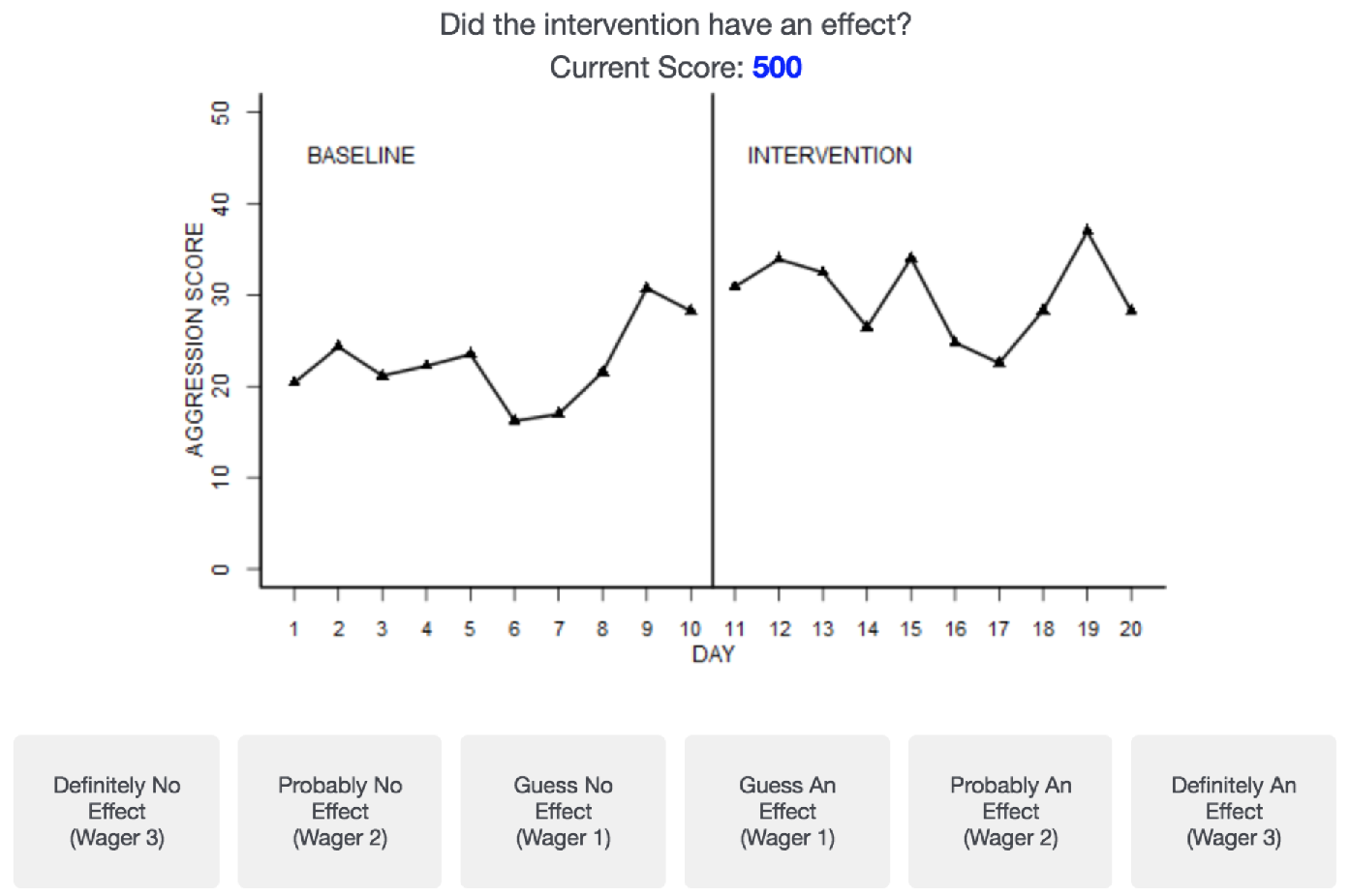
| Figure 2: An example trial that participants were shown during
instructions. Critical trials in the experiment had the same layout, but
without the current score shown. |
Next, to further assure understanding of the task and point system,
participants did 40 practice trials. During practice trials, the
current number of points (i.e., current score) was always visible. The
starting score was 250 and points could be earned or lost based on
participants’ wagers. Participants made decisions by selecting a button on
the Likert scale with the mouse, and then selecting the “next” button. On
practice trials, the subsequent screen continued to show the graph they
had just judged, but the correct answer (e.g., “Effect Present”) was shown
across the bottom of the screen in place of the Likert scale. The current
score was shown above the graph. Immediately above the current score, they
were shown how the decision had affected their score (raised or lowered
and by how much). There were an equal number of graphs (10) from each
condition during practice trials.
Next, participants completed 80 critical trials, with an equal number of
graphs (20) for each condition. Participants were not provided information
as to the number of critical trials, or the distribution of the types of
graphs. Order of trials was random for each participant. To mimic most
real-world circumstances, no feedback on accuracy, points earned, or point
totals appeared during the critical trials. Participants were informed that
they would still gain and lose points despite the absence of feedback. At
the end of the experiment, the screen revealed their final score.
3 Experiment 2 Method
3.1 Participants
Initially, 47 graduate students were recruited from the Teaching Behavior
Analysis mailing list at University of Houston, Downtown, with 46 from
U.S. institutions and one from a Northern Ireland institution. These
graduate students were primarily from programs in behavior analysis,
including both the experimental analysis of behavior and applied behavior
analysis. We chose this cohort because single-subject designs are prominent
in this area of psychology. One participant was excluded using the same
exclusion rules as before, leading to a final sample size of n =
46 (12 male). Nearly all participants (95.7%) had completed a course with
an emphasis on single-subject design, and the majority (71.7%) had used
single-subject design in their own research or projects. At the time of
the experiment, 41% of participants had a Master’s degree, and 7% a Ph.D.
Age ranged from 21 to 38 (M = 27.2, SD =
3.9). Participants were paid 5 cents (rather than 2 cents) per point, for a
total payment between $12.50 and $30.50. Graduate student status was
verified via online department directories when available, and when not
available, respondents were verified to have a university or college email
address at the institution with the graduate program that they reported to
be attending.
3.2 Procedure
There were three changes relative to the previous experiment. First, there
were extended demographic questions pertaining to experience with
single-subject designs. Second, after the instructions and examples, but
prior to the practice trials, participants were asked, “What percentage of
graphs do you expect to judge correctly (50% would be random guessing,
and 100% would be completely accurate)?” Third, after the experiment was
complete, they were asked to estimate their accuracy again.
4 Results (Experiments 1 and 2)
Analyses of graph judgment focus on the 80 critical graphs. First, for a
simplified overview, accuracy was analyzed by collapsing across confidence
levels. For example, if there was a treatment effect in the graph, any of
the three “…an Effect” responses were considered accurate. As shown in
Figure 3, accuracy declined when serial dependence was present, but only if
there was no treatment effect. In other words, serial dependence led to
Type I errors, but not Type II errors. In Experiment 1, a repeated
measures ANOVA showed a significant main effect of treatment
(F(1,49) = 33.1, p <. 001, ηp2 =.40), a
significant main effect of serial dependence (F(1,49) = 39.5,
p < .001, ηp2 =.45), and a significant interaction
effect between treatment effect and serial dependence (F(1,49) =
56.7, p < .001, ηp2 =.54). When there was a
treatment effect, there was no significant effect of serial dependence, as
shown by Tukey’s HSD (p = .81). In contrast, when there was no
treatment effect, the presence of serial dependence led to a significant
decline in accuracy (p < .001).
In Experiment 2, despite recruiting participants with relevant training,
the results were very similar (see Figure 3, right). Both main effects and
the interaction were significant (all ps < .001,
ηp2 = .34, .49, and .50, respectively). When there was a treatment
effect, there was no significant effect of serial dependence (p =
.59). In contrast, when there was no treatment effect, the presence of
serial dependence led to a significant decline in accuracy (p
< .001).
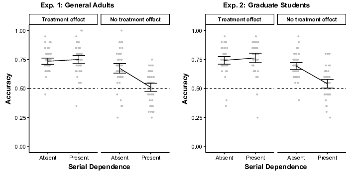
| Figure 3: Accuracy in each condition collapsed across confidence
levels. Dots show individual participants. Brackets show 95% CIs of the
mean. |
Next, Type I errors (decisions that a treatment effect existed even when it
did not) were analyzed separately at three levels of confidence. In
Experiment 1 (see Figure 4, left panel), Type I errors increased when
serial dependence was present, and this pattern occurred regardless of the
level of confidence. When confidence was “Guess An Effect” or higher,
Type I error rates significantly increased from the Serial Dependence
Absent (M = .33) to Present (M = .49) conditions
(t(49) = 9.19, p < .001, d = 1.30).
This pattern still held when counting only “Probably An Effect” or higher
(Ms = .20 and .34; t(49) = 8.38, p <
.001, d = 1.19), and when counting only the highest level of
confidence, “Definitely An Effect” (Ms = .09 and .20;
t(49) = 7.64, p < .001, d = 1.08).
Experiment 2 showed similar results (all ps <.001), with
d = 1.20, 1.38, and 1.04, moving from left to right in the right
panel of Figure 4.
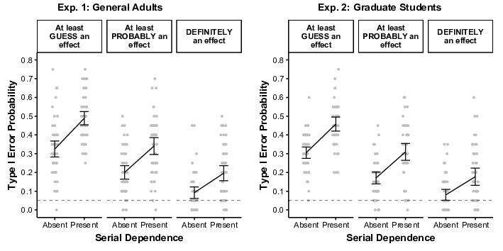
| Figure 4: Type I Error rates as a function of confidence level
(upper boxes) and serial dependence. Dots show individual participants.
Brackets show 95% CIs of the mean. Dashed lines show the customarily
desired Type I error rate of .05. |
Random number generators will sometimes produce graphs that coincidentally
have a significant treatment effect even where none exists in the
population (see Fisher et al., 2003). To determine the prevalence of such
coincidences, we applied a formal hypothesis test known to be robust to
serial dependence even in small samples of data. Specifically, we
analyzed graphs with a parametric bootstrap of the null hypothesis, with
the sample autocorrelation used for the simulation of 10,000 bootstrap
replicates per graph (see Borckardt et al., 2008, for details and evidence
of robustness). This analysis yielded a Type I error rate of .10
regardless of serial dependence being present or absent (2 graphs out of
20 for each), suggesting that the different judgment results for those
conditions was not due simply to a coincidence of graph generation. To
verify that the population generating equations behaved properly, we also
conducted this analysis with 10,000 runs of Equations 1–2 with no
treatment effect, once with serial dependence present and once with it
absent. This resulted in estimated Type I error rates below .05
regardless of serial dependence (.046 when present, .043 when absent),
providing further verification that informal judgment Type I error rates
were not artifacts of the generating equations.
Next, we considered the possibility that inflated Type I errors amidst
serial dependence were consistent with a simple heuristic: comparing the
absolute difference between the average baseline and average intervention
data points. To consider this in the long-run, we used Equations 1–2 to
simulate 100,000 time-series for each of the serial dependence conditions,
always with the null hypothesis true (no treatment effect). As expected,
the average raw difference between baseline and intervention periods was
.00, but importantly, the result was more variable when serial dependence
was present (SD=3.0) than when it was absent (SD=2.2).
This heightened variability led to significantly higher absolute
differences. Specifically, when serial dependence was present, the
intervention period was on average 2.4 points higher or lower than
baseline, as compared to only 1.8 points when serial dependence was
absent, Welch’s t(184,282)=85.7, p
< .001. When considering only the 20 critical stimuli in each
condition, there was a similar trend, with an absolute difference of 2.6
when serial dependence was present versus 1.8 when it was absent, though
this was not significant in this smaller sample, Welch’s
t(34.8) =1.54, p=.13. Overall, inflated Type I errors
amidst serial dependence would be expected if participants were relying on
an absolute difference heuristic.
Performance across all possible confidence criteria was analyzed via
Receiver Operating Characteristics (ROCs; Peterson & Birdsall, 1953; Swets
et al., 2000). ROCs also allow estimation of both the ability to
discriminate between treatment and no-treatment effects, and the bias
toward deciding that there was a treatment effect. As shown in Figure 5,
ROCs indicated better performance (closer to the upper left corner) when
serial dependence was absent than when it was present. Each dot represents
a different confidence criterion. For example, on the dashed line, the
left-most dot represents only the highest confidence criterion: “Definitely
an Effect.” The second dot from the left represents a more relaxed
confidence criterion: “Definitely an Effect” or “Probably an Effect”. The
more relaxed confidence criterion produces more power, but also more Type I
errors. Exactly five criteria (dots) are possible here, one for each
location in-between the six response options.
Participants’ discrimination between treatment effect and no treatment
effect graphs was measured by the area under the curve (AUC; specifically,
Ag in MacMillan & Creelman, 2005). In Experiment
1, AUC was significantly larger when serial dependence was absent
(M = .75) than when it was present (.67), suggesting that serial
dependence made it harder to discriminate treatment effects from no
treatment effects (t(49) = 7.34, p < .001,
d = 1.04). Similar results occurred in Experiment 2 (Ms
= .77 and .69; t(45)=6.85, p < .001, d
= 1.01). Bias to decide that there was an effect was measured by
Kornbrot’s (2006) nonparametric ln(βκ′) on the threshold
between “Guess No Effect” and “Guess An Effect.” The higher the
ln(βκ′), the more bias there is to decide that there is
an effect in the graph. In Experiment 1, participants were significantly
more biased toward selecting a button with “…An Effect” when serial
dependence was present (M=.75) than when it was absent (.19;
t(49) = 7.39, p < .001, d = 1.04).
Experiment 2 produced a similar pattern (Ms = .68 and .14;
t(45) = 6.71, p < .001, d = .99).
Overall, ROCs suggested that serial dependence affected performance in two
ways, first by reducing discriminability between treatment and no treatment
effects, and second by increasing bias toward deciding that there was a
treatment effect.
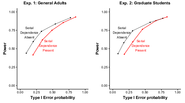
| Figure 5: Receiver Operating Characteristics (ROCs) closer to
the upper left corner indicate better discriminability. Specifically,
ROCs here show participants’ mean probabilities of correctly declaring a
treatment effect (Power) and incorrectly declaring a treatment effect
(Type I Error) across all confidence criteria. |
The effect of serial dependence on discriminability can also be seen in the
proportion of responses to each individual confidence category, as shown
in Figure 6. When a treatment effect was in the graph, participants
rarely chose “...No Effect” confidence categories, and more often chose
“...An Effect” categories, as expected. The reverse pattern appeared when
there was no treatment effect in the graph, or at least when serial
dependence was absent (black dashed lines on bottom panels). However,
when there was no treatment effect and serial dependence was
present (red lines on bottom panels), responses were spread more
evenly across all categories, consistent with the impaired
discriminability in that condition.
In Experiment 2, participants also made metacognitive judgments.
Immediately after the instructions and examples, participants
significantly overestimated the accuracy that they would achieve on the
task, predicting that they would achieve on average .80 proportion
accurate while achieving only .69 (t(45)=8.84, p
< .001, d = 1.30). After the experiment was finished,
participants significantly underestimated their actual accuracy,
estimating on average .65 accuracy (t(45)=2.79, p =
.008, d = .41). Actual accuracy was positively correlated with
estimated accuracy, both at the beginning (r = .43, p =
.003) and end (r = .37, p = .011) of the experiment.
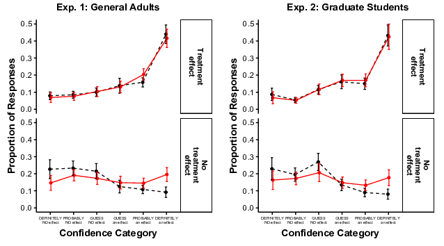
| Figure 6: Proportion of responses in each confidence category as
a function of treatment effect and serial dependence. Brackets show 95%
CIs of the mean. |
5 General Discussion
In both experiments, serial dependence increased the Type I error rate of
informal judgments of graphs, as measured by decisions that there was an
effect even when no effect existed in the population. This pattern
replicates the general finding of Matyas and Greenwood (1990), and it is
difficult to discount these findings using criticisms leveled at the
earlier work. The inflated Type I error rate occurred for most
participants, and in both guesses and highly confident responses. Because
Type I error inflation occurred even with high confidence responses, it is
unlikely that offering a zero-wager or “pass” option would eliminate this
pattern (see Dhar & Simonson, 2003). Furthermore, Type I error inflation
occurred even though each no-treatment condition was represented by 20
random graphs rather than just 1. It occurred even with a corrected
data-generating equation, and even though the proportion of response
options for no treatment effect (.5) was equal to the proportion of trials
with no treatment effect (.5).
When serial dependence was present, the Type I error rate was inflated
relative to the typical statistical standard of 5%, and even relative to
a statistical test of the graphs themselves (10%). In contrast to
earlier work, though, the Type I error rate never exceeded 49% by any
measure, let alone reached the 84% observed in Matyas and Greenwood
(1990), or the 61% observed in classic simulations of p-hacking (Simmons
et al., 2011). The more tempered Type I error rates observed here might be
the result of addressing methodological concerns. Of course, this pattern
provides little comfort, as Type I errors rates still exceeded the
customary 5% standard.
All participants were paid based on performance, so it is unlikely that the
elevated error rates were due to lack of motivation. They are also
unlikely due to simple misunderstandings, as all participants received
extensive training with feedback before beginning the experiment.
Furthermore, most graduate students in Experiment 2 had first-hand
experience using single-subject designs. Nevertheless, their performance
was not markedly different from that of a general adult sample. Indeed,
others have found little or no impact of single-subject design experience
on graph judgment (Harbst et al., 1991; Richards et al., 1997), though
such disappointing findings are not universal (see Kratochwill et al.,
2014). In our experiments, it is possible that any effects of graduate
training were overshadowed by the extensive task-specific practice with
feedback that all our participants received. It has been suggested that
such practice is crucial, as real-life rarely provides such clear feedback
(Parsonson & Baer, 1992). Indeed, prior to this practice, most graduate
students overestimated their own abilities for this task. The practice
and the remainder of the experiment were sobering, as by the end of the
experiment, participants tended to slightly underestimate their
performance.
Overconfidence sometimes disappears when participants make metacognitive
judgments about trials in aggregate at the end of an experiment
(Gigerenzer et al., 1991). One reason that could have happened here is
that participants were relying on different cues with different validities
at the beginning versus at the end of the experiment. At the beginning of
the experiment, graduate students’ metacognition probably
relied on cues that had only modest validity. For example, prior to the
experiment, they may have noticed when their belief in a treatment effect
agreed with the belief expressed by textbook authors, their mentors, or
fellow students when informally judging graphs, and used this agreement as
a cue to assess their own performance. The experiment, though, provided a
cue with perfect validity – feedback about the correct answer – at least
for the practice trials. By the end of this experiment, participants
could rely on memory for practice trial feedback to assess their own
performance.
As indicated by the ROCs, serial dependence affected performance in at
least two manners. First, serial dependence made it more difficult for
participants to distinguish between treatment and no-treatment conditions.
This difficulty might have occurred because the data points on the graph
(yt) become more variable as the
autoregressive parameter (a) gets farther from 0. Second, serial
dependence created a bias toward more “treatment” responses. This bias
could have occurred because, when serial dependence is present, one
especially large error value (et) can
affect several data points that follow it, producing the appearance of a
lasting change (Matyas & Greenwood, 1997). Relatedly, serial dependence
tends to create larger absolute differences between baseline and
intervention periods. So, the pattern of results is consistent with a
heuristic whereby people attempt to mentally subtract the mean of the
baseline period from the mean of the intervention period, and if the
absolute difference is large enough, decide that a treatment effect has
occurred. Such a heuristic would be useful for judging intervention
effectiveness, but it also makes one vulnerable to illusions of
intervention effectiveness, particularly if one uses the same threshold
regardless of the degree of dependence. Of course, it is unlikely that
this heuristic is the only heuristic that people rely upon. Disentangling
heuristics for statistical judgment is challenging because many plausible
heuristics make predictions that are strongly correlated (e.g., Obrecht et
al., 2007; Soo & Rottman, 2018, 2020). For example, participants could
adjust for variability in the data, treating absolute differences as more
meaningful when variability is smaller. Such an approach would be an
informal estimate of the absolute standardized difference (and
also an informal estimate of the absolute point-biserial correlation,
which is just a multiple of the absolute standardized difference). In our
stimuli, the absolute standardized difference is almost perfectly
correlated with the absolute raw difference, preventing us from
disentangling the two.
The current work differs from classic examples of illusory correlation
(e.g., Chapman & Chapman, 1969) where the judged datapoints were
typically independent (e.g., judging independent people). The results here
show that dependent observations across time can cause changes in
judgment, perhaps because an error term that applies to multiple time
points can be misattributed to a real change even where none exists. This
illusory correlation between the interruption and datapoint height was
observed here even in the absence of prior beliefs or expectations (c.f.,
Chapman & Chapman, 1969). Of course, such alternative causes of illusory
correlation could impact time series judgment as well, potentially
interacting with serial dependence. For example, a pattern produced by
serial dependence might be especially attended to when that pattern also
confirms the viewer’s expectations.
In a related finding, informal judgments for forecasting (extrapolating
into future parts of time-series data) are also prone to error, as they
are often less accurate than forecasts achieved by formal statistical
models (Carbone & Gorr, 1985). It is possible that informal forecasting
is also hampered by serial dependence. Serial dependence, at least when
positive, can make data appear to be smoother and more stable, even while
simultaneously creating more variability in the possible realizations of
time series patterns. So, ironically, informal forecasts might be most
certain when certainty is least warranted.
Unfortunately, serial dependence is a common attribute of time series data
(Harrington & Velicer, 2015; Shadish & Sullivan, 2011). Serial
dependence is what necessitates tools for time series beyond the typical
inferential statistics (e.g., t-tests, ANOVAs). Perhaps more troubling,
our experiments involved a rather minor form of dependence, a 1-lag
autoregressive coefficient of .3. Datasets that show stronger
dependencies may be more likely to lead to misattribution of error to real
patterns.
Conversely, it is likely that serial dependence is harmless in some
situations. If effect sizes are extremely large,
judgment should reach perfect performance, eliminating all types of errors.
Informal judgment seems sufficient, for example, to determine that the
American stock market dropped in the great crash of 1929. Additionally,
negative serial dependence produces high scores that are followed by low
scores, and vice-versa. It is unclear whether such alternating data
patterns would also bias respondents toward treatment effect decisions (see
Ximenes et al., 2009). Furthermore, dependencies could involve longer
lags, multiple lags, or seasonal effects. Considering the breadth of the
standard model for time series (Autoregressive Integrated Moving Average,
i.e., ARIMA), we examined just a simple case that is often used as a proxy
for potentially more complicated ones (see Harrop & Velicer, 1985).
We hope that our results are not oversimplified so as to malign informal
graph judgment in general. After all, we have relied on readers’ informal
graph judgment, in addition to formal statistical judgment, to evaluate
our data. However, interrupted time-series graphs may justify extra
caution, as they often involve serial dependence. Misjudgment of these
graphs could have substantial costs, particularly if illusory correlation
leads to illusory causation. Those who judge interrupted time-series
graphs might infer that certain events affect the stock market, public
health, individual patients, or other outcomes, even when they do not.
The risk of misjudgment could be mitigated by corroborating informal graph
judgment with formal statistical procedures (Bishara et al., 2021).
Of course, formal statistical procedures can also fail if they do not
accommodate the serial dependence in time-series data. Serial dependence
necessitates the use of special statistical models (e.g., ARIMA; Box et
al., 2015) rather than more typical ones that assume independent
observations (e.g., t-tests). Additionally, in small sample sizes – such
as the 20-observation graphs used here — typical time-series models often
fail to control Type I errors (Greenwood & Matyas, 1990) due to noisy
estimates of serial dependence. Such small sample situations also require
bootstrapping to prevent Type I error inflation (Borckardt et al., 2008;
Lin et al., 2016; McKean & Zhang, 2018;
McKnight et al., 2000; ). As daunting as these formal
statistical options may be, the alternative – informal judgment – can too
easily lead to “discovery” of patterns where none exist.
References
Baron, J. (2008). Thinking and deciding (4th
ed.). Cambridge University Press.
Bishara, A. J., Li, J., & Conley, C. (2021). Informal versus formal
judgment of statistical models: The case of normality assumptions.
Psychonomic Bulletin & Review. https://doi.org/10.3758/s13423-021-01879-z.
Borckardt, J. J., Nash, M. R., Murphy, M. D., Moore, M., Shaw, D., &
O’Neil, P. (2008). Clinical practice as natural
laboratory for psychotherapy research: A guide to case-based time-series
analysis. American Psychologist, 63(2), 77.
http://dx.doi.org/10.1037/0003-066X.63.2.77.
Box, G. E., Jenkins, G. M., Reinsel, G. C., & Ljung, G. M. (2015).
Time series analysis: forecasting and control
(5th ed.). John Wiley & Sons.
Brossart, D. F., Parker, R. I., Olson, E. A., & Mahadevan, L. (2006). The
relationship between visual analysis and five statistical analyses in a
simple AB single-case research design. Behavior Modification,
30(5), 531–563. https://doi.org/10.1177/0145445503261167.
Carbone, R., & Gorr, W. L. (1985). Accuracy of judgmental forecasting of
time series. Decision Sciences, 16(2), 153–160.
Chapman, L. J. (1967). Illusory correlation in observational report.
Journal of Verbal Learning and Verbal Behavior, 6(1), 151–155.
Chapman, L. J., & Chapman, J. P. (1969). Illusory correlation as an
obstacle to the use of valid psychodiagnostic signs. Journal of
Abnormal Psychology, 74(3), 271–280.
Clarke, R. D. (1946). An application of the Poisson distribution.
Journal of the Institute of Actuaries, 72(3), 481–481.
Dhar, R., & Simonson, I. (2003). The effect of forced choice on choice.
Journal of Marketing Research, 40(2), 146–160.
Fisher, W. W., Kelley, M. E., & Lomas, J. E. (2003). Visual aids and
structured criteria for improving visual inspection and interpretation of
single-case designs. Journal of Applied Behavior Analysis, 36,
387–406. https://doi.org/10.1901/jaba.2003.36-387.
Gigerenzer, G., Hoffrage, U., & Kleinbölting, H. (1991). Probabilistic
mental models: A Brunswikian theory of confidence. Psychological
Review, 98(4), 506.
Gilovich, T. (1991). How we know what isn’t so. Simon and
Schuster.
Greenwood, K. M., & Matyas, T. A. (1990). Problems with the application of
interrupted time series analysis for brief single-subject data.
Behavioral Assessment, 12, 355–370.
Hamilton, D. L., & Rose, T. L. (1980). Illusory correlation and the
maintenance of stereotypic beliefs. Journal of Personality and
Social Psychology, 39(5), 832–845.
Harbst, K. B., Ottenbacher, K. J., & Harris, S. R. (1991). Interrater
reliability of therapists’ judgments of graphed data.
Physical Therapy, 71, 107–115.
https://doi.org/10.1093/ptj/71.2.107.
Harrington, M., & Velicer, W. F. (2015). Comparing visual and statistical
analysis in single-case studies using published studies.
Multivariate Behavioral Research, 50, 162–183.
https://doi.org/10.1080/00273171.2014.973989.
Harrop, J. W., & Velicer, W. F. (1985). A comparison of alternative
approaches to the analysis of interrupted time-series.
Multivariate Behavioral Research, 20, 27–44.
https://doi.org/10.1207/s15327906mbr2001_2.
John, L. K., Loewenstein, G., & Prelec, D. (2012). Measuring the
prevalence of questionable research practices with incentives for truth
telling. Psychological Science, 23, 524–532.
https://doi.org/10.1177/0956797611430953.
Jones, R. R., Weinrott, M. R., & Vaught, R. S. (1978). Effects of serial
dependency on the agreement between visual and statistical inference.
Journal of Applied Behavior Analysis, 11, 277–283.
https://doi.org/10.1901/jaba.1978.11-277.
Kornbrot, D. E. (2006). Signal detection theory, the approach of choice:
Model-based and distribution-free measures and evaluation.
Perception & Psychophysics, 68(3), 393–414.
https://doi.org/10.3758/BF03193685.
Kratochwill, T. R., Levin, J. R., Horner, R. H., & Swoboda, C. M. (2014).
Visual analysis of single-case intervention research: Conceptual and
methodological issues. In T. R. Kratochwill & J. R Levin (Eds.),
Single-case intervention research: Methodological and statistical
advances (pp. 91–126). Washington, DC: American Psychological
Association. https://doi.org/10.1037/14376-004.
Lin, S. X., Morrison, L., Smith, P. W., Hargood, C., Weal, M., & Yardley,
L. (2016). Properties of bootstrap tests for N-of-1 studies.
British Journal of Mathematical and Statistical Psychology, 69,
276–290.
MacMillan, N. A., & Creelman, C. D., (2005). Detection theory: a
user’s guide. Lawrence Erlbaum Associates.
https://doi.org/10.4324/9781410611147.
Matyas, T. A., & Greenwood, K. M. (1990). Visual analysis of single-case
time series: Effects of variability, serial dependence, and magnitude of
intervention effects. Journal of Applied Behavior
Analysis, 23(3), 341–351.
https://doi.org/10.1901/jaba.1990.23-341.
Matyas, T. A., & Greenwood, K. M. (1997). Serial dependency in
single-case time series. In R. D. Franklin, D. B. Allison, and B. S.
Gorman (Eds.), Design and Analysis of Single-Case Research (pp.
215–244). Mahwah, NJ: L. Erlbaum Associates.
https://doi.org/10.4324/9781315806402.
McKean, J. W., & Zhang, S. (2018). DBfit: A double bootstrap method for
analyzing linear models with autoregressive errors. R package version 1.0.
https://CRAN.R-project.org/package=DBfit
McKnight, S. D., McKean, J. W., & Huitema, B. E. (2000). A double
bootstrap method to analyze linear models with autoregressive error terms.
Psychological Methods, 5, 87–101.
https://doi.org/10.1037/1082-989X.5.1.87.
National Centers for Environmental Information. (2020). Record of
Climatological Observations [Data set]. United States Department of
Commerce. Retrieved January 24, 2021, from
https://gis.ncdc.noaa.gov/maps/ncei/summaries/daily
Obrecht, N. A., Chapman, G. B., & Gelman, R. (2007). Intuitive t tests:
Lay use of statistical information. Psychonomic Bulletin &
Review, 14(6), 1147–1152.
Parsonson, B. S., & Baer, D. M. (1992). The visual analysis of data, and
current research into the stimuli controlling it. In T. R. Kratochwill &
J. R. Levin (Eds.), Single-Case Research Design and Analysis,
(pp. 15–39). Hillsdale, NJ: Lawrence Erlbaum Associates.
https://doi.org/10.4324/9781315725994.
Peterson, W. W., & Birdsall, T. G. (1953). The theory of signal
detectability. Technical Report No. 13. Engineering Research Institute,
University of Michigan. https://doi.org/10.1109/TIT.1954.1057460.
R Core Team (2018). R: A language and environment for statistical
computing. R Foundation for Statistical Computing, Vienna, Austria. URL
https://www.R-project.org/.
Richards, S. B., Taylor, R. L., & Ramasamy, R. (1997). Effects of subject
and rater characteristics on the accuracy of visual analysis of single
subject data. Psychology in the Schools, 34, 355–362.
https://doi.org/10.1002/(SICI)1520-6807(199710)34:4<355::AID-PITS7>3.0.CO;2-K.
Shadish, W. R., & Sullivan, K. J. (2011). Characteristics of single-case
designs used to assess intervention effects in 2008. Behavior
Research Methods, 43, 971–980.
https://doi.org/10.3758/s13428-011-0111-y.
Simmons, J. P., Nelson, L. D., & Simonsohn, U. (2011). False-positive
psychology: Undisclosed flexibility in data collection and analysis allows
presenting anything as significant. Psychological Science, 22,
1359–1366. https://doi.org/10.1177/0956797611417632.
Skinner, B. F. (1956). A case history in scientific method.
American Psychologist, 11, 221–233.
https://doi.org/10.1037/h0047662.
Smith, J. D. (2012). Single-case experimental designs: A systematic review
of published research and current standards. Psychological
Methods, 17(4), 510. https://doi.org/10.1037/a0029312.
Soo, K. W., & Rottman, B. M. (2018). Causal strength induction from time
series data. Journal of Experimental Psychology: General, 147,
485–513.
Soo, K. W., & Rottman, B. M. (2020). Distinguishing causation and
correlation: Causal learning from time-series graphs with trends.
Cognition, 195, 104079.
Swets, J. A., Dawes, R. M., & Monahan, J. (2000). Psychological science
can improve diagnostic decisions. Psychological Science in the
Public Interest, 1(1), 1–26.
https://doi.org/10.1111/1529-1006.001.
Vyse, S. A. (2013). Believing in magic: The psychology of
superstition-updated edition. Oxford University Press.
Xie, B., & Hayes, B. (2020, November 19–22) When are people sensitive to
information dependency in judgments under uncertainty [Poster]. Psychonomic
Society 61st Annual Meeting, virtual.
https://www.webcastregister.live/psychonomic2020annualmeeting.
Ximenes, V. M., Manolov, R., Solanas, A., & Quera, V. (2009). Factors
affecting visual inference in single-case designs. The Spanish
Journal of Psychology, 12, 823–832.
https://doi.org/10.1017/S1138741600002195.
Appendix: Proof that generating equations in previous work
created on-average differences between the periods before versus after
the interruption
From Matyas and Greenwood (1990, p. 343):
When there is no treatment effect, d = 0. Also, for clarity, relabeling e as et:
The long-run average is the expectation ( E). For example, with the first trial (t=1),
|
| |
E | ⎡
⎣ | y1 | ⎤
⎦ | = E | ⎡
⎣ | ay0+b+e1 | ⎤
⎦ | =a E[y0]+ E[b]+ E[e1]
|
|
(5) |
There is no trial 0, so the term with y0 drops out. Also, b is a constant, so E[b] = b. Because et is generated from a population with a mean of 0, E[et] = 0 for all t. This simplifies the average data point of trial 1:
For trial 2,
|
| |
E | ⎡
⎣ | y2 | ⎤
⎦ | = a E[y1]+ E[b]+ E[e2] = ab+b = | ⎛
⎝ | a+1 | ⎞
⎠ | b
|
|
(7) |
For trial 3,
|
| |
E | ⎡
⎣ | y3 | ⎤
⎦ | =a E[y2]+ E[b]+ E[e3] = a | ⎛
⎝ | a+1 | ⎞
⎠ | b+b = (a2+a+1)b
|
|
(8) |
More generally, for any trial,
|
E | ⎡
⎣ | yt | ⎤
⎦ | =(at−1+at−2+…+a0)b
(9) |
We need only show that the expectations differ before (t ≤ 10) versus after the interruption (t > 10) for at least one pair of trials. For simplicity, consider the average difference between the trials 11 and 1:
|
| |
E | ⎡
⎣ | y11−y1 | ⎤
⎦ | = | ⎛
⎝ | a10+a9+…+a1+a0 | ⎞
⎠ | b−b = | ⎛
⎝ | a10+a9+…+a1 | ⎞
⎠ | b
|
|
(10) |
The very first trial and the first trial after the interruption differ on average then, so long as a ≠ 0, a ≠ −1, and b ≠ 0. Although b was never explicitly defined in the text, the graphs (Matyas & Greenwood, 1990, p. 344) clearly indicate a value much larger than 0 (b ≈ 20). Importantly, a ≠ 0 only in the conditions with serial dependence. So, when there is serial dependence, the generating equation in Matyas and Greenwood creates differences before versus after the interruption even when there is no treatment effect (d = 0). Response options indicating these differences (options B-E) were coded as Type I errors. Thus, this problem could account for their elevated Type I error rates in conditions with serial dependence.
This document was translated from LATEX by
HEVEA.