Judgment and Decision Making, Vol. 15, No. 6, November 2020, pp. 939-958
Coherence of probability judgments from uncertain evidence: Does ACH help?Christopher W. Karvetski*
David R. Mandel#
|
Although the Analysis of Competing Hypotheses method (ACH) is a structured
analytic technique promoted in several intelligence communities for
improving the quality of probabilistic hypothesis testing, it has received
little empirical testing. Whereas previous evaluations have used numerical
evidence assumed to be perfectly accurate, in the present experiment we
tested the effectiveness of ACH using a judgment task that presented
participants with uncertain evidence varying in source reliability and
information credibility. Participants (N = 227) assigned
probabilities to two alternative hypotheses across six cases that
systematically varied case features. Across multiple tests of coherence,
the ACH group showed no advantage over a no-technique control group. Both
groups showed evidence of subadditivity, unreliability, and overly
conservative non-Bayesian judgments. The ACH group also showed
pseudo-diagnostic weighting of evidence. The findings do not support the
claim that ACH is effective at improving probabilistic judgment.
Keywords: probability judgment, Analysis of Competing Hypotheses, coherence, uncertainty, evidence
1 Introduction
Criminal investigators, intelligence analysts and other experts routinely
judge the probability of competing hypotheses using evidence of varying
quality and type. For example, human intelligence from informants can
provide valuable insight but also must be carefully evaluated in terms of
the source’s reliability and the credibility of the information provided,
a step formally know as information evaluation within the
intelligence cycle (Irwin & Mandel, 2019; Samet, 1975). The failure to
correctly evaluate these characteristics can lead to serious intelligence
errors. For instance, significant evidence that motivated the US-led 2003
invasion of Iraq was based on fabricated claims of the informant
code-named Curveball, who described working as a chemical
engineer in support of Iraq’s biological weapons program (Drogin & Goetz,
2005).
To improve the quality of intelligence assessments, the US intelligence
community advises analysts to use structured analytic techniques (SATs)
(e.g., Office of the Director of National Intelligence, 2015; US
Government, 2009). A prominent SAT designed to aid analysts in evaluating
multiple hypotheses on the basis of evidence of varying quality is the
Analysis of Competing Hypotheses (ACH), formulated by Central Intelligence
Agency (CIA) analyst Richards Heuer (Heuer, 1999; Heuer & Pherson, 2014).
ACH starts with generating a set of mutually exclusive and collectively
exhaustive hypotheses that are listed in columns of a matrix, whereas
items of evidence are listed in rows. The analyst evaluates the quality of
each item of evidence in terms of its (a) credibility and reliability and
(b) relevance, and then moves along each row and assesses the pairwise
consistency of each item of evidence with each hypothesis. The analyst
then aggregates the assessments into final inconsistency scores, which are
intended to enable the analyst to evaluate the relative likelihood of
the hypotheses, at least on an ordinal scale. Whether used independently
or by a group of analysts, ACH is typically implemented in a software tool
called PARC (Palo Alto Research Center, 2006), in which all inputs are
selected from standardized lists (e.g., “high”, “medium”, “low” for
credibility/reliability and relevance; “very inconsistent”,
“inconsistent”, “neutral/not applicable”, “consistent”, “very
inconsistent” for hypothesis-evidence consistency). PARC matches the
selected ratings to numeric values and uses these to calculate an
inconsistency score for each alternative hypothesis.
The attitude of the intelligence community towards SATs (and ACH, in
particular) has been that, although they may not be perfect aides to the
analyst’s unaccompanied reasoning processes, they are almost certain not
to do harm and probably do good (Heuer, 2005). However, as others have
noted (Dhami, Mandel, Mellers & Tetlock, 2015; Karvetski, Olson, Gantz & Cross, 2013; Mandel & Tetlock, 2018), this conclusion may be premature.
SATs usually involve multiple steps that are of questionable reliability
and validity, and this is true of ACH (Chang, Berdini, Mandel & Tetlock,
2018; Mandel, 2020). For instance, ACH does not give analysts guidance on
how to parse or chunk evidence, or how to treat evidence that is not
independent. For instance, Karvetski, Mandel and Irwin (2020) found that
ACH users tended to rate two perfectly correlated cue values as if they
were fully independent sources of evidence. Increasing the salience of the
information redundancy made the tendency to treat the evidence as
independent even stronger. This suggests that ACH encourages the use of a
simple “copy repeating patterns” heuristic that fully ignores
correlational structure in evidence. Similarly, ACH does not define what
consistency means or how it should be assessed. Some analysts might
interpret it as the probability of the evidence given the hypothesis,
while others might interpret it as the inverse probability. Others still
might regard it as a call for an intuitive judgment of how well the
evidence and hypothesis seem to match one another—namely, as a call for
the application of the representativeness heuristic, which has been
implicated in several cognitive biases (Kahneman & Tversky, 1972). This
imprecision of input terms may foster inter-analyst inconsistency or the
same analyst might exhibit inconsistency over time or even within a
specific case.
While ACH is promoted to mitigate confirmation bias — the search for (or
use of) evidence to support a preferred hypothesis (Nickerson, 1998) — the
technique may be susceptible to other biases that are present within
evidential evaluation processes. For example, the enhancement effect
implies that an increased perception of the degree to which the evidence
is compatible with three or more mutually exclusive and exhaustive
hypotheses can result in all hypotheses being judged as more likely than
possible (Rottenstreich & Tversky, 1997; Tversky & Koehler, 1994). This
implies the assigned hypothesis probabilities sum to more than one. Given
that ACH provides no check on additivity violations and does not even make
the probabilities of hypotheses explicit, it is unlikely to mitigate this
bias in evidence assessment.
Recent research on the effectiveness of ACH calls into question the
effectiveness of this method for mitigating biases and improving judgment
accuracy. Whitesmith (2019) found that ACH did not mitigate either
confirmation bias or serial-position effects on the interpretation of
evidence in reasoning about an intelligence analysis scenario (also see
Lehner, Adelman, Cheikes & Brown, 2008). Mandel, Karvetski and Dhami
(2018) found that intelligence analysts who were instructed to use ACH on
a probabilistic hypothesis-testing task were less coherent and
marginally less accurate in assigning probabilities to the hypotheses than
analysts in a control group who were not instructed to use any SAT.
Moreover, a subsequent examination of analysts’ information use from the
same experiment showed that analysts in the ACH condition were
less likely to use relevant base-rate information than analysts
in the control condition (Dhami, Belton & Mandel, 2019). In another
experiment, Karvetski et al. (2020) found that mock analysts who judged
the probabilities of alternative hypotheses before and after using ACH
were less coherent (i.e., violating complementarity and additivity
constraints on probabilities) and they did not significantly differ from
the control group in terms of accuracy. In fact, aggregated judgments were
more accurate before using ACH than after using it, and the benefit of
not using ACH increased with the size of the aggregate. As
intelligence communities in the US and elsewhere invest in research to
leverage the wisdom of crowds through mechanisms such as prediction
markets (e.g., see Stastny & Lehner, 2018; cf. Mandel, 2019), the
relative cost of using ACH versus other methods may be amplified.
The preceding research not only casts doubt on the efficacy of ACH, it also
challenges the claim that SATs, at worst, do not help. The studies by
Mandel et al. (2018), Dhami et al. (2019), and Karvetski et al. (2020)
show that use of ACH can make analysts’ probability judgments about
alternative hypotheses worse than if ACH were not used. However, skeptics
might counter that the aforementioned studies not only lack mundane
realism, they also differ from real-life analysis in ways that undermine
the external validity of the research. For instance, participants in
Mandel et al. (2018) and Karvetski et al. (2020) received statistical
evidence that was described as being perfectly accurate and precise and
that was communicated using numeric probabilities, much as in earlier
experiments on probabilistic hypothesis testing (e.g., Slowiaczek,
Klayman, Sherman & Skov, 1992; Villejoubert & Mandel 2002). These
features enabled unambiguous scoring of accuracy using probabilistic truth
criteria, but they sacrifice mundane realism and perhaps external
validity as well. Therefore, such studies should be complemented by research that represents evidence more closely to how it often appears in
real-life investigations.
1.1 The Present Research
The aim of the present research was to provide a more externally valid test
of ACH. As in prior studies on ACH (e.g., Mandel et al., 2018; Karvetski,
2020), participants were asked to assign probabilities to alternative
hypotheses. However, to improve the external validity of tests of ACH, we
presented evidence (based on a hypothetical suspect’s criminal record)
with probabilities that were imprecisely communicated using linguistic
terms such as likely, much as an analyst would encounter in the
everyday intelligence practice (Barnes, 2016; Ho, Budescu, Dhami, &
Mandel, 2015; Mandel, 2015a). In each of six cases, we also presented
evidence from two human sources claiming to know the suspect. This
evidence was coded in terms of the source’s reliability and the
credibility of the information, following the Admiralty coding system
widely used in the evaluation step of the analysis stage within the
intelligence cycle (Irwin & Mandel, 2019; Samet, 1975). Prior to
receiving case-specific information, participants were asked to translate
the verbal probabilities and alphanumeric source reliability/information
credibility values used in the cases into their own probabilistic
interpretation of the evidence.
Although we have foregone the ability to directly assess ACH’s
effectiveness on correspondence criteria (i.e., accuracy) in this research, using the participants’ own probabilistic interpretation of the
evidence allows us to assess the effect of ACH on multiple coherence
criteria. Coherence criteria gauge the extent to which judges agree with
normative constraints on judgment or decisions or are otherwise internally
consistent (Hammond, 2000). As such, coherence criteria are fundamental to
sound reasoning, which the intelligence community views as a pillar of
analytic integrity (Office of the Director of National Intelligence,
2015). Coherence metrics have been shown to covary with correspondence
metrics such as accuracy in forecasting (Mellers, Baker, Chen, Mandel &
Tetlock, 2017). Several studies also show that judgment accuracy can be
improved by exploiting individual differences in coherence (Fan, Budescu,
Mandel & Himmelstein, 2019; Karvetski, Olson, Mandel & Twardy, 2013;
Mandel et al., 2018; Wang, Kulkarni & Poor, 2011). Therefore, performance
on coherence criteria can provide at least indirect evidence of how likely
a method such as ACH is to improve accuracy.
As in some earlier research (Dhami et al., 2019; Mandel et al., 2018), the
present research compared the performance of individuals using ACH to a
control condition in which participants judged probabilities without
instruction to use any SAT. The present experiment explored a fuller set of coherence metrics than in previous studies. A first test of
coherence examined the consistency between posterior probability judgments
and choice. Mandel (2015b) found that when intelligence analysts were
asked to judge the posterior probabilities of binary complements and
subsequently asked to make a binary choice regarding which hypothesis was
correct, only 53% chose the alternative with the higher probability
across all eight problems. This proportion substantially increased to 83%
after brief training in Bayesian reasoning using natural sampling trees
similar to protocols used in other studies (e.g., Sedlmeier & Gigerenzer,
2001). Dhami et al. (2019) further found that analysts who used ACH were
less likely than control analysts to show consistency between their final
conclusions and the penultimate judgments. However, that analysis was
based on a small sample. In the present research, which used a much larger
sample of participants, we also studied the consistency between
probabilities assigned to binary complements and whether participants
selected the alternative with the higher probability in their binary
choices. If ACH improves the quality of reasoning, then we might expect
greater consistency between judgment and choice in the ACH condition than
in the control group.
As a second test of coherence, we examined how reliable participants were
in their probability judgments across cases that had isomorphic evidence
configurations. In the present research, the six cases we used were
comprised of three isomorphic pairs of cases (i.e., surface
characteristics were switched but the cases had the same structure). If
ACH is effective at mitigating unreliability due to so-called
“unstructured reasoning,” we should observe greater reliability (i.e.,
within-pair consistency) among participants using ACH than among those in
the control group.
Several studies show that people violate the additivity constraint in
probability judgment, for example by providing subadditive judgments of
probabilities among mutually exclusive and exhaustive hypotheses that sum
to more than unity (Ayton, 1997; Mandel, 2005, 2008; Tversky & Koehler,
1994). In an exercise that involved having analysts assess the likelihood
of four competing hypotheses in a single case using diagnostic cues of
various levels of support, Mandel et al. (2018) found that compared to a
control condition, ACH led to greater subadditivity (i.e., the sum of four
mutually exclusive and exhaustive hypotheses exceeded 1). Karvetski et al.
(2020) further confirmed that ACH increased within-subject incoherence
using a task that involved judging the probabilities of three mutually
exclusive and collectively exhaustive hypotheses within a single case. In
the present research, we tested the effect of ACH on additivity violations
from the complementarity rule, which requires that P(x)
+ P(¬x) = 1. This provided a third test of
coherence.
Some studies evaluating adherence to the complementarity rule have found
additivity (Tversky & Fox, 1995; Tversky & Koehler, 1994; Wallsten, Budescu & Zwick, 1993), while others have found superadditivity (Macchi, Osherson &
Krantz, 1999, Mandel, 2005, 2015b), or a varying pattern of either
superadditivity and subadditivity (Idson, Krantz, Osherson & Bonini,
2001; Villejoubert & Mandel, 2002) or additivity and subadditivity (Dhami
& Mandel, 2013). It appears that the direction of complementarity
violations is influenced by the totality of evidential support for the
hypotheses. For instance, Idson et al. (2001) found that if participants
had little knowledge to draw upon, judgments were superadditive, whereas
if participants had greater knowledge, judgments were subadditive. In a
related vein, Villejoubert and Mandel attributed the direction of bias
from complementarity to the inverse fallacy, the tendency to confuse
posterior probabilities with their inverse, diagnostic probabilities. They
found that when the sum of the diagnostic probabilities was less than
unity, P(D|H1) + P(D|H2) <
1, posterior probabilities were superadditive, P(H1|D) +
P(H2|D) < 1. However, when the sum of the
diagnostic probabilities was greater than unity, P(D|H1)
+ P(D|H2) > 1, posterior probabilities were
subadditive, P(H1|D) + P(H2|D)
> 1. The present research includes multiple case scenarios
that varied the level of total evidential support, thus allowing further
tests of whether complementarity violations can be explained by
characteristics of evidence. We hypothesized that as total evidential
support increases, the total probability assigned to complementary
hypotheses will also increase, inducing subadditivity of probability
estimates.
As noted earlier, we elicit for every participant a probabilistic
interpretation of each uncertainty term. We calculated
participant-specific Bayesian posterior probabilities using these
estimates. This allowed us to analyze the coherence in a fourth manner:
namely, as agreement in the most likely hypothesis and the absolute
deviation between the participant’s elicited posterior probabilities and
those computed using Bayes theorem from their preceding translation
estimates. In addition to testing whether ACH improved consistency, we
tested whether there was evidence of conservatism (Edwards, 1968; Phillips
& Edwards, 1966)—namely, insufficient belief revision in light of the
evidence.
Finally, as a fifth test of coherence, we examined how participants in the
ACH condition weighed evidence. Lehner et al. (2008) found that
non-diagnostic evidence was often assigned non-neutral consistency scores,
indicating a form of pseudo-diagnosticity in consistency judgments, which
the authors called projection error. The proportion of such
errors did not differ between participants trained in and using ACH and
those who were neither trained in nor asked to use ACH. Lehner et al.’s
study, however, was statistically underpowered, having only 24
participants assigned to four conditions. Therefore, their findings, both
those found to be significant and those found to be nonsignificant, are of
questionable replicability and must be interpreted cautiously. In the
present research, we examined a related issue; namely, whether
non-diagnostic evidence equally favoring two alternative hypotheses would
be accordingly rated with an equal degree of consistency in ACH or,
alternatively, whether such non-diagnostic evidence would be rated in a
manner favoring one hypothesis over the other. Specifically, we tested the
hypothesis that participants using ACH will assign more positive
consistency ratings to the hypothesis suggested to be true by the
evidential claim if the probability of truth were disregarded. For
example, assuming x and ¬x as binary
complements, for an evidence claim that there is a 50% chance that
x is true, it would be appropriate for x and
¬x to be assigned equal consistency ratings in ACH. A
strict normative constraint might go even further, requiring that analysts
assign both hypotheses a neutral rating. However, on the basis of
research on framing effects, which shows that what is explicated in a
statement has more impact on judgment than what is logically implied
(Mandel, 2008; Tombu & Mandel, 2015), we expected that the hypothesis
explicitly matched to truth in the claim would receive a more positive
rating.
2 Method
2.1 Participants
Participants (N = 227) were recruited using the online
crowdsourcing service Qualtrics Panels and were required to (a) be at
least 18 years of age, (b) be fluent in English, (c) be a Canadian
citizen, (d) possess a Bachelor’s or higher degree, and (e) complete the
experiment on a computer (i.e., smartphones were prohibited). The mean age
was 40.7 years (SD = 11.9) and 26.4% were male.
2.2 Experimental design
The experiment used a one-factor (Method) between-subjects design in which
participants were randomly assigned to the ACH condition or to the control
condition. In the ACH condition, participants used the ACH method as
implemented in the PARC tool (PARC, 2006), whereas in the control
condition, participants were not required to use a SAT.
2.3 Procedure
The data were collected as part of a larger online survey. Participants
first read the consent form and provided they consented, they were first
asked to answer ten general knowledge questions for an unrelated study.
The next task was the primary one relevant to the present research, which
is described in detail below1. Following this task, participants completed
other tasks that were not related to the aims of the present research,
following which demographic information was collected and participants
were debriefed.
In the primary task, participants were asked to imagine that they were
hired as an analyst for a “Federal Law Enforcement Agency” whose mission
was to help local law enforcement agencies crack down on gang activity
within their respective locales. In particular, participants were told
they would be investigating multiple graffiti crime cases, each of which
concerned a single suspect, and that investigated activity within each
standalone case could be “either gang-related or else the act of a street
artist with no gang affiliation”, and that their task was “sorting through
each scenario provided by the local law enforcement centres, [with the
objective of providing] a probabilistic assessment concerning whether the
graffiti activity is gang-related or the work of a street artist.” Both
statements implied these two outcomes of gang member (GM) or
street artist (SA) as mutually exclusive and collectively
exhaustive hypotheses.
| Table 1: Prompts for probability equivalents
(Pe) for uncertainty terms. |
Elicited Judgment |
Assessed Question |
PHL | Assume a background check reveals that it is highly likely that a
suspect belongs to a certain category (e.g., gang member or street
artist). What is the probability that the suspect is in fact a member of
the described category? |
PL | Assume a background check reveals that it is likely that a suspect
belongs to a certain category (e.g., gang member or street artist). What
is the probability that the suspect is in fact a member of the described
category? |
PA1 | Let’s say an informant’s reliability is
assigned an A (completely reliable) and the credibility of the
informant’s information is assigned a 1 (completely
credible). If this informant were to make a claim about a suspect on the
basis of the information he or she provided, what is the probability that
the claim is accurate? |
PC3 | Let’s say an informant’s reliability is
assigned a C (fairly reliable) and the credibility of the
informant’s information is assigned a 3 (possibly true).
If this informant were to make a claim about a suspect on the basis of the
information he or she provided, what is the probability that the claim is
accurate? |
PF3 | Let’s say an informant’s reliability is
assigned an F (reliability cannot be judged) and the credibility of the
informant’s information is assigned a 3 (possibly true).
If this informant were to make a claim about a suspect on the basis of the
information he or she provided, what is the probability that the claim is
accurate? |
Prior to encountering any of the cases, participants provided an initial
set of five judgments that addressed the questions shown in Table 1, where
participants entered probabilities using a slider-bar that ranged from 0
to 1 with increments of 0.01. We denote each judgment generically as
Pe with e ∈ E
={HL, L, A1, C3, F3}. These judgments established participant-specific probability equivalents for the
verbal uncertainty terms that described evidence in the subsequent cases.
The first two questions elicited judgments
PHL and
PL, respectively, and addressed the two
verbal uncertainty terms of highly likely and likely.
These questions were presented first in randomized order. The
remaining three questions elicited judgments for three source reliability
and information credibility combinations
(PA1,
PC3, and
PF3) that were taken from the rating
system used in NATO’s Allied Intelligence Doctrine (NATO, 2015; see also
Irwin & Mandel, 2019; Samet, 1975). These questions were also presented
in randomized order, and the full rating scale (see bottom of Figure 1)
was presented above these questions for reference.
2.3.1 Control condition
After providing inputs for the questions in Table 1, participants in the
control condition saw an overview slide describing the format of each
case, but they received no additional instruction on how to analyze the
cases before encountering the six cases (which are described in the next
section). Case order was randomized per participant. Each case featured a
case description including a local (generic) gang name with which the
individual of the case was suspected of being affiliated, along with three
items of evidence. Figure 1 displays an example case presented to
participants. The first item of evidence within each case was a background
check conducted on the suspect that described which of the two hypotheses
was more likely from the findings (street artist in the example
of Figure 1), as well as a description of law enforcement’s subjective probability of that hypothesis being true (likely in the
example). The other two items of evidence within each case corresponded to
the testimony and assessment of two independent informants, where each
informant’s testimony and assessment showed three components of
information: (a) the informant’s claim, (b) a rating of the informant’s
source reliability, and (c) a rating of the credibility of the
information. For the case in Figure 1, Informant 1 is rated F3
and describes the suspect as a street artist. Informant 2, on the other
hand, is rated A1 and describes the suspect as a gang member.
Also, participants (in both conditions) were told to “Assume that the
informants cannot access the background check information and the
informants have had no communication with one another. More generally,
assume the three items of evidence are independent of one another.
Further, assume that the cases are independent of one another.”
For each case, participants in the control condition answered the following
two questions:
-
What is the probability that the suspect in the case below is a gang
member?
- What is the probability that the suspect in the case below is a
street artist?
Case file details for suspectLocal Gang: ALPHITES
Evidence item 1
Background check on suspect: Given the background check information on
suspect (before informants calling in) law enforcement believes it
is likely the suspect is a street artist.
Evidence item 2
Informant 1 Information: Informant 1 claims suspect is a street artist.
Reliability of Informant 1: (F) reliability cannot be judged.
Credibility of Informant 1’s information: (3) possibly true.
Evidence item 3
Informant 2 Information: Informant 2 claims suspect is a gang member.
Reliability of Informant 2: (A) completely reliable.
Credibility of Informant 2’s information: (1) completely credible.
Source Reliability and Information Index
| Source Reliability | Information Credibility |
| A | Completely reliable | 1 | Completely credible |
| B | Usually reliable | 2 | Probably true |
| C | Fairly reliable | 3 | Possibly true |
| D | Not usually reliable | 4 | Doubtful |
| E | Unreliable | 5 | Improbable |
| F | Reliability cannot be judged | 6 | Truth cannot be judged |
| Figure 1: Example case from the judgment task. |
The two elicited questions appeared on separate pages, with ordering
counterbalanced, and with the value entered using a slider that ranged
from 0 to 1, with increments of 0.01. The full case image (e.g., Figure 1)
was displayed below each question, and there was no requirement for the
two probabilities to sum to 1, nor a reference made to the relevance of
the complementarity constraint.2 Participants in the control
condition were then asked, “Given all the information presented in this
case, what will you recommend to your supervisor as the classification for
this suspect?” The participants submitted their final recommendation that
the suspect be classified as either a street artist or a gang member by
clicking on one of two selection buttons labelled “GANG MEMBER” or “STREET
ARTIST”. The buttons for the final recommendation appeared on the
same-screen with counter-balanced placement of which button was first, and
again the entire case file image was presented below the buttons. After
submitting the discrete recommendation for a suspect in a case,
participants in the control condition would then move the next case and
repeat the same assessment, until all six cases were completed.
Referring to the case details below, rate the source reliability and
information credibility of the three items of evidence on
the high (H), medium (M), or low (L) scale described earlier.
The source reliability and information credibility of the first item of
evidence (background check) is:
M
The source reliability and information credibility of the second item of
evidence (Informant 1) is:
L
The source reliability and information credibility of the third item of
evidence (Informant 2) is:
H
Case file details for suspect
Local Gang: ALPHITES
Evidence item 1
Background check on suspect: Given the background check information on
suspect (before informants calling in) law enforcement believes it
is likely the suspect is a street artist.
Evidence item 2
Informant 1 Information: Informant 1 claims suspect is a street artist.
Reliability of Informant 1: (F) reliability cannot be judged.
Credibility of Informant 1’s information: (3) possibly true.
Evidence item 3
Informant 2 Information: Informant 2 claims suspect is a gang member.
Reliability of Informant 2: (A) completely reliable.
Credibility of Informant 2’s information: (1) completely credible.
Source Reliability and Information Index
| Source Reliability | Information Credibility |
| A | Completely reliable | 1 | Completely credible |
| B | Usually reliable | 2 | Probably true |
| C | Fairly reliable | 3 | Possibly true |
| D | Not usually reliable | 4 | Doubtful |
| E | Unreliable | 5 | Improbable |
| F | Reliability cannot be judged | 6 | Truth cannot be judged |
| Figure 2: Example of Step 1 in the ACH process as implemented in the
experiment. |
2.3.2 ACH condition
After providing inputs for the questions in Table 1, participants in the
ACH condition were presented with an overview slide describing the format
of each case (as in the control condition). In contrast to the control
condition, participants were also given a one-slide overview on the ACH
procedure and were told they would be required to use the method in
evaluating the cases, with further instructions embedded within the
exercise. The ACH participants then encountered the same six cases
presented to the control participants, once again with case order
randomized per participant. For each case, the ACH participants went
through an ACH assessment procedure within Qualtrics that emulated ACH as
implemented in the PARC tool. For each case, participants completed the
following ACH assessment procedure:
-
Provide assessments of the source reliability and information
credibility as high (H), medium (M), or low (L) from a dropdown menu for
each of the three items of evidence.
- Provide assessments of the relevance as high (H), medium
(M), or low (L) from a dropdown menu for each of the three items of
evidence.
- Populate matrix cells (6 inputs total) with ratings of the
consistency between each item of evidence and each hypothesis, which
ranged from very inconsistent (II), inconsistent (I), neutral/not
applicable (N), consistent (C), or very consistent (CC). The qualitative
ratings had accompanying inconsistency scores.
- Sum the inconsistency scores for each of the two hypotheses, and
select the summation value from a dropdown menu in order to generate a
final inconsistency score for each hypothesis.
- Use the final inconsistency scores and provide probabilities that the
suspect in each case is a gang member or a street artist. Then provide a
final recommendation that the suspect be classified as either a street
artist or a gang member.
The ratings you just provided for source reliability/information
credibility and relevance are shown in brackets with each evidence item in
the tables below if you need to reference them. For this next step, please
fill in the consistency/inconsistency inputs below using the dropdown
menus. For each input, ask yourself if the evidence of the row is
consistent with the hypothesis at the top of the column (e.g., is the
background check consistent with the gang member hypothesis?). If the
answer is "Yes," use a consistency score to show that the attribute is
consistent (C) or very consistent (CC) with the hypothesis. If the answer
is "No," mark it as inconsistent (I) or very inconsistent (II). An
attribute may also be marked as neutral or not applicable to some
hypotheses (N). Please note that the numeric scores that show up in the
dropdown menu next to each rating are used in the next step.
| | H1 GANG MEMBER | H2 STREET ARTIST |
Evidence: Background check reports likely the suspect is a street artist | | |
[Recall your previous assessment for this item of evidence:
-
Source Reliability/Info. Credibility: M
- Relevance: M]
| II (−2.00) | CC (0.00) |
| | H1 GANG MEMBER | H2 STREET ARTIST |
Evidence: Informant 1, whose reliability cannot be judged ("F"), makes a
possibly true ("3") assertion that the suspect is a street artist | | |
[Recall your previous assessment for this item of evidence:
-
Source Reliability/Info. Credibility: L
- Relevance: L]
| I (−0.50) | C (0.00) |
| | H1 GANG MEMBER | H2 STREET ARTIST |
Evidence: Informant 2, who is completely reliable ("A"), makes a completely
credible ("1") assertion that the suspect is a gang member | | |
[Recall your previous assessment for this item of evidence:
-
Source Reliability/Info. Credibility: H
- Relevance: H]
| CC (0.00) | II (−4.00) |
| Figure 3: Example of Step 3 in the ACH process as implemented in the
experiment. |
| Table 2: ACH consistency scoring logic used in the experiment for very
inconsistent (II), inconsistent (I), neutral/not applicable (N),
consistent (C), and very inconsistent (CC). |
Reliability/ Credibility |
Relevance |
II |
I |
N |
C |
CC |
High | High | −4 | −2 | 0 | 0 | 0 |
Medium | High | −3 | −1.5 | 0 | 0 | 0 |
Low | High | −2 | −1 | 0 | 0 | 0 |
High | Medium | −3 | −1.5 | 0 | 0 | 0 |
Medium | Medium | −2 | −1 | 0 | 0 | 0 |
Low | Medium | −1.5 | −0.75 | 0 | 0 | 0 |
High | Low | −2 | −1 | 0 | 0 | 0 |
Medium | Low | −1.5 | −0.75 | 0 | 0 | 0 |
Low | Low | −1 | −0.5 | 0 | 0 | 0 |
| Table 3: Description of six cases used within the experiment. An A1
informant is one that is deemed “completely reliable” and makes a claim
that is “completely credible”. A C3 informant is one that is deemed
“fairly reliable”, and makes a claim that is judged “possibly true”. A F3
informant is rated as “reliability cannot be judged”, and makes a claim denoted as “possibly true”. |
| | | Background check | Informant 1 | Informant 2 |
|
Case | Pair | Indication | Uncertainty Term | Indication | Uncertainty Term | Indication | Uncertainty Term |
| 1 | 1 | Street artist | Likely | Street artist | F3 | Gang member | A1 |
| 2 | 1 | Gang member | Likely | Street artist | A1 | Gang member | F3 |
| 3 | 2 | Street artist | Highly likely | Gang member | A1 | Street artist | C3 |
| 4 | 2 | Gang member | Highly likely | Gang member | C3 | Street artist | A1 |
| 5 | 3 | Street artist | Highly likely | Gang member | C3 | Gang member | F3 |
| 6 | 3 | Gang member | Highly likely | Street artist | C3 | Street artist | F3 |
Figure 2 shows an example of Step 1 for the example case in Figure 1 (Step
2 used an almost identical process, except with “relevance” substituted
for “source reliability and information credibility” within the text).
Figure 3 shows an example of Step 3, where the consistency inputs
displayed scores in parentheses (e.g., “II (-4)”). The scores were
automatically calculated and were a function of their previously provided
reliability/credibility and relevance inputs from Steps 1 and 2. Table 2
shows the scoring rubric used within the experiment to populate the
displayed scores, which was selected in order to represent the actual
scoring method used in the PARC tool (PARC, 2006). Note that only
“inconsistent” and “very inconsistent” ratings are assigned non-zero
scores, which is based on Heuer’s (1999) “falsificationist” interpretation
that the evidence can disprove but cannot confirm hypotheses (see Mandel,
2020, for discussion of the problems associated with this information
integration method).
Figure 4 shows the summation process described in Step 4, where the values
in the dropdown ranged from 0 to −12 in increments of −0.25. After Step
4, participants were reminded: “According to the technique, the hypothesis
that has the LEAST negative score is the MOST probable one, while the one
that has the MOST negative score is the LEAST probable hypothesis. For
example, if one hypothesis has a final inconsistency score of -4 and a
second hypothesis has a final inconsistency score of -1, the technique is
suggesting the second hypothesis is more probable. If the scores are tied,
then the technique is suggesting that those hypotheses are about equally
probable.” For Step 5, the probability questions were presented on
separate pages, again with no requirement of (nor reference to)
complementarity, and with full visibility of the entire ACH matrix. The
questions were phrased as follows:
-
Given the final inconsistency scores, what is the probability that
the suspect is a street artist?
- Given the final inconsistency scores, what is the probability that
the suspect is a gang member?
Participants provided their discrete final recommendation “to their
supervisor” by clicking on a button of “GANG MEMBER” or “STREET ARTIST” in
the same way as in the control condition. Participants then moved on to
the next cased and used the same ACH until all six cases were completed.
Similar to the scientific method, a fundamental precept of the technique is
to use the data to reject or eliminate hypotheses, while tentatively
accepting only those that cannot be refuted. Therefore only the
inconsistency ratings (I or II) (as opposed to consistency or neutral
ratings) are tallied to yield an overall inconsistency score for each
hypothesis.
For your next step, refer to the table below that has your previous inputs,
and add together the three parenthesized values in the column of the gang
member hypothesis. Once you have calculated this sum, select this value
using the dropdown as the final inconsistency score for the gang member
hypothesis. Next, calculate the sum of the three parenthesized values in
the column of the street artist hypothesis in a similar manner, and select
this value using the dropdown as the final inconsistency score for the
street artist hypothesis.
| | H1 GANG MEMBER | H2 STREET ARTIST |
FINAL INCONSISTENCY SCORE | −2.50 | −4.00 |
| | H1 GANG MEMBER | H2 STREET ARTIST |
Evidence: Background check reports likely the suspect is a street artist | | |
[Recall your previous assessment for this item of evidence:
-
Source Reliability/Info. Credibility: M
- Relevance: M]
| II (−2.00) | CC (0.00) |
| | H1 GANG MEMBER | H2 STREET ARTIST |
Evidence: Informant 1, whose reliability cannot be judged ("F"), makes a
possibly true ("3") assertion that the suspect is a street artist | | |
[Recall your previous assessment for this item of evidence:
-
Source Reliability/Info. Credibility: L
- Relevance: L]
| I (−0.50) | C (0.00) |
| | H1 GANG MEMBER | H2 STREET ARTIST |
Evidence: Informant 2, who is completely reliable ("A"), makes a completely
credible ("1") assertion that the suspect is a gang member | | |
[Recall your previous assessment for this item of evidence:
-
Source Reliability/Info. Credibility: H
- Relevance: H]
| CC (0.00) | II (−4.00) |
| Figure 4: Example of Step 4 in the ACH process as implemented in the
experiment. |
2.3.3 Case design
Table 3 describes the six cases used within the experiment (again, Case 1
is presented in Figure 1), each of which can be summarized by the three
different pieces of evidence (Background check, Informant 1, and Informant
2). The five distinct uncertainty terms and cases were selected and
designed with four goals in mind: (a) to be non-trivial (e.g., not all
items of evidence point to one hypothesis), (b) to permit measurement of
reliability, (c) to vary evidential support, both for the individual items
of evidence, but also in aggregate within a case, and (d) to permit
comparison between a participant’s posterior probability judgments and a
normative benchmark based on a naïve Bayes model of the participant.
2.3.4 Coherence measures
Reliability
With respect to reliability, the cases in Table 3 were paired such that the
claims of the first case in the pair were switched for the second case in
the pair. For example, in Table 3, the first case background check
describes it as “likely” the suspect is a street artist while the second
case describes it as “likely” the suspect is a gang member. The first two
cases also feature an A1 informant and an F3 informant,
but the claims are again switched across the cases. Therefore, the
probability of street artist (gang member) for the first case is the same
as the probability of gang member (street artist) in the second case (and
vice versa). For example, if for a given pair of cases a participant
provided a probability of gang member of .7 and probability of street
artist of .4 for the first case in the pair, and then probability of gang
member of .45 and probability of street artists of .6 for the second
case in the pair, this participant would have a reliability score measured
by mean absolute deviation (MAD) as follows:
Perfect reliability within a pair of cases is therefore expressed as
MAD = 0.
2.3.5 Evidential support
With respect to differing levels of evidential support, we assumed that the
five uncertainty terms spanned a large range of evidential support as
follows:
|
(1 ≈) PA1 > PHL >
PL > PC3 > PF3 (≈ 0.5).
(2) |
These assumptions are supported by Mosteller and Youtz (1990), who found
that the mean probability equivalent for “very likely” as .82 versus
.69 for “likely”, and unpublished research of Mandel and Dhami (2018),
who found a mean of .93 for A1 (“completely reliable”, with a
“completely credible” claim) , .61 for C3 (“fairly reliable”,
with a “possibly true” claim), and .53 for F3 (“reliability
cannot be judged”, with a “possibly true” claim) among 82 subjects, all of whom were intelligence experts. Having a wide
range of evidential support allowed us to test, for example, that the
individual consistency scores for participants in the ACH condition
correlate with these ratings, and that, in particular, the inconsistency
scores of an item of evidence where the corresponding uncertainty term is
near 50/50 (i.e., Pe≈ .5) supports both hypotheses equally.
Also, given that the three items of evidence within each case were
described as pairwise independent, we assumed the total evidential support
sPi for cases within Pair i (i = 1, 2, 3) could be measured by
adding the evidential support of the individual items of evidence. For the
cases in the respective pairs, this implies
|
sP1 = sL + sF3 + sA1,
(3) |
|
sP2 = sHL + sA1 + sC3,
(4) |
|
sP3 = sHL + sC3 + sF3.
(5) |
One assumption is that se = Pe for
e ∈ E = {HL, L, A1, C3, F3}. In other words,
|
sP1 = PL + PF3 + PA1,
(6) |
|
sP2 = PHL + PA1 + PC3,
(7) |
|
sP3 = PHL + PC3 + PF3.
(8) |
However, this stronger assumption is not needed in order to rank order
sP1, sP2, and sP3. To do so, in addition to the additivity
assumptions expressed in equations (3)–(5) and the inequality statement
in equation (2), we need only to assume se = f(Pe) for e ∈ E,
with f being a strictly increasing function in Pe.
By comparing the cases of Pair 1 to Pair 2, one can observe that (a) both
sets of cases feature an A1 informant (which cancels out), yet (b)
the cases within Pair 2 feature a highly likely background check
descriptor rather than likely and therefore (by assumption)
sHL > sL, and (c) the cases in Pair 2 feature a C3
informant rather than an F3 informant, and thus (by assumption)
sC3 > sF3. With equations (3) and (4), this implies
sP1 < sP2.
Next, in comparing the cases of Pair 1 with those within Pair 3, the
F3 informant is common to both and cancels out. The inequality
statement in equation (2) and the assumption
se = f(Pe) with f being a
strictly increasing function then yields
|
sA1 − sC3 > sHL − sL.
(9) |
With equations (3) and (5), this implies
This respective rank ordering of sPi for the three pairs from equation
(10) can then be compared with bias from complementarity, defined for case
j (j = 1, … , 6) within pair i as
|
Δi,j = EPi,j(GM) + EPi,j(SA) − 1,
(11) |
where EPi,j(GM) and EPi,j(SA) represent
the respective elicited probabilities for the two hypotheses within case
j. If there were an enhancement effect, where more evidential
support among the hypotheses implied a greater bias from complementarity,
we would expect:
|
Δ3,j < Δ1,j < Δ2,j .
(12) |
2.3.6 Bayesian posterior
probabilities
In addition to using the elicited judgments from Table 1 for calculating
total support as expressed by sPi, the Pe values are used to
calculate a Bayesian posterior distribution for the two hypotheses. First,
we assumed that a background check uncertainty equivalent (PHL or
PL) set a participant’s base rate for a case. For example, in Case 1
(i.e., Figure 1), the participant’s base rate for street artist is PL
and by complementarity the base rate for gang member is 1 − PL.
Second, we assumed the Pe values regarding the informants (PA1,
PC3, PF3) were measures of information reliability. In other
words, given a suspect is truly of a certain state (i.e., gang member or
street artist), it was assumed an A1 informant would report this
state in their testimony with probability PA1 (and consequently report
the opposite state with probability 1 − PA1). Translating these into
conditional probabilities implies that
|
P(A1 reports GM | suspect is GM) = P(A1 reports SA | suspect is SA) = PA1,
(13) |
with similar interpretations for PC3 and PF3.
These translations of the elicited uncertainty judgments along with the
independence assumptions of the three items of evidence allow us to
calculate participant-specific naive Bayesian posterior probabilities
BPi,j(GM) and BPi,j(SA). These two values can
be compared to EPi,j(GM) and EPi,j(SA) and the
normalized elicited probabilities that transform the raw
probabilities in order to respect complementarity:
|
| |
NEPi,j(GM) = | | EPi,j(GM) |
|
| EPi,j(GM) + EPi,j(SA) |
|
|
(14) |
and
|
| |
NEPi,j(SA) = | | EPi,j(SA) |
|
| EPi,j(GM) + EPi,j(SA). |
|
|
(15) |
As an example of calculating the Bayesian posterior values and the
comparisons with the elicited probabilities, assume a participant provided
PL = .75, PF3 = .55, and
PA1 = .95 and then for Case 1 provided
EP1,1(GM) = .7 and
EP1,1(SA) = .4. Normalizing
thus yields NEP1,1(GM) = .636 and
NEP1,1(SA) = .364. To derive BP1,1(GM) and
BP1,1(SA), Bayes’ theorem is
used in two steps. First, accounting for the background check and the
F3 informant within Bayes’ theorem yields an intermediate
probability of street artist as
|
| |
| | (.55)(.75) |
|
| (.55)(.75) + (.45)(.25) |
| = .786,
|
|
(16) |
and intermediate probability of gang member of .214. Then updating with
the
A1 informant yields a final posterior probability for street
artist as
|
| |
BP1,1(SA) = | | (.05)(.786) |
|
| (.05)(.786) + (.95)(.214) |
| = .162,
|
|
(17) |
and by the complementarity rule, BP1,1(GM) = .838. With this
derivation, the Bayesian posterior probabilities are symmetric in that the
posterior values in first case within a pair are flipped when compared to
the Bayesian posterior probabilities in the second case within the pair.
Having participant-specific Bayesian posterior values permits tests of
method effects for multiple forms of coherence between the elicited
probabilities and the corresponding Bayesian posterior probabilities,
including (a) the frequency that the participants’ elicited posterior
probabilities agree with the Bayesian posterior probabilities in terms of
which hypothesis is most likely, (b) the mean absolute deviation between the two sets of probabilities (regardless of agreement of most likely hypothesis), and
(c) the presence of conservatism.
Continuing with the example, the participant’s elicited probabilities (raw
or normalized) agree with the Bayesian posterior probabilities that gang
member is most likely of the two hypotheses in this one case. Furthermore,
the mean absolute deviation between the elicited probabilities and Bayesian
posterior probabilities for the case in the example is
|
| |
MAD = | | |.7−.838| + |.4 − .162| |
|
| 2 |
| = .188.
|
|
(18) |
A similar calculation reveals the mean absolute deviation between the
Bayesian posterior probabilities and the normalized elicited probabilities
as MAD = .202. Finally, by comparing the normalized elicited
probabilities to the Bayesian posterior probabilities, bias from
complementarity is removed and conservatism is measured as distance from
50/50. In this case, the average distance from 0.5 for the normalized
elicited probabilities is .136, whereas the average distance for the
Bayesian posterior probabilities is .338.
3 Results
3.1 Assumption check
We first tested whether participants were sensitive to the variation of the
five qualitative uncertainty terms (i.e., likely, highly likely,
A1, C3, and F3) used in the experiment and that there was no
effect of method on the interpretation of these terms. The latter was not
expected since the judgments were elicited prior to any method-specific
interventions. Using a mixed analysis of variance (ANOVA), with method
condition (ACH vs. control) as the between-subject factor, and the five
Pe uncertainty terms as a repeated
measure, the results are presented in Table 4. We found that method was
not significant, whereas the levels of the terms significantly differed as
expected. The interaction effect was not significant.
| Table 4: ANOVA results for uncertainty terms. Term denotes likely,
highly likely, A1, C3, or F3. |
| Factor | F | p |
| Method | 0.002 | .85 |
| Term | 75.6 | < .001 |
| Method × Term | 0.50 | .74 |
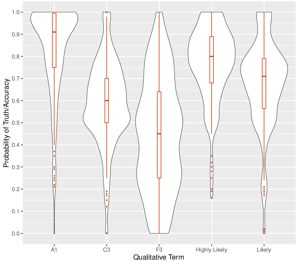
| Figure 5: Violin plots of probability equivalents
(Pe) of qualitative uncertainty terms.
An A1 is informant one that is deemed “completely reliable” and makes a
claim that is “completely credible”. A C3 informant is one that is deemed
“fairly reliable”, and makes a claim that is judged “possibly true”. A F3
informant is rated as “reliability cannot be judged”, and makes a claim denoted as “possibly true”. |
Figure 5 shows additional distributional information in violin plots.
Visually, among the source reliability/information credibility indicators,
PA1 has the tightest distribution, with
the median probability above .90, whereas
PF3 had the largest deviance among
participants. In terms of the two linguistic probabilities, as one might
expect, highly likely had less deviance among participants than
likely. This is consistent with use of these terms in some
lexicons wherein very likely represents a subset of
likely (e.g., Mastrandrea, Mach, Plattner & Matschoss, 2011) and
in studies that have compared the variability of interpretations of these
terms (e.g., Ho et al., 2015; Wintle, Fraser, Willis, Nicholson & Fidler,
2019). Table 5 shows mean values for each with 95% confidence intervals,
which confirms, on average, the inequality in equation (2), and provides
justification for our ordering of total evidential support in equation
(10).
Assuming se = Pe
(e.g., equations (6)–(8)), Table 6 displays the mean values of total
evidential support for each pair, again with similar ordering as equation
(10). In subsequent analyses, we re-order the pairs according to total
evidential support with Pairs 3, 1, and 2 representing low, medium and high
total evidential support, respectively.
| Table 5: Mean probability equivalents
(Pe) of qualitative uncertainty
terms.. M is the mean value whereas LB and
UB are 95% confidence interval lower and upper bounds. An A1
informant is one that is deemed “completely reliable” and makes a claim
that is “completely credible”. A C3 informant is one that is deemed
“fairly reliable”, and makes a claim that is judged “possibly true”. A
F3 informant is rated as “reliability cannot be judged”, and makes a claim denoted as “possibly true”. |
| P e | M | LB | UB |
| PHL | .77 | .75 | .79 |
| PL | .68 | .65 | .70 |
| PA1 | .83 | .81 | .86 |
| PC3 | .59 | .57 | .62 |
| PF3 | .44 | .41 | .47 |
| Table 6: Mean total evidential support by pair. M is the mean
value whereas LB and UB are 95% confidence interval
lower and upper bounds. |
| Pair | Level | M | LB | UB |
| 1 | Medium | 1.95 | 1.92 | 1.98 |
| 2 | High | 2.19 | 2.16 | 2.23 |
| 3 | Low | 1.80 | 1.76 | 1.84 |
3.2 Coherence of binary choice
As a first coherence test, we investigated the proportion of participants’
consistent responses between judgment and binary choice measures. Each
participant had a proportion score that ranged from 0 (0/6 matches) to 1
(6/6 matches). A response was marked as consistent if the choice
corresponded to the hypothesis to which a higher probability was assigned.
If EPi,j(GM)
= EPi,j(SA), either
choice was deemed to be consistent. This was viewed as the easiest form of
coherence, since the binary choice was made immediately after providing
probability judgments for the two hypotheses. If ACH improves the quality
of reasoning, then we might expect greater consistency between probability
judgment and choice in the ACH condition than in the control group.
However, we found no significant effect of method on the mean match rates
using either a parametric analysis (t[218] = 1.14,
p = .25, d = 0.15) or Fisher’s Exact Test, p =
.79. The overall match rate across all participants had a mean of .74 with
a 95% confidence interval of [.70, .77] (hereafter square brackets are
used to signify 95% confidence intervals).
3.3 Reliability
On the one hand, if ACH improves the consistency of reasoning due to its algorithmic steps, we might expect greater reliability of hypothesis
probabilities in the ACH condition than in the control group across
isomorphic cases. On the other hand, if the ACH inputs introduce noise
into the assessment process, we might expect less reliability in the ACH
condition than in the control condition across isomorphic cases. While we
did not expect total evidential support to influence reliability, we
tested the effect of method and total evidential support levels (low,
medium, and high) on reliability as measured by mean absolute deviation
(MAD) in equation (1) using a two-way mixed ANOVA. The results
are shown in Table 7. Indicating an overall significant level of
unreliability, the intercept was significant. The main effect of total
evidential support and its interaction with method were not significant.
However, the main effect of method approached significance (p =
.051). Unreliability was greater in the ACH condition (MAD = .22
[.19, .24]) than in the control condition (MAD = .18 [.16, .20]),
with Cohen’s d = 0.20 indicating a small effect size.
| Table 7: ANOVA results for mean absolute deviation (MAD)
measuring reliability between isomorphic case pairs. Total evidential
support consists of the three levels of support (high, medium, low). |
Factor | F | p |
Intercept | 226.59 | < .001 |
Method | 3.86 | .05 |
Total evidential support | 0.42 | .66 |
Method × Total evidential support | 0.52 | .60 |
3.4 Bias from complementarity
With bias from complementarity described in equation (11), negative values
indicate superadditivity, positive values indicate subadditivity and zero
indicates additivity, we expected bias from complementarity to generally
increase with total evidential support. If the results are consistent with
other studies featuring more than two hypotheses (Karvetski et al., 2020;
Mandel et al., 2018), where the control group featured subadditivity, we
would expect ACH to lead to larger degrees of subadditivity. We tested the
effect of method and total evidential support on bias from complementarity
(i.e., Δi,j) using a two-way mixed
ANOVA. Each of the three levels of total evidential support (low, medium,
and high) had two measures corresponding to the two cases comprising the
relevant level. The results are shown in Table 8. The intercept term
implies subadditivity was observed in all cases. The effect of method was
not significant, nor did method significantly interact with total
evidential support. However, the main effect of total evidential support
was significant. These results are consistent with an enhancement effect
leading to subadditivity, which was not mitigated nor exacerbated by ACH.
Collapsing across method and further investigating within the three
discrete levels of total evidential support, Fisher’s Least Significant
Difference tests showed that mean bias from complementarity was
significantly lower (at the α = .01 level) in the low pairs
(M = .13 [.10, .17]) than in the medium pairs (M = .18
[.14, .22]) or high pairs (M = .21 [.18, .25]), whereas the
difference between medium and high pairs was marginally significant
(p = .06).
Finally, granted the continuous definition of total evidential support as
defined in equations (6)–(8), we find the overall correlation between
bias from complementarity and total evidential support as r(225)
= .29, a medium effect. Using a more granular analysis, we also find
evidence of the enhancement effect within the discrete pairs. The
correlations between bias from complementarity and total evidential
support (as measured by equations (6)–(8)) within the three pairs (from
low to high) are as follows: r(225) = .39 [.26, .49], .31 [.18,
.44], and .29 [.15, .42],
| Table 8: ANOVA results for bias from complementarity. Total evidential
support consists of the three levels of support (high, medium, low). |
Factor | F | p |
Intercept | 65.97 | <.001 |
Method | 1.52 | .22 |
Total evidential support | 5.04 | <.001 |
Method × Total evidential support | 1.99 | .10 |
3.5 Bayesian coherence
As a third form of judgment coherence, we investigated the multiple degrees
to which participants’ elicited probabilities corresponded with the
corresponding Bayesian posterior probabilities. ACH is not a normative
model and exact correspondence with a Bayesian model is not expected.
Nevertheless, ACH is promoted as a method of improving analysts’ evidential evaluation and updating. Therefore, ACH might be expected to yield judgments that correspond more closely with a Bayesian
model than the unstructured judgments of participants in the control
group. The results in this subsection address that comparison.
For 10.1% of the sample, the elicited probabilities to the questions in
Table 1 resulted in at least one set of Bayesian posterior probabilities
that was undefined since there was a zero in the denominator of the
equation for Bayes’ theorem. In order to ensure the
Bayesian posterior values were properly defined for each participant, and
to respect Cromwell’s rule stating that prior
probabilities of 0 and 1 should be avoided unless these values can be
logically assumed (Lindley, 1991), for each participant we set elicited
uncertainty equivalents of 1 to .9999, and elicited uncertainty
equivalents of 0 to .0001 in order to ensure Bayesian posterior probabilities were calculable. This resulted in 31.7% of participants
having at least one elicited uncertainty equivalent set accordingly.
As an initial test of the effect of method on Bayesian coherence, we
calculated φ as the proportion of times the participants’ elicited
probabilities agreed with the Bayesian posterior values in terms of the
most likely hypothesis (with φ ranging from 0/6 to 6/6). Within
this calculation, the case where
EPi,j(GM) =
EPi,j(SA) was
considered agreement. As shown in Table 9, we did not find a significant
effect across methods for proportion of agreement.
We also calculated the mean absolute deviation (MAD) between the
Bayesian posterior probabilities and the elicited probabilities (both raw
and normalized), and averaged the mean absolute deviations across the six
cases for each participant. As Table 9 again shows, there was no
significant effect of method for either test. That is, participants were
no more or less coherent in the ACH condition than they were in the
control condition.
| Table 9: Comparisons of the elicited probabilities (both raw and
normalized) with Bayesian posterior probabilities in terms of agreement
percentage (φ) and mean absolute deviation
(MAD). M is the mean value whereas LB and
UB are 95% confidence interval lower and upper bounds. |
Measure | M | LB | UB | t | P | d |
φ | .65 | .62 | .67 | 0.46 | .65 | 0.06 |
MAD (raw elicited) | .31 | .30 | .32 | 1.01 | .31 | 0.13 |
MAD (normalized elicited) | .33 | .31 | .34 | 0.86 | .39 | 0.11 |
The averaged respective probabilities across methods are shown in Table 10,
and we see that the means values of the Bayesian posterior values and the
elicited normalized values agree in terms of the most likely hypothesis in
all cases (note that the elicited normalized values in Case 3 support both
hypotheses equally). However, demonstrating conservatism, the elicited
normalized probabilities are also closer to 50/50 than the corresponding
Bayesian estimates in all cases. Moreover, after removing bias from
complementarity by normalizing participants’ posterior probability
estimates, participants still do not update sufficiently to match the
Bayesian posterior probabilities derived from their equivalence ratings.
As an initial test of conservatism, we calculated the mean absolute
deviation (MAD) between the Bayesian probabilities and normalized
elicited probabilities with 50/50, and then averaged each mean absolute
deviation within participants. Using a paired t-test, the
average of the Bayesian MAD with 50/50 (M = .33 [.31,
.35]) was significantly greater than that of the normalized elicited
MAD (M = .13 [.11, .14]), t(226) = 23.20,
p < .001, d = 1.54. The effect size measure
shows that the degree of conservatism exhibited in this experiment was
very large.
| Table 10: Average Bayesian, elicited and normalized elicited probability
judgments by case. Hyp. = hypothesis, M is the mean value, and LB and
UB are 95% confidence interval lower and upper bounds. |
| | | Bayesian
(BP) | Elicited
(EP) | Normalized elicited (NEP) |
|
Case | Hyp. | M | LB | UB | M | LB | UB | M | | LB | UB |
| 1 | GM | .71 | .67 | .75 | .67 | .64 | .70 | .58 | | .56 | .60 |
| 1 | SA | .29 | .25 | .34 | .51 | .47 | .54 | .42 | | .40 | .44 |
| 2 | GM | .29 | .25 | .34 | .52 | .48 | .55 | .43 | | .41 | .46 |
| 2 | SA | .71 | .67 | .75 | .67 | .63 | .70 | .57 | | .55 | .59 |
| 3 | GM | .41 | .37 | .45 | .59 | .56 | .63 | .50 | | .48 | .53 |
| 3 | SA | .59 | .55 | .63 | .60 | .56 | .63 | .50 | | .47 | .52 |
| 4 | GM | .59 | .55 | .63 | .65 | .62 | .68 | .53 | | .51 | .56 |
| 4 | SA | .41 | .37 | .45 | .59 | .55 | .62 | .47 | | .44 | .49 |
| 5 | GM | .68 | .64 | .72 | .59 | .56 | .62 | .52 | | .49 | .54 |
| 5 | SA | .32 | .28 | .36 | .56 | .52 | .59 | .48 | | .46 | .51 |
| 6 | GM | .32 | .28 | .36 | .53 | .50 | .56 | .46 | | .44 | .49 |
| 6 | SA | .68 | .64 | .72 | .59 | .56 | .62 | .54 | | .52 | .56 |
3.6 Coherence of ACH ratings
Focusing only on participants in the ACH condition, we examined whether
consistency ratings of non-diagnostic evidence had a nil impact on
posterior probability judgments, as is normatively required. For example,
if one item of case evidence is that an F3 informant whose
“reliability cannot be judged” makes a claim denoted as “possibly true” that the suspect is a street artist, and the participant has
assessed PF3 = .5, then one should
assume the complementary claim (the suspect is a gang member) should have
the same probability of being true (i.e., .5). In the ACH matrix,
therefore, the two hypotheses within the row should each receive the same
consistency rating, and if a stricter constraint is applied, these values
should correspond to a neutral rating. Accordingly, the evidence
would have no impact on influencing the overall probability of the
hypotheses.
To examine this, for each item of evidence across the six cases, we
computed a differential consistency score,
δC, by comparing the inconsistencies
scores within each row of the ACH matrix. Consider the completed ACH
matrix in Figure 4, with the first item of evidence claiming it as
likely the suspect is a street artist, which is the hypothesis
favored by the evidence. Allowing
CF to refer to the consistency score
assigned to the hypothesis favored by the evidence (e.g.,
CF = 0 in Figure 4) and letting
CA refer to the consistency score
assigned to the alternative hypothesis (e.g.,
CA = -2), we can define our differential consistency score as δC =
CF −
CA (e.g.,
δC = 2, the net impact on the
hypothesis favored by the evidence).
In order to test the effect of a non-diagnostic rating, we scaled each
Pe around .5 as
|
Pe,SCALED = (Pe − .5) × 2.
(19) |
Such scaling implies non-diagnostic ratings (i.e.,
Pe = .5) are centered at 0, and
perfectly diagnostic ratings for a focal hypothesis (i.e.,
Pe = 1) are set to 1.
Using linear mixed regression analysis, we regressed
δC on the full set of scaled
uncertainty terms across all participants, and found the intercept was
significant, B = 0.233, SE = 0.074, Wald = 9.92,
p = .002, as was the slope term, B = 0.502, SE
= 0.082, Wald = 37.48, p < .001; model
R2 = .055. Given the scaling, the
positive intercept shows that evidence linked to non-diagnostic
ratings had a positive mean impact on ACH consistency scores, whereas
perfectly diagnostic ratings for a hypothesis favoured by the evidence
corresponds to a mean δC =
0.735 (0.502 + 0.233). This implies that the impact of evidence associated
with non-diagnostic ratings is roughly 32% of the impact of evidence
associated with perfectly diagnostic ratings.
To rule out the possibility that participants may have treated consistent
information as representing positive values rather than zero (which again
is the typical ACH convention, and the one used within the experiment), we
replaced the consistency scores used in the preceding analyses with scores
that assigned positive values to consistent evidence (e.g., C = 1 and CC =
2 rather than either equaling 0) and repeated the regression analysis.
Once again, we found significant effects for the intercept, B =
0.522, SE = 0.152, Wald = 11.34, p = .001, and the
slope term, B = 1.20, SE = 0.165, Wald = 52.89,
p < .001, with R2 =
0.072. As in the preceding analysis, there is a mean positive impact for
evidence associated with a non-diagnostic ratings corresponding to roughly
30% of the impact of evidence associated with a perfectly
diagnostic rating for a favored hypothesis.
4 Discussion
The present research sheds additional light on the effectiveness of ACH,
one of the intelligence community’s most highly promoted structured
analytic techniques for helping intelligence analysts sift through
uncertain evidence in order to assess the relative likelihood of competing
hypotheses. Consistent with recent research (Dhami et al., 2019; Karvetski
et al., 2020; Mandel et al., 2018; Whitesmith, 2019), we found no benefit
conferred by ACH when compared to a no-SAT control. Participants who used
ACH prior to judging posterior probabilities from uncertain evidence were
no more additive, coherent in a Bayesian sense, consistent with their
binary choices, or able to avoid conservatism than participants who did
not use the technique. Participants who used ACH were less reliable across
isomorphic cases than control participants who were not asked to use any
particular technique, although the effect was small. Moreover,
participants who used ACH showed evidence of pseudo-diagnostic evaluation
of evidential support for competing hypotheses.
These findings add to the previous literature on the evaluation of ACH in
improving facets of judgment quality in at least two respects. First, the
range of coherence-related measures of judgment quality that were examined
was extended. To the best of our knowledge, intra-individual reliability
of judgments, conservatism in belief updating, and consistency with binary
choice have not been previously investigated in relation to ACH. Second,
the present research used a task that involved reasoning from
qualitatively described, uncertain evidence, which, compared to other
recent studies (e.g., Karvetski et al., 2020; Mandel et al., 2018) better
approximates conditions in which intelligence analysts and criminal
investigators encounter evidence. That is, unlike the aforementioned
studies, the present research used verbal probabilities to convey
likelihood, which—for better or worse—is the communication method
currently favored by most intelligence organizations (Dhami & Mandel,
2020; Mandel & Irwin, 2020). As well, the prior studies asked subjects to assume that information presented was perfectly accurate,
whereas in the present research, uncertainty about source reliability and
information credibility was conveyed as it often is in raw human
intelligence reports (Irwin & Mandel, 2019; Samet, 1975). Therefore, the
present research not only coheres with the findings of recent studies of
ACH, it also improves the external validity of the body of evidence
bearing on the method.
The finding that ACH did not improve reliability (and in fact lowers
reliability slightly) contradicts the widely held, but largely untested,
assumption in intelligence communities that structured analytic methods
will be more reliable than an ad hoc “intuitive” analytic judgments (Chang
et al., 2018; Mandel, 2020). A potential reason ACH might decrease
reliability is that the technique may make the judgment process more
cumbersome or susceptible to various degrees of interpretation. For
instance, as noted earlier, fundamental concepts such as the meaning of
“consistency” are left undefined in documentation describing ACH (Heuer &
Pherson, 2014). Chang et al. (2018) used the term noise neglect
to refer to the intelligence community’s failure to attend to this
potential downside of SATs. SATs like ACH also shift the analyst’s
attention from the substantive topic of analysis to the implementation of
the technique’s many steps. Refocusing on the proper implementation of a
purportedly judgment-enhancing technique could, in principle, steer
attention away from deliberative reasoning directed towards the
substantive reasoning challenges that would motivate the use of such
techniques in the first place. The cost of misdirected attention is, of
course, a function of the analysts’ potential for sound reasoning. An
implication of this perspective is that ACH may incur the greatest costs
among the best analysts while perhaps offering some ameliorative benefit
to the worst performers. This hypothesis could be tested in future
research.
In our experiment, we observed a clear violation of the complementarity
axiom across the two hypotheses. Although ACH did not exacerbate this bias
as in previous studies (Mandel et al., 2018; Karvetski et al., 2020), it
did not mitigate the bias either. Also, since adherence to the
complementarity axiom for binary complements is axiomatic in support
theory (Rottenstreich & Tversky, 1997; Tversky & Koehler, 1994), the
present findings contradict the theory in that regard. Rather, our data
support the hypothesis that additivity violations with binary complements
are predictable on the basis of total evidential support summed across
hypotheses and sources. This particular finding is comparable with the
general findings of Idson et al. (2001) and Villejoubert and Mandel
(2002). Whereas we observed subadditivity exclusively in our study, and
Idson et al. (2001) and Villejoubert and Mandel (2002) observed a
combination of subadditivity and superadditivity, the present findings, in
fact, are consistent with those studies. This is because all cases in the
present experiment had total evidential support exceeding unity, whereas
total support was manipulated to be either high or low in the
aforementioned studies. Although our finding of subadditivity is
inconsistent with the formal binary complementarity axiom of support
theory, the notion that subadditivity will increase with support is in
fact central to support theory and referred to as the enhancement
effect (Koehler, Brenner, & Tversky, 1997).
In the present research, we were able to compare two sets of posterior
probabilities, those explicitly elicited from participants in response to
the specific case materials and those derived from their initial
probability estimates in which they provided numeric probability
equivalents for the terms they would subsequently encounter in the cases.
Using these substitutes in conjunction with Bayes’ theorem, we measured
the extent to which the implicit (Bayesian) and explicit estimates
differed in absolute terms. There was substantial difference that was
unaffected by whether or not ACH was used, and this difference persisted
even when deviations due to complementarity violations were subtracted.
There are multiple reasons for such disagreement. One possibility is that
the initial estimates are unreliable and that even moments later, the
quantitative equivalencies were inaccessible and new estimates constructed
on the fly or “online” were produced that varied with the original values
(e.g., see Hastie & Park, 1986). A second possibility is that the initial
estimates were adjusted in light of the context in which they appeared in
some systematic manner. Brun and Teigen (1988) found that, depending on
the study they examined, participants either assigned higher or lower
numeric probability equivalents to verbal probabilities when they were
presented in context compared to when they were presented out of context.
In future research, one could elicit in-context numeric equivalents either
instead of the pre-case estimates taken in the present experiment or else
in addition to them. Of course, another possibility is that the deviations
result from a failure to correctly integrate the evidence, which would be
robust in other designs and which is simply not improved by use of ACH.
The findings also showed that within the ACH condition, evidence that
corresponded to a non-diagnostic truth/accuracy rating still had a
positive contribution or impact towards the hypothesis favored at face
value by the evidence. Not only was the net impact of non-diagnostic
evidence significantly differing from zero, it had about 30% of the
impact of evidence with a truth/accuracy rating that was completely
diagnostic for a focal hypothesis. This is potentially detrimental for it
indicates that ACH users reasoning about a case with one diagnostic A1
informant claiming Hypothesis 1 and three potentially non-diagnostic F3
informants claiming Hypothesis 2 may judge the alternatives to be
equiprobable. We cannot rule out that a similar bias might have been
present in the control condition because we did not measure ratings of
evidential consistency with the alternative hypotheses. However, future
research could, for example, elicit such ratings after posterior
probability judgments were made, and could also expand the variety of evidential inputs used within the format of the exercise. For instance,
future studies could systematically vary source reliability levels
independently of information credibility levels to understand if one is
deemed more influential in weighing evidence.
Overall, our findings highlight the importance of directly testing the
effectiveness of methods used in practice to improve judgment and
decision-making, and these findings underscore the appropriateness of
recent calls for better methodological evaluation in intelligence
communities (Chang et al., 2018; Dhami et al., 2015; Mandel, 2020; Mandel
& Tetlock, 2018). The method we tested in this research—ACH—is not merely
one of dozens of methods advocated for use by several allied intelligence
communities, it is one of most widely taught and promoted methods. Given
the resources spent to train and encourage analysts to use ACH, one might
expect to see some positive effects on judgment. In this research and in
other recent studies (e.g., Dhami et al., 2019; Karvetski et al., 2020;
Mandel et al., 2018; Whitesmith, 2019), however, ACH had either no benefit
on measures of judgment quality or produced a decrease in performance.
Nevertheless, we do not wish to overstate our claims. Notwithstanding the
present experiment’s more realistic features, such as imprecise,
qualitative evidence including information about source reliability and
information credibility, which were presented using alphanumeric codes
commonly used in the defense and intelligence communities (Irwin &
Mandel, 2019; Samet, 1975), the experimental cases invariably featured
three items of evidence and two hypotheses. Future research might examine
tasks that include larger troves of evidence and perhaps more alternative
hypotheses, and with real analysts. Note, however, that the task used by
Mandel et al. (2018) included twelve probabilistic cues and four
hypotheses having variable prior probabilities. Real intelligence analysts
in that experiment nevertheless performed more poorly using ACH than their
counterparts who were left to their unaided reasoning. The mounting
evidence from multiple experiments with different samples, tasks, and
experimental designs in recent years indicates that ACH does not benefit
judgment and, in fact, might impair judgment. Although more research on the topic is warranted, intelligence communities that rely on ACH as a
structured analytic method to support intelligence analysis should also
take seriously the implications of the current body of evidence and
consider alternative methods for improving judgment quality.
References
Ayton, P. (1997). How to be incoherent and seductive: Bookmakers’ odds and
support theory. Organizational Behavior and Human Decision
Processes, 72, 99–115.
Barnes, A. (2016). Making intelligence analysis more intelligent: Using
numeric probabilities. Intelligence and National Security, 31,
327–344.
Brun, W., & Teigen, K. H. (1988). Verbal probabilities: Ambiguous,
context- dependent, or both? Organizational Behavior and Human
Decision Processes, 41, 390–404.
Chang, W., Berdini, E. ,, Mandel, D. R., & Tetlock, P. E. (2018).
Restructuring structured analytic techniques in intelligence.
Intelligence and National Security, 33, 337–356.
Dhami, M. K., Belton, I., & Mandel, D. R. (2019). The ‘Analysis of
Competing Hypotheses’ in intelligence analysis. Applied Cognitive
Psychology, 33, 1080–1090.
Dhami, M. K., & Mandel, D. R. (2013). How do defendants choose their trial
court? Evidence for a heuristic processing account. Judgment and
Decision Making, 8, 552–560.
Dhami, M. K., & Mandel, D. R. (2020). Words or numbers? Communicating
probability in intelligence analysis. American Psychologist.
Advance online publication. http://dx.doi.org/10.1037/amp0000637.
Dhami, M. K., Mandel, D. R., Mellers, B. A., & Tetlock, P. E. (2015).
Improving intelligence analysis with decision science.
Perspectives on Psychological Science, 10, 753–757.
Drogin, B., & Goetz, J. (2005). How U.S. Fell Under the Spell of
“Curveball”, Los Angeles Times, 20 Nov. 2005.
Edwards, W. (1968). Conservatism in human information processing. In B.
Kleinmuntz Ed.), Formal representation of human judgment (pp.
17–52). New York, NY: Wiley.
Fan, Y., Budescu, D. V., Mandel, D., & Himmelstein, M. (2019). Improving
accuracy by coherence weighting of direct and ratio probability
judgments. Decision Analysis, 16, 197–217.
Hammond, K. R. (2000). Coherence and correspondence theories in judgment
and decision making. In T. Connolly, H. R. Arkes, & K. R. Hammond
(Eds.), Judgment and decision making: An interdisciplinary
reader (pp. 53–65). Cambridge, MA: Cambridge University Press.
Hastie, R., & Park, B. (1986). The relationship between memory and
judgment depends on whether the judgment task is memory-based or on-line.
Psychological Review, 93, 258–368.
Heuer, R. J., & Center for the Study of Intelligence (US). (1999).
Psychology of intelligence analysis. Washington, DC: Center for
the Study of Intelligence, Central Intelligence Agency.
Heuer, R. J. (2005). How does Analysis of Competing Hypotheses
(ACH) improve intelligence analysis? Accessed February
19th, 2018 at:
http://www.pherson.org/wp-content/uploads/2013/06/06.-How-Does-ACH-Improve-Analysis\_FINAL.pdf.
Heuer, R. J., Jr., & Pherson, R. H. (2014). Structured analytic
techniques for intelligence analysis. Washington, DC: CQ Press.
Ho, E. Budescu, D. V., Dhami, M. K., & Mandel, D. R. (2015). Improving the
communication of uncertainty in climate science and intelligence analysis.
Behavioral Science & Policy, 1, 43–55.
Idson, L. C., Krantz, D. H., Osherson, D., & Bonini, N. (2001). The
relation between probability and evidence judgment: An extension of
support theory. Journal of Risk and Uncertainty, 22,
227–249.
Irwin, D. & Mandel, D. R. (2019). Improving information evaluation for
intelligence production. Intelligence and National Security,
34, 503–525.
Kahneman, D., & Tversky, A. (1972). Subjective probability: A judgment of
representativeness. Cognitive Psychology, 3, 430–454.
Karvetski, C. W., Olson, K. C., Gantz, D. T., & Cross, G. A. (2013). Structuring and analyzing competing hypotheses with Bayesian networks for
intelligence analysis. EURO Journal on Decision Processes, 1,
205–231.
Karvetski, C. W., Olson, K. C., Mandel, D. R., & Twardy, C. R. (2013).Probabilistic coherence weighting for optimizing expert forecasts.
Decision Analysis, 10, 305–326.
Karvetski, C.W., Mandel, D.R., & Irwin, I., (2020). Improving probability
judgment in intelligence analysis: From structured analysis to statistical
aggregation. Risk Analysis, 40, 10140-1057.
Koehler, D.J, L. A. Brenner, & Tversky, A. (1997). The enhancement effect
in probability judgment. Journal of Behavioral Decision Making,
10, 293–313.
Lehner, P. E., Adelman, L., Cheikes, B. A., & Brown, M. J. (2008).
Confirmation bias in complex analyses. IEEE Transactions on
Systems, Man, and Cybernetics - Part A: Systems and Humans, 38, 584–592.
Lindley, D. V. (1991). Making decisions (2nd
ed.). London, UK: John Wiley and Sons, Ltd.
Macchi, L., Osherson, D., & Krantz, D. H. (1999). A note on superadditive
probability judgment. Psychological Review, 106, 210–214.
Mandel, D. R. (2005). Are risk assessments of a terrorist attack
coherent? Journal of Experimental Psychology: Applied, 11,
277–288.
Mandel, D. R. (2008). Violations of coherence in subjective probability: A
representational and assessment processes account. Cognition,
106, 130–156.
Mandel, D.R. (2015a). Accuracy of intelligence forecasts from the
intelligence consumer’s perspective. Policy Insights from the
Behavioral and Brain Sciences, 2, 111–120.
Mandel, D. R. (2015b). Instruction in information structuring improves
Bayesian judgment in intelligence analysts. Frontiers in
Psychology, 6, 387, https://doi.org/10.3389/fpsyg.2015.00387.
Mandel, D. R. (2019). Too soon to tell if the US intelligence community
prediction market is more accurate than intelligence reports: Commentary
on Stastny and Lehner (2018). Judgment and Decision Making, 14,
288–292.
Mandel, D. R. (2020). The occasional maverick of analytic
tradecraft. Intelligence and National Security, 35, 438–443.
Mandel, D. R., & Irwin, D. (2020). Uncertainty, intelligence, and
national security decision-making. International Journal of
Intelligence and CounterIntelligence. https://doi.org/10.1080/08850607.2020.1809056.
Mandel, D. R., Karvetski, C. W., & Dhami, M. K. (2018). Boosting
intelligence analysts’ judgment accuracy: What works,
what fails? Judgment and Decision Making, 13, 607–621.
Mandel, D. R., & Dhami, M. K. (2018). Experiment on the
probabilistic interpretation of source reliability and information
credibility indicators in NATO intelligence doctrine. Unpublished data.
Mandel, D. R., & Tetlock, P. E. (2018). Correcting judgment correctives in
national security intelligence. Frontiers in Psychology, 9, 2640,
https://doi.org/10.3389/fpsyg.2018.02640.
Mastrandrea, M. D., Mach, K. J., Plattner, G., & Matschoss, P. R. (2011).
The IPCC AR5 guidance note on consistent treatment of uncertainties: A
common approach across the working groups. Climatic Change, 108,
675–691.
Mellers, B. A., Baker, J. D., Chen, E., Mandel, D. R., & Tetlock, P. E.
(2017). How generalizable is good judgment? A multi-task, multi-benchmark
study. Judgment and Decision Making, 12, 369–381.
Mosteller, F., & Youtz, C. (1990). Quantifying probabilistic expressions.
Statistical Science, 5, 2–12.
Nickerson, R. S. (1998). Confirmation bias: A ubiquitous phenomenon in many
guises. Review of General Psychology, 2, 175–220.
North Atlantic Treaty Organization (2015). Allied joint doctrine for intelligence procedures: AJP-2.1 (Edition B, Version 1). Brussels,
Belgium: author.
Office of the Director of National Intelligence (2015).
Intelligence community directive
203: Analytic standards. Washington, DC: author. Available from
http://fas.org/irp/dni/icd/icd-203.pdf.
Palo Alto Research Center (PARC). (2006). ACH: Version 2.0.3.
Available from
http://www2.parc.com/istl/projects/ach/ach.html.
Phillips, L. D., & Edwards, W. (1966). Conservatism in a simple
probability inference task. Journal of Experimental Psychology, 72, 346–354.
Rottenstreich, Y., & Tversky, A. (1997). Unpacking, repacking, and
anchoring: Advances in support theory. Psychological Review, 104,
406–415.
Samet, M. G. (1975). Quantitative interpretation of two qualitative scales
used to rate military intelligence. Human Factors, 17,
192–202.
Sedlmeier, P., & Gigerenzer, G. (2001). Teaching Bayesian reasoning in
less than two hours. Journal of Experimental Psychology: General,
130, 380–400.
Slowiaczek, L. M., Klayman, J., Sherman, S. J., & Skov, R. B. (1992).
Information selection and use in hypothesis testing: What is a good
question, and what is a good answer? Memory & Cognition, 20,
392–405.
Stastny, B. J., & Lehner, P. E. (2018). Comparative evaluation of the
forecast accuracy of analysis reports and a prediction market.
Judgment and Decision Making, 13, 202–211.
Tombu, M., & Mandel, D. R. (2015). When does framing influence
preferences, risk perceptions, and risk attitudes? The explicated valence
account. Journal of Behavioral Decision Making, 28, 464–476.
Tversky, A., & Fox, C. R. (1995). Weighing risk and uncertainty.
Psychological Review, 102, 269–283.
Tversky, A., & Koehler, D. J. (1994). Support theory: a nonextensional
representation of subjective probability. Psychological
Review, 101, 547–567.
US Government (2009). A tradecraft primer: Structured analytic
techniques for improving intelligence analysis. Washington, DC: Center
for the Study of Intelligence Analysis.
Villejoubert, G., & Mandel, D. R. (2002). The inverse fallacy: An account
of deviations from Bayes’s theorem and the additivity principle.
Memory and Cognition, 30, 171–178.
Wallsten, T. S., Budescu, D. V., & Zwick, R. (1993). Comparing the
calibration and coherence of numerical and verbal probability judgments.
Management Science, 39, 176–190.
Wang, G., Kulkarni, S. R., Poor, H. V. (2011). Aggregating large sets of
probabilistic forecasts by weighted coherent adjustment. Decision
Analysis, 8, 128–144.
Whitesmith, M. (2019). The efficacy of ACH in mitigating serial position
effects and confirmation bias in an intelligence analysis scenario.
Intelligence and National Security, 34, 225–242.
Wintle, B. C., Fraser, H., Willis, B. C., Nicholson, A. E., & Fidler, F.
(2019). Verbal probabilities: Very likely to be somewhat more confusing
than numbers. PLOS ONE, 14, e0213522. http://dx.doi.org/10.1371/journal.pone.0213522.
This document was translated from LATEX by
HEVEA.