Judgment and Decision Making, Vol. 16, No. 2, March 2021, pp. 323-362
Forecasting forecaster accuracy: Contributions of past performance and individual differences
Mark Himmelstein* #
Pavel Atanasov$
David V. Budescua
|
Abstract:
A growing body of research indicates that forecasting skill is a unique and stable trait: forecasters with a track record of high accuracy tend to maintain this record. But how does one identify skilled forecasters effectively? We address this question using data collected during two seasons of a longitudinal geopolitical forecasting tournament. Our first analysis, which compares psychometric traits assessed prior to forecasting, indicates intelligence consistently predicts accuracy. Next, using methods adapted from classical test theory and item response theory, we model latent forecasting skill based on the forecasters’ past accuracy, while accounting for the timing of their forecasts relative to question resolution. Our results suggest these methods perform better at assessing forecasting skill than simpler methods employed by many previous studies. By parsing the data at different time points during the competitions, we assess the relative importance of each information source over time. When past performance information is limited, psychometric traits are useful predictors of future performance, but, as more information becomes available, past performance becomes the stronger predictor of future accuracy. Finally, we demonstrate the predictive validity of these results on out-of-sample data, and their utility in producing performance weights for wisdom-of-crowds aggregations.
Keywords: forecasting, individual differences, item response models, longitudinal analysis, skill assessment, wisdom-of-crowds, hybrid forecasting competition
1 Introduction
From ancient oracles to modern prediction markets, humanity has long been fascinated by the prospect of predicting future events. While data-driven approaches to prediction have grown in popularity, human forecasting remains important, especially in data-sparse settings. Human forecasting is a unique psychological process. Unlike strictly intellective tasks, driven entirely by domain-specific knowledge, or judgmental tasks that relate to preferences, values and opinions, forecasting features a combination of intellective and judgmental processes (Fan et al., 2019; Stael von Holstein, 1970; Wallsten & Budescu, 1983). What makes a good forecaster? Is it someone who is highly knowledgeable regarding the particular subject being forecasted? Someone who excels at probabilistic reasoning and inference? Perhaps a combination of both? Or perhaps neither, and forecasting is a unique skill unto its own.
We address these questions by examining data collected during several geopolitical forecasting tournaments. Forecasting tournaments are a relatively recent innovation in which participants make repeated forecasts for numerous events over a specified period of time, and the winners are determined by objective scoring rules that reflect the forecasts’ accuracy (Tetlock et al., 2014). These tournaments provide an information-rich research environment for studying processes related to human forecasting, including the correlates of forecasting skill.
1.1 Forecasting Tournaments
In 2011, the Intelligence Advanced Research Projects Activity (IARPA) launched the Aggregative Contingent Estimation (ACE) program (Tetlock et al., 2014). The goal of the ACE program was to develop highly accurate forecasting systems by invoking wisdom-of-crowds (WoC) principles (Budescu & Chen, 2014; Davis-Stober et al., 2014; Surowiecki, 2005). The WoC predicts that crowdsourced aggregations of judgments of many forecasters will substantially outperform individual forecasters, including highly trained experts. To incentivize participation, ACE was structured as a series of forecasting competitions in which participants forecasted the same events and were assessed by predetermined criteria.
Multiple research groups were recruited and tasked with developing forecasting systems. Each group developed their own platform and hosted a separate forecasting tournament based on an identical set of questions, which covered several domains with forecasting horizons ranging from a few weeks to several months. One such research group was the Good Judgment Project (GJP, Mellers et al., 2014). A key feature of the GJP approach was identifying highly skilled individual forecasters, or Superforecasters (Mellers, et al., 2015b; Tetlock & Gardner, 2016). By identifying these individuals, GJP was able to both cultivate their performance and develop weighted aggregation methods that relied more heavily on their judgments without sacrificing the benefits of the WoC approach (Atanasov et al., 2017; Budescu & Chen, 2014; Chen et al., 2016; Karvetski et al., 2013).
In 2017, IARPA launched a follow-up tournament: the Hybrid Forecasting Competition (HFC) (IARPA, 2018). HFC was a competition between three research groups, whose goal was to find effective methods for combining human judgment with machine models in forecasting. HFC was divided into two seasons, structured as Randomized Controlled Trials (RCTs)1 with forecasters randomly assigned to research groups at the start of each season. Each season lasted six to eight months. The authors were members of the Synergistic Anticipation of Geopolitical Events (SAGE) research group (Morstatter et al., 2019).
This RCT structure raised a new challenge to the crowd prediction approach. As researchers had only a limited time window to identify skilled forecasters, it was critical to do so as early as possible and develop optimal weighting schemes based on the information available at any given moment. Although the constraints of the RCT structure did not allow research groups to gain an edge by recruiting superior forecasters, they provided a more controlled research environment. As such, these tournaments provide an ideal opportunity to generalize and extend past results regarding individual forecasting performance.
What constitutes a skilled forecaster? Are there certain traits that reliably identify skilled forecasters? If so, how can we leverage and balance these traits in the presence or absence of information on past forecasting performance? Our goal is to address these questions and understand the best ways to measure and identify forecasting skill by using data collected by the SAGE research group during the two seasons of the HFC program.
1.2 Individual Forecaster Assessment
A critical result from the GJP research was that forecasting skill is a relatively stable trait (Mellers, et al., 2015a; Mellers, et al., 2015b; Tetlock & Gardner, 2016). Forecasters who have performed well in the past, and forecasters who are more active and engaged, are more likely than others to produce accurate forecasts. In other words, it is possible to reliably predict future accuracy from past performance and task engagement (e.g., Chen et al. 2016; Mellers, et al., 2015b). Psychometric theory provides methods for measuring trait levels across individuals.
Before describing these psychometric methods, it is important to define our
usage of certain terms. Accuracy is a property of an actual
forecast — namely, how well it represented the eventual
outcome. Ability or skill is a latent trait that drives
the degree to which forecasters predictably vary in accuracy. Finally,
performance is a general term representing a forecaster’s
empirical contributions during a forecasting competition. This term refers
primarily to empirical estimates of ability, but it can also include the
extent of active participation.
The distinction between performance and skill is subtle, but important. Performance is a function of an individual’s behavior as well as the task. If an athlete is playing one-on-one basketball and scores a basket, she is awarded two points. The total score at the end of a game is a measure of player performance, which can be compared with an opponent’s performance to determine a winner. If these two players were to play again, it is highly unlikely the game would end with the exact same score; and if a players’ opponent changed, it is even less likely the score would be repeated. As this example suggests, performance is local, specific and unreliable — it varies from elicitation to elicitation — as other contextual and/or stochastic factors influence the result as well. Skill, on the other hand, is a global and stable latent ability, or trait, intrinsic to an individual. Traits are not directly observable, but they are thought to predict behavior, and thus performance. Performance can be considered an unbiased estimator of skill, but only when certain assumptions are met.
1.3 Psychometric Theory
In classical test theory (CTT), observed performance is considered a combination of an individual’s “true” level on a given trait, and residual error (Bandalos, 2018; Lord & Novick, 1968; Novick, 1966). The canonical CCT model, where X refers to an observed score, T an individual’s unobservable true trait level, and E to residual error, is given as:
This equation is mirrored in the literature on forecasting, which partitions measures of average individual accuracy into skill components perturbed by residual error (Mandel & Barnes, 2014; Murphy, 1973; Wallsten & Budescu, 1983). If residual error is assumed to be random with a mean of 0, an observed score is an unbiased estimate of the trait level, as measured on the scale of the performance metric. Several, often unrealistic conditions are required for this assumption to hold. For example, all forecasters must either forecast the same questions, or variation in question difficulties must be accounted for. In the context of longitudinal forecasting, the timing of a forecast also plays a role: how does the timing of forecasts about the same event influence difficulty? Addressing these issues is critical for applying the classical psychometric model to a forecasting tournament in which participants self-select when and which events to forecast.
An alternative psychometric approach, designed in part to address these issues, is known as Item Response Theory (IRT) (Embretson & Reise, 2013; Lord & Novick, 1968). Whereas in CTT, items are typically treated as equivalent components of a total score, IRT is based on the principle that different items carry unique information about the trait they are supposed to measure. Originally developed for measuring trait levels based on educational tests, the most well-known IRT models estimate the conditional probability that an individual provides a certain response to each item, given their level on the relevant trait as well as parameters that define each item’s diagnostic properties.2 One of the most common IRT models is the two-parameter logistic model. The two parameters refer to each item’s two diagnostic parameters: difficulty (b) and discrimination (a). The trait level of participants is represented by a person-specific parameter, θ. Where Xij is a binary response variable for person j on item i, this model is:
In this model, bi represents the location on the latent trait scale such that, for item i, a person with θj=bi will answer the item correctly with probability = .5, while ai represents a steepness parameter which determines how well item i discriminates values of θ near bi. The scale for θ is computationally indeterminate. Conventionally it is scaled such that θ ∼ N(0,1), and the scale for b is determined by the scale for θ. In this model, each item can be considered to have its own unique function, known as an item response function.
Applied to forecasting, one can think of the standard classical test theory model as producing a direct measure of skill, representing the mean accuracy of all forecasts a forecaster makes, where all forecasts are assigned equal weight, regardless of the timing or event being forecasted. One can, likewise, think of measures based on IRT as a weighted average of a forecasters’ accuracy across all of their forecasts, where the weights are a function of the event (or item) specific parameters (see Bo et al., 2017). As such the IRT measures should be more sensitive to the specific events people choose to forecast.
1.4 Longitudinal Forecasting
A unique problem in a longitudinal forecasting setting is the effect of time. Since all forecasting questions have a pre-determined resolution time, forecasting gets easier as time passes. In some cases, this reflects the structure of the forecasting problem, as options are restricted or ruled out, similar to how the number of baseball teams that can theoretically win the World Series is reduced as other teams are eliminated during earlier playoff rounds. In other cases, this simply reflects the accumulation of information over time, such as a sudden shortage of a given commodity increasing its price. Figure 1 demonstrates changes in average accuracy over time across all HFC questions that were at least 12 weeks in duration and demonstrates how empirical accuracy improved monotonically as a function of time to resolution.
Accounting for timing represents a non-trivial problem in assessing a forecaster’s skill. Merkle et al. (2016) used an IRT-based approach to adjust for the effect of time on accuracy, however they did not explicitly link their results to proper scoring rules. Bo et al. (2017) demonstrated that IRT methods can be linked to proper scoring rules, however they did not consider changes in accuracy over time. We demonstrate that it is possible to combine these methods and link an IRT-based approach to proper scoring rules while accounting for temporal changes in forecasting difficulty. We also demonstrate a novel approach to direct accuracy assessment that can account for temporal changes in difficulty, which bears more resemblance to CTT methods.
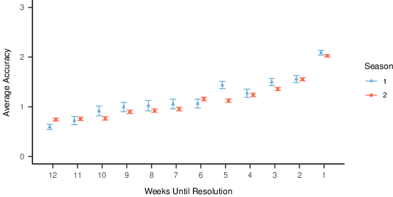
| Figure 1: Average accuracy of forecasts as a function of time for all questions of at least 12 weeks in duration. Average accuracy refers to normalized accuracy scores (see methods). For a binary forecasting question, normalized accuracy of 0 represents a probability of exactly .5 assigned to the correct option. Higher values represent more accurate forecasts. |
In addition to expanding on previous studies that have applied IRT models to probability judgments (Bo et al., 2017; Merkle et al., 2016), we also intend to demonstrate their practical applications. Both previous studies relied on the same dataset generated by GJP. These data were based on a subset of questions with especially high response rates, which were selected to avoid potential complications related to data sparsity. However, as Merkle et al. (2017) point out, question selection is an important and frequently neglected dimension of performance. Focusing only on the most popular questions potentially limits the generalizability of these foundational results. We apply IRT models across all forecasting questions included in HFC, and demonstrate their practical applications even when less popular questions are included.
1.5 The Cold Start Problem
One inherent problem when using past performance to identify high ability forecasters is that this information is not immediately available. Without performance information available to estimate skill, these approaches are of no use. This is an example of the cold start problem, which is a common issue in systems which use past behavior to predict future behavior (Lika et al., 2014; Schein et al., 2002).
Fortunately, results generated by the GJP indicate that forecasting ability can be modeled using other trait measures that are accessible even in the absence of past performance information. Mellers, et al. (2015a) found that general intelligence — particularly quantitative reasoning ability (Cokely et al., 2012) and reflective thinking (Baron et al., 2015; Frederick, 2005) — along with open mindedness (Stanovich & West, 1997) and relevant subject knowledge were particularly helpful in predicting forecasting skill. Moreover, skilled forecasters tended to be highly coherent, i.e., their judgments followed the axioms of propositional logic, and well calibrated, i.e., they assigned probabilities to events which correspond, on average, with the actual outcomes (Karvetski et al., 2013; Mellers et al., 2017; Moore et al., 2016). Coherence and calibration have been found to be important factors in other tasks related to probability judgment as well (Fan et al., 2019). Other approaches to early skill identification have focused on proxy measures for accuracy available before forecasting questions resolve (Witkowski, et al., 2017), or on behaviors observable in real-time, such as forecast updating (Atanasov et al., 2020).
Cooke’s method (also known as the “classical model”) in which one administers a series of domain specific general knowledge calibration questions provides an alternative solution to the cold start problem. The participants provide responses and rate their degree of confidence in those responses, prior to eliciting any actual forecasts (Aspinall, 2010; Colson & Cooke, 2018; Hanea et al., 2018). While domain knowledge can be a helpful predictor of forecasting accuracy (Mellers, et al., 2015a), these confidence ratings also provide a measure of calibration by comparing a forecaster’s confidence to actual performance on these domain questions. Calibration is an important component of any probability judgment, and people tend to be overconfident in their judgments about their performance to both general knowledge questionnaires (Brenner et al., 1996) and forecasts (Moore et al., 2016).
1.6 Research Questions and Hypotheses
Our goal is to determine how to best identify high performing forecasters and to demonstrate how different sources of information can be utilized to achieve this goal. We seek to demonstrate how helpful individual difference measures are by themselves when no past performance information is available, and how much benefit is added over time as performance information becomes available. Past studies have shown both sources of information can identify forecasting skill, but no study has shown how they complement each other, or how the relative importance of the sources changes as performance data accumulate. To answer this question, we first generalize past findings that have demonstrated the utility of performance and individual difference information separately, before examining their joint contributions at various time points. We further synthesize the IRT approaches of Merkle et al. (2016) and Bo et al. (2017) to link our model’s performance-based estimates of forecasting ability to proper scoring rules, while accounting for changes in difficulty for forecasting different events over time, as well as propose a new time-sensitive approach to direct assessment. The first three hypotheses pertain to generalization of prior research, while the last three are new.
Hypothesis 1. Individual difference measures of intelligence, cognitive style, domain knowledge and overconfidence in domain knowledge (calibration) will predict accuracy of future forecasts. (Generalization)
Hypothesis 2. Empirical measures of forecaster ability based on the accuracy of their forecasts will be stable over time. (Generalization)
Hypothesis 3. IRT-based estimates of forecasting skill (based on past performance) will predict accuracy of future forecasts better than direct skill measures. (Generalization)
Hypothesis 4. Adjusting for forecast timing relative to event resolution will improve direct ability assessment methods. (New hypothesis)
Hypothesis 5. As information about performance becomes available, these performance-based skill estimates will surpass individual difference measures assessed in advance at predicting accuracy of future forecasts. (New hypothesis)
Hypothesis 6. Performance weights using a combination of individual difference information and IRT-based skill assessment will optimize wisdom-of-crowds aggregation relative to weights that combine direct skill assessment measures and individual differences. However, weights that combine direct skill assessment measures and individual differences will still perform better than weights that rely on individual differences alone. (New hypothesis)
2 Study 1: HFC Season 1
2.1 Methods
Sample Information. The first season of the HFC relied on a sample of volunteer recruits who were randomly assigned to the various research groups. In total, 1,939 participants were assigned to SAGE and filled out an intake battery of psychometric surveys (see details below). However, only 559 of them participated in active forecasting. Their mean age was 43.11 (SD = 13.93) and 16.1% were women. A subset of 326 of these 559 forecasters made at least five total forecasts. We used this sample (the “core sample”), to reduce noise introduced by low activity participants. Their mean age was 43.67 (SD = 14.12) and 15.0% were women. The remaining 1,380 (the “supplementary” sample) registered and completed the intake surveys but did not forecast. Their mean age was 42.90 (SD = 14.35) and 18.7% were women. Although these participants provided no forecasting data, they did provide useful data for fitting measurement models of the elicited trait measures.
Procedure. The core sample forecasted 188 geopolitical questions, generated by IARPA, between March and November of 2018. Forecasters were eligible to forecast on as many, or as few, questions as they liked, and could make and revise forecasts as frequently as they liked while a question was open for forecasting. The mean question duration was 67.97 days, SD = 49.41. The mean number of questions participants made at least one forecast on was 14.10, SD = 26.29. The mean number of forecasts that participants made per question was 2.15, SD = 3.12. Questions used C mutually exclusive and exhaustive response options (2 ≤ C ≤ 5), and forecasters were informed exactly how the ground truth (or resolution) of each item would be determined. Information on all 188 questions is included in the supplementary materials.
For each question, forecasters estimated the probability of events associated with each response option occurring. The sum of all probabilities assigned across all C response options for a question was constrained to total 100. There were three types of questions: 88 binary questions (47%), 15 multinomial unordered (8%), and 85 multinomial ordinal questions (45%). Binary questions had only two possible response options (e.g. Yes or No). Multinomial (unordered) questions had more than two possible response options, with no ordering (e.g., a question about the outcome of an election between four candidates). Ordinal questions had more than two possible response options with a meaningful ordering (e.g., bins corresponding to the price of a commodity on a given date). Table 1 includes examples of all three types of question.
912
| Table 1: Forecasting Question Examples |
| Question Type | Question | Resolution Criteria | Option 1 | Option 2 | Option 3 | Option 4 | Option 5 |
| Binary | | Will the WHO |
| declare a Public |
| Health Emergency |
| of International |
| Concern |
| (PHEIC) before 1 |
| September 2018? |
| | Question will be |
| resolved if the |
| World Health |
| Organization (WHO) |
| declares a PHEIC |
| via WHO Statements |
| from the International |
| Health Regulations |
| (IHR) Emergency |
| Committee |
| Yes | No | –~ | – | – |
| Unordered | | Who will win |
| Mexico’s |
| presidential |
| election? |
| | Mexico’s presidential |
| election is scheduled for |
| 1 July 2018 |
| | Andrés |
| Manuel |
| López |
| Obrador |
| | | | – |
| Ordinal | | What will be the |
| daily closing price of |
| gold on 5 September |
| 2018 in USD? |
| | Question will be resolved |
| using the London |
| Bullion Market |
| Association (LBMA) |
| | | Between |
| $,120 |
| and |
| $,160, |
| inclusive |
| | More than |
| $,160 |
| but less |
| than |
| $1,190 |
| | Between |
| $,190 |
| and |
| $1,230, |
| inclusive |
| |
Individual Differences. An intake battery was administered to all 1,939 registered participants in the volunteer sample prior to beginning forecasting activity, including those who did not participate in forecasting. The surveys were administered in one session prior to assignment to the SAGE platform (mean testing time = 51 minutes). All scales administered are included in the supplementary materials. There were three broad classes of measures:
Intelligence. We used four performance-based scales related to fluid intelligence and quantitative reasoning. A six-item version of the Cognitive Reflection Test consists of multiple-choice mathematical word problems with intuitively appealing distractor options. The version administered contained three items form the original version (Frederick, 2005) and three items from a more recent extension (Baron et al., 2015). The Berlin Numeracy Scale is a 4-item scale which measures numerical reasoning ability, including statistics and probability (Cokely et al., 2012). A 9-item Number Series completion task, in which participants are asked to complete sequences of numbers which fit an inferable pattern (Dieckmann et al., 2017). An 11-item Matrix Reasoning Task, similar to Raven’s Progressive Matrices (Raven, 2000), but drawn from a large bank of computer-generated items (Matzen et al., 2010).
Cognitive Styles. Two self-report measures were administered. Both used 5-point Likert response scales. Actively Open-Minded Thinking is an 8-item scale designed to measure willingness to reason against one’s own beliefs (Mellers et al., 2015a). Need for Cognition is an 18-item scale designed to measure willingness to engage in effortful thinking and reflective cognition (Cacioppo & Petty, 1982).
Political Knowledge. A 50-item true/false quiz testing participants’ knowledge regarding current geopolitical events was administered. The questions covered a wide range of domains and geographic regions. In addition to answering the quiz, participants rated their confidence in their responses. This confidence judgment provided an application of Cooke’s method of using calibration between confidence and accuracy for predicting forecasting skill (Aspinall, 2010; Colson & Cooke, 2018). An Overconfidence score was calculated, across all 50 items for each forecaster as: Overconfidence=Mean(Confidence)−Proportion(Correct Answers).
Trait Measurement Models. The simplest approach to applying the individual difference measures is to treat each scale as a unique predictor. To reduce the dimensionality of these data, we fit a confirmatory factor model on the supplementary sample and used these parameters to estimate factor scores for the core participants for general intelligence and cognitive style (see above). Details and results of this procedure are included in the supplementary materials.
Forecast Accuracy. The accuracy of each forecast was measured using the Brier Score, a metric developed to measure the accuracy of weather forecasts (Brier, 1950). The Brier score is a strictly proper scoring rule, in that the strategy to optimize it is to provide a truthful account of one’s beliefs regarding the probability of an event (Gneiting & Raftery, 2007; Merkle & Steyvers, 2013). The Brier score contrasts a forecast and the eventual ground truth. For an event with C response options (or bins, b), the Brier score is the sum of squared differences between the forecasted probability for a given bin fb — which can range from 0 to 1 — and the outcome of that bin ob — which takes on a value of 1 if the event occurred and 0 if the event did not occur. Brier scores range from 0 (perfect accuracy) to 2 (worst case, most inaccurate). Formally:
In the binary case, with two possible response options, where ft represents the forecasted value of the ground truth option, the formula is reduced to:
|
BS=(ft−1)2+((1−ft)−0)2=2(1−ft)2= 2(ft−1)2
(4) |
There is a wrinkle regarding the scoring of ordinal questions. Consider the example in Table 1 and assume that the correct option winds up being Option 5, the price of gold > $1,230. Consider two forecasts which are identical, except in once case a probability of .75 is assigned to Option 4, and in the other, a probability of .75 is assigned to Option 1. Since Option 4 is “closer” to Option 5, the forecast which assigns higher probability to Option 4 than Option 1 should be considered superior. The standard Brier score is agnostic to this distinction. To correct this shortcoming, Jose et al. (2009) defined a variant of the Brier score which accounts for ordinality in response options. The Ordinal Brier score considers all (C−1) ordered binary partitions of the C bins, calculates a score for each partition, and averages them. The Ordinal Brier score formula can be written:
Skill Measurement. The ability of individual forecasters is typically assessed by averaging the Brier scores of all of their forecasts (Bo et al., 2017; Mellers et al., 2015a; Merkle et al., 2016), a form of direct assessment. However, since the Brier score measures squared errors across all events associated with a forecasting question, its distribution is heavily right-skewed, meaning it is increasingly sensitive to higher levels of inaccuracy. Put another way, it will over-weight large errors relative their expected frequency, which is not a desirable property for measuring the accuracy of individual forecasters. It also means standard modeling assumptions, such as normality and homoscedasticity of residuals, will be violated when Brier scores are used as criterion variables in comparative analyses.
Merkle et al. (2016) implicitly address this by directly referencing the probability assigned to the ground truth as their accuracy criterion, rather than the Brier score. Bo et al. (2017) further note, as can be seen from equation 4, that for binary items the probability assigned to ground truth directly maps onto the Brier score via a quadratic link, though this is not the case when a forecasting question involves more than two events. In such cases, different forecast distributions can produce identical Brier scores. However, Brier scores can be mapped to unique values on the [0,1] scale in the reverse direction using the following formula, with higher values instead reflecting more accurate forecasts:
This reverse transformation (note than when C = 2 this formula reproduces ft ) permits us to generalize the methods of Merkle et al. (2016) and Bo et al. (2017) to questions where C > 2.
Time and Difficulty. Taking a simple mean of accuracy across forecasts to produce a standard direct skill assessment ignores the effects of time. This was one of the key factors motivating Merkle et al.’s (2016) application of IRT models. They proposed two approaches to transform accuracy scores to satisfy model assumptions: using a probit link to normalize probability values, or discretizing scores into ordered bins. While Merkle et al. (2016) recommended, and Bo et al. (2017) opted for, the latter approach, this was driven by concerns related to unique patterns of dispersion in their data, with high densities of forecast values at 0, .5, and 1. Due to the large proportion of multinomial and ordinal forecasts that had to be back-transformed from Brier scores (see eq. 6), our data was more evenly dispersed. Thus, we pursued the probit approach, which both requires fewer parameters and preserves information. For our IRT approach, we adopt Merkle et al.’s (2016) probit model, where Normalized Accuracy is defined as:
|
Normalized Accuracy=Probit(Accuracy)=Probit | ⎛
⎜
⎜
⎜
⎜
⎝ | 1− | | | ⎞
⎟
⎟
⎟
⎟
⎠ |
(7) |
As a direct a transformation of Brier scores, normalized accuracy does not have a precise intuitive interpretation. One way to conceptualize normalized accuracy is that 0 represents a Brier score of 0.5, which corresponds to a probability of .5 assigned to the correct option for a binary question. Higher normalized accuracy values represent more accurate forecasts. The normalized accuracy IRT model is specified as
|
Normalized Accuracyij=b0j+(b1j−b0j)e−b2tij+λ jθi+eij,
(8) |
where b0j represents the lower asymptote on an item’s expected
accuracy as time to resolution increases, b1j the upper asymptote on
expected accuracy at resolution, b2 the rate of change in difficulty
over time3, λj an
item’s factor loading (which can be converted into the IRT discrimination
parameter, see Merkle et al., 2016), and θi a person’s ability
level. Although this model uses a continuous outcome, it resembles the
four-parameter logistic IRT model, which is an extension of the
two-parameter model for binary outcomes with additional parameters for a
lower asymptote (representing guessing behavior) and upper asymptote
(representing irreducible uncertainty) (Barton & Lord, 1981; Loken &
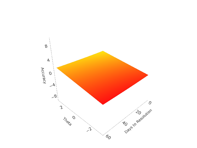
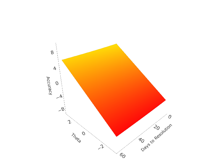
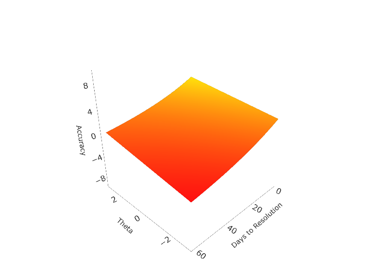
Rulison, 2010). Figure 2 presents hypothetical item response functions
based on this model. By varying b0 and b1, we illustrate
different ways forecast timing can affect accuracy; and by varying
λj we illustrate how questions with higher factor loading better discriminate forecaster ability. The slopes of the response surface illustrate the relative sensitivity of accuracy to the two factors, time and ability, in the various cases.
We also consider two additional approaches to direct skill assessment. The first variation, simple standardized accuracy, standardizes forecasters’ mean accuracy within each question, to account for differences in difficulty across questions. This is the most similar metric to what Mellers et al. (2015a) and Bo et al. (2017) used as a criterion. The key difference in our approach is that, rather than standardizing Brier scores, we standardize the normalized accuracy scores (eq. 7). This serves to both help satisfy subsequent modeling assumptions and allow for more direct comparison with the IRT approach.
The second approach accounts for the effect of time on direct skill assessment by employing the following hierarchical model:
|
Normalized Accuracyij=γ 00+µ i0+µ 0j+γ
1jlog(tij)+eij
(9) |
In this model, µi0 serves the same function as the T term in the CCT model (eq 1): an estimated forecaster-specific “true score”. However, in addition to error, in this model µi0 is also conditional on log(time) for each forecast, as well as µ0j, which represents the average accuracy of each question, across all forecasters. This effectively accounts for the difficulty (or more precisely, easiness) of each question. As such, µi0 is an estimated mean forecaster accuracy which accounts for both question difficulty and the effect of time. This model represents a compromise between the IRT and simple standardized approaches, in that it estimates fewer parameters and is more computationally efficient than the IRT approach, but still includes adjustments for question difficulty and the effect of time.
Metric Scales. The three metrics are on slightly different, but similar scales. The simple and hierarchical ability assessments are based on the actual normalized accuracy scale. Because question difficulty is accounted for, an average forecaster would be expected to have a score of 0 on both metrics, with better forecasters having higher scores and weaker forecasters having lower scores, though the units do not have a clear intuitive interpretation. On the other hand, the IRT model requires θ to be scaled for model identification. This makes the resulting metric more meaningful, as it is interpretable as estimated z-scores. This is an advantage of the IRT approach.
 |  |
| b0 = −0.5, b1 = 0.5, λ = 0.5 | b0 = −0.5, b1 = 0.5, λ = 2 |
 | 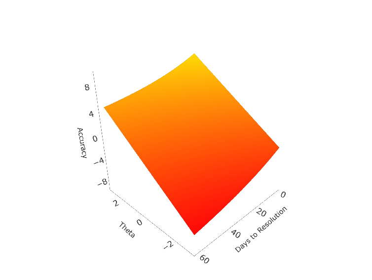 |
| b0 = −4, b1 = 4, λ = 0.5 | b0 = −4, b1 = 4, λ = 2 |
| Figure 2: Four hypothetical item response functions. Top row represents questions where difficulty is relatively constant over time, bottom row where difficulty is very sensitive to timing. Left column represents questions which poorly discriminate forecasters of differing ability levels, right column represents questions which discriminate forecasters of differing abilities well (Note that b2 is held constant at 6.63, the empirical estimate for Season 1). |
Programming. All data analysis was performed with the R statistical computing platform (R Core Team, 2020). Hierarchical models were fit with the lme4 package (Bates et al., 2015). Item response models were programmed in Stan (Stan Development Team, 2020b) and interfaced via RStan (Stan Development Team, 2020a). All programs are available in the supplementary materials.
2.2 Results and Discussion
Individual Differences. We began by probing the results of each intake scale on the data obtained from the supplementary sample (n = 1,380). Cronbach’s α ranged between moderate and good for the Cognitive Reflection Test (.80), Berlin Numeracy (.70), Number Series (.73), and Need for Cognition (.85); moderate for Matrix Reasoning (.56) and Actively Open-Minded Thinking (.64) and low for Political Knowledge (.44)4. Measurement model results for intelligence and cognitive style based on these scales are in the supplementary materials.
We removed one item from the Political Knowledge quiz because all participants answered it correctly. Overconfidence scores for the remaining 49 items in the core sample (n = 326) had mean = 0.02, SD = 0.09, where a score of 0 denotes perfect calibration, positive scores reflect over-confidence, and negative scores under-confidence. We consider forecasters who were within half a standard deviation from 0 as relatively well calibrated, forecasters who were more than half a standard deviation above 0 as over-confident, and those who were more than half a standard deviation below 0 as under-confident. We found that 133 (41%) were well-calibrated, 127 (39%) were overconfident, and only 66 (20%) were under-confident. Overall, participants were twice as likely to be overconfident than under-confident, a result which is a typical finding (Brenner et al., 1996).
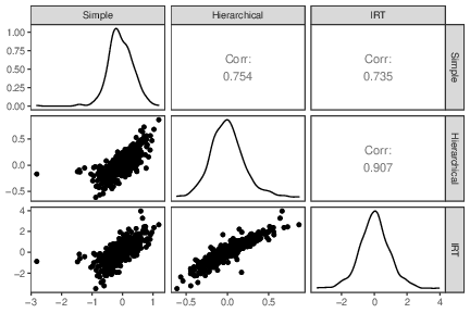
Ability Measures. Figure 3 displays the distributions and correlations between the 3 ability measures (simple, hierarchical, IRT). The three accuracy measures were highly correlated across the full dataset (326 forecasters and 188 questions). We next split the data into two halves (the first 94 questions to resolve, and the remaining 94), to test the temporal stability of these metrics. Table 2 contains correlations for each measure between and within time periods. These results are consistent with Hypothesis 2, that empirical assessments of forecaster ability based on accuracy are stable over time.
| Table 2: Correlations between accuracy measures between and within two sets of 94 forecasting questions from Season 1 (N = 326 forecasters). Between time correlations in italics, with comparisons of the same metric across time in bold. |
| | | T1 | T2 |
| | | Simple | Hierarchical | IRT | Simple | Hierarchical |
| 2[2]*T1 | Hierarchical | .72 | | | | |
| | IRT | .71 | .83 | | | |
| 3[1]*T2 | Simple | .36 | .34 | .38 | | |
| | Hierarchical | .29 | .40 | .41 | .82 | |
| | IRT | .30 | .39 | .36 | .79 | .92 |
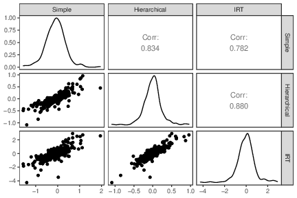
| Figure 3: Scatterplot matrix of three ability assessments (simple, hierarchical, IRT) across all forecasters from Season 1 (n = 326). |
Individual Differences Predict Estimated Ability. Table 3 displays the correlations between the ability measures and various scales and the demographic variables. As in Mellers et al. (2015a), variables related to general intelligence, cognitive style, domain knowledge, and education show the highest correlations with ability. Overall, the correlational pattern is consistent with these past findings for each of the ability measures, with some minor differences. For example, in our results, CRT, rather than matrix reasoning, shows the highest correlation with ability. However, Mellers et al. (2015a) used mean standardized Brier scores, not normalized accuracy, and accounted differently for forecast timing. It is possible that these methodological differences account for some of these minor discrepancies.
| Table 3: Correlations between measures of individual differences and accuracy (Season 1, n = 326) |
| | Simple | Hierarchical | IRT |
| Intelligence | .20 | .22 | .21 |
| Number Series | .15 | .18 | .17 |
| Berlin Numeracy | .15 | .16 | .15 |
| Cognitive Reflection Test | .20 | .22 | .20 |
| Matrix Reasoning | .15 | .10 | .11 |
| Cognitive Style | .13 | .14 | .10 |
| Actively Open-Minded Thinking | .15 | .20 | .18 |
| Need for Cognition | .15 | .17 | .14 |
| Political Knowledge (% Correct) | .11 | .11 | .09 |
| Political Knowledge (Overconfidence) | -.15 | -.13 | -.15 |
| Age | -.07 | -.05 | -.10 |
| Gender (0 = Male, 1 = Female) | .06 | .11 | .09 |
| Education | .13 | .17 | .13 |
Individual Differences Predict Accuracy. To demonstrate the relationship between individual differences and forecast accuracy, we fit a hierarchical model with intelligence, cognitive style, political knowledge, overconfidence, age, gender, and education predicting the normalized accuracy scores for each forecast, with random intercepts for forecasters and questions, and controlling for (the log of) time remaining until resolution. We compared this model to a simplified (nested) model with only these random intercepts and the time covariate. A likelihood ratio test revealed individual differences significantly predict normalized accuracy beyond the effect of time (χ2(7) = 35.11, p < .001, R2 = .14, where R2 is based on the reduction in forecaster random intercept variance attributable to individual differences using the procedure outlined by Raudenbush & Bryk, 2002). These results are consistent with Hypothesis 1¸ that individual differences predict forecast accuracy.
To understand the contributions of the individual predictors in the hierarchical model, we used dominance analysis (Budescu, 1993; Luo & Azen, 2013), a method which compares the contributions of all the predictors in all nested regression subsets to obtain a global contribution weight on the R2 scale. Results revealed that education, intelligence, and cognitive style explained the bulk of the variance in forecast accuracy (see Table 4 for full results), and that each of these factors was positively associated with accuracy.
| Table 4: Global Dominance measures of hierarchical regression of normalized accuracy on individual differences (Season 1 core volunteer sample, n = 326). |
| | Dominance Weight | % of Total R2 |
| Education | .063 | 44.3 |
| Intelligence | .029 | 21.1 |
| Cognitive Style | .026 | 18.6 |
| PK Overconfidence | .010 | 6.8 |
| PK Score | .007 | 5.1 |
| Gender | .006 | 4.1 |
| Age | <.001 | 0.0 |
| R2 = .14 | |
Explained Accuracy Over Time. Our goal is to understand how two sources of information — individual differences and past performance — predict forecast accuracy, and how they complement each other over time as more information on past performance becomes available. To accomplish this, we sorted the questions by the date they were resolved and estimated eight ability scores in intervals of 10 questions up to 80 (so each forecaster had scores based on the first 10 questions to resolve, the first 20 questions … until 80 questions). This procedure was repeated for simple, hierarchical, and IRT ability scores.
At each time point, we fit hierarchical models which predicted the normalized accuracy of the forecasts on the remaining unresolved questions (81-188) using three performance-based variables (ability score, total number of forecasts made, total unique questions forecasted), individual difference results (intelligence, cognitive style, PK quiz score, PK calibration confidence), and demographic information (age, gender, education). The models also contained random intercepts for person and question (the hierarchical portion of the model), and controlled for (the log of) time remaining to question resolution. To balance the sample of forecasters in each model, we subsetted the data further so that each model included only forecasters who made at least one forecast on the questions from first partition (n = 216 forecasters).
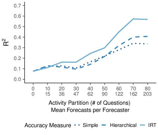
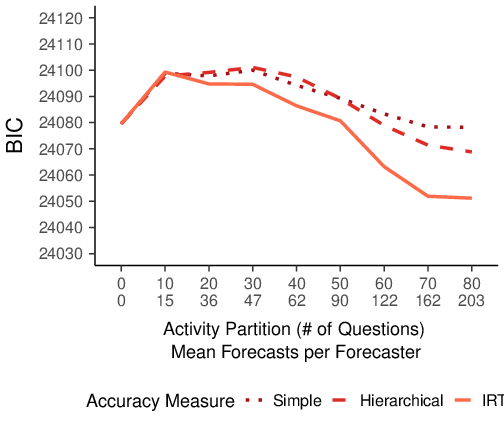
Figure 4 provides a direct comparison of the three approaches to past accuracy measurement. It displays R2 based on reduction in the participant random intercept variance attributable performance, individual differences, and demographics (Raudenbush & Bryk, 2002) and the BIC of each model. When no past performance data was available, the models contained fewer parameters, so the increase in BIC between 0 and 10 questions suggests the extra information was not immediately worth the tradeoff with reduced parsimony.
| Figure 4: Comparison of model fit (left: R2, right: BIC) for various accuracy measures, based on past performance over time (Season 1). Mean forecasts per forecaster at each time point are also displayed for reference on the X-axis (n = 216). |
When relatively few questions had resolved, the models performed similarly. However, over time, the IRT based model showed an increasingly better fit than the models based on direct ability assessment methods. When the information about all 80 questions became available, the IRT assessment-based model produced R2 = .57, the hierarchical assessment-based model R2 = .41, and the simple assessment-based model R2 = .34. These results are consistent with Hypothesis 3, that IRT ability measurement are best predictors of future accuracy, and Hypothesis 4, that including adjustments for forecast timing improves direct accuracy assessment methods. For simplicity, and because the remaining results in this section do not meaningfully differ across the three approaches, we will focus on results from the IRT models (parallel plots for hierarchical and simple accuracy models are included in the supplementary materials).
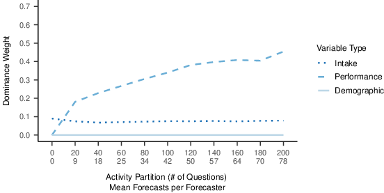
We conducted a dominance analysis on each model, so the importance of each set of predictors could be compared at each time point. Figure 5 breaks down the results at each time point by variable class: individual differences (intelligence, cognitive style, political knowledge total score, political knowledge overconfidence), past performance (ability estimates and activity levels), and demographics (age, gender, education). Although individual differences were helpful predictors early on, past performance information dominated when as few as 20 questions had resolved, and continued to explain additional variability through 80 questions (Figure 5). These results provide evidence for Hypothesis 5, that as performance information becomes available it dominates individual differences as predictors of future accuracy.
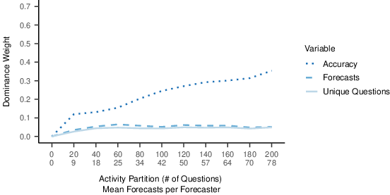
Given the dominance of performance information once it becomes available, we plotted the relative contributions of ability estimates and activity levels as well (Figure 6). Interestingly, it was the number of total forecasts that was the best predictor of future accuracy when performance information was available for fewer than 40 questions. Note that because total unique questions forecasted was also included as a separate variable, the unique contribution of total forecasts is at least partially driven by the number of times forecasters repeatedly forecasted the same questions, or put another way, updated their beliefs. As such, this result is consistent with findings that frequent belief updating is a meaningful predictor of future accuracy (Atanasov et al., 2020). When past performance information exceeded 40 questions, estimated ability surpassed total forecasts as the best predictor, though total forecasts remained a stable predictor as well (it did not trade off as accuracy information accumulated).
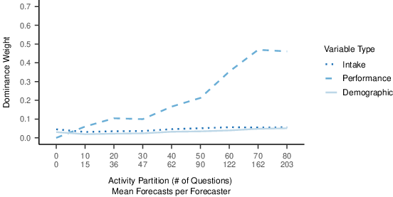
| Figure 5: Global dominance measures of different sources of information on accuracy of future forecast as a function of time, with IRT used for ability assessment (Season 1, n = 216). Mean forecasts per forecaster at each time point are also displayed for reference on the X-axis. |
Out-of-Sample Analysis. One of the main benefits of identifying skilled forecasters is to up-weight them when forecasting new questions. Our final analysis demonstrates the efficacy of these results in predicting new results from out-of-sample data, and applying them as WoC aggregation weights. Figure 4 and 5 show that the predictive value of estimated ability appears to increase as information accumulates, but the BIC results suggest it does not clearly benefit model fit until 60 questions had resolved (Figure 4B). Thus, we used the first 60 questions as calibration data, to generate ability level estimates. We partitioned the remaining 128 questions into a training set (64 questions, 61–124) and testing set (64 questions, 125–188). The training set was used as the dependent side of a series of hierarchical models with performance results from the calibration data as well as individual difference measures as predictors. Predicted estimates from these models were compared with results from the testing set (n = 202 forecasters) in two ways.
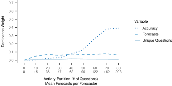
| Figure 6: Global dominance measures of different sources of past performance information on accuracy of future forecasts over time, using IRT for past ability assessment (Season 1, n = 216). Mean forecasts per forecaster at each time point are also displayed for reference on the X-axis. |
First, we fit a hierarchical model based on eq. 9 on the testing data, and compared the estimated forecaster intercepts (µi0) to the predicted results from the models fit on the training sample. Correlations between predicted estimates from the training sample and obtained estimates from the testing sample are shown in Table 5. Tests of dependent correlations (Lee & Preacher, 2013; Steiger, 1980) revealed that correlations between testing sample estimates and training sample results did not significantly differ between IRT and hierarchical assessment methods, whether individual differences were included or not. However, both methods showed significantly higher correlation with testing sample estimates than results trained with the simple method. These results provide partial evidence for Hypothesis 3, suggesting the hierarchical approach may be comparable to the more sophisticated IRT approach in an out-of-sample predictive validation, and are consistent with Hypothesis 4, that accounting for timing will benefit direct assessment.
| Table 5: Correlations between model-predicted results from training sample and observed results from testing sample by model input type (first column); cross-correlations across models in training sample (below diagonal), and absolute z-scores for tests of dependent correlations with testing sample estimates (above diagonal with significant differences at p < .05 highlighted; Lee & Preacher, 2013) from Season 1 (n = 202 forecasters, 64 questions in both testing and training samples). |
| | 2* | 3* | Training Sample Results |
| | | | With ID | Without ID |
| | | | | ID Only | Sim | Hier | IRT | Sim | Hier | IRT |
| 7* | 4*With ID | ID Only | .22 | - | 1.96 | 2.73 | 3.36 | 0.70 | 1.66 | 2.30 |
| | | Sim | .30 | .82 | - | 2.16 | 2.91 | 0.38 | 1.02 | 1.80 |
| | | Hier | .35 | .75 | .94 | - | 1.76 | 1.31 | 0.22 | 1.16 |
| | | IRT | .39 | .71 | .89 | .94 | - | 2.03 | 0.62 | 0.48 |
| | 3*Without ID | Sim | .28 | .19 | .69 | .68 | .66 | - | 2.19 | 2.99 |
| | | Hier | .36 | .19 | .60 | .76 | .72 | .85 | - | 1.64 |
| | | IRT | .41 | .20 | .56 | .68 | .79 | .78 | .89 | - |
| Note: ID = Individual Differences, Sim = Simple Accuracy, Hier = Hierarchical |
| Accuracy, IRT = IRT Accuracy |
|
Aggregation Analysis. Next, we ranked the forecasters according to their predicted skill estimates based on the training data, and used these rankings as weights in a WoC aggregation analysis for the testing data. Table 6 displays these results. The first column contains mean daily Brier scores, which was the criterion for the HFC competition, and the second column is the mean normalized accuracy.
| Table 6: Accuracy of wisdom-of-crowds weighted aggregations, by weighting input type (rows) and accuracy measure (columns) from Season 1 (n = 202 forecasters, 64 questions). |
| | | | | Mean Daily |
| Normalized |
| Accuracy |
|
| | Unweighted | 0.271 | 0.450 |
| 4* | ID Only | 0.239 | 0.547 |
| | Simple | 0.242 | 0.550 |
| | Hierarchical | 0.242 | 0.552 |
| | IRT | 0.236 | 0.568 |
| 3* | Simple | 0.251 | 0.515 |
| | Hierarchical | 0.240 | 0.564 |
| | IRT | 0.238 | 0.556 |
| Note: Higher Brier scores denote worse performance, |
| while higher normalized accuracy scores denote |
| better performance. ID = Individual Differences. |
|
Hierarchical one-way ANOVA on the normalized accuracy scores revealed the effect of weighting scheme was significant (F(7, 48169) = 260.13, p < .001). Table 7 contains pairwise contrasts with Tukey’s HSD adjustment. Results revealed that each weighted method was a significant improvement over the unweighted method, with Cohen’s d ranging from 0.09 to 0.16. However, although other results were statistically significant, the practical significance appears much smaller. For example, only IRT accuracy significantly benefited the weighting above and beyond individual differences, and Cohen’s d was only 0.02. Additionally, the IRT and hierarchical methods both improved on the simple method, with Cohen’s d values of 0.07 and 0.06, respectively; but the difference between the two was not significant.
| Table 7: Pairwise contrasts between weighting schemes on mean daily normalized accuracy from Season 1 (n = 202 forecasters, 64 questions). Positive Cohen’s d values favor alternative model. |
| Baseline Model | Alternative Model | d | t | p | 95% CI |
| 7*Unweighted | 3*No ID | Simple | 0.09 | 19.07 | <.001 | 0.08 | 0.10 |
| | | Hierarchical | 0.15 | 33.46 | <.001 | 0.14 | 0.16 |
| | | IRT | 0.14 | 31.2 | <.001 | 0.13 | 0.15 |
| | 4*With ID | ID Only | 0.13 | 28.55 | <.001 | 0.12 | 0.14 |
| | | Simple | 0.13 | 29.39 | <.001 | 0.12 | 0.14 |
| | | Hierarchical | 0.14 | 29.82 | <.001 | 0.13 | 0.14 |
| | | IRT | 0.16 | 34.46 | <.001 | 0.15 | 0.17 |
| 6*ID Only | 3*No ID | Simple | -0.04 | -9.48 | <.001 | -0.05 | -0.03 |
| | | Hierarchical | 0.02 | 4.91 | <.001 | 0.01 | 0.03 |
| | | IRT | 0.01 | 2.65 | .138 | 0.00 | 0.02 |
| | 3*With ID | Simple | 0.00 | 0.84 | .991 | -0.01 | 0.01 |
| | | Hierarchical | 0.01 | 1.27 | .910 | 0.00 | 0.01 |
| | | IRT | 0.03 | 5.91 | <.001 | 0.02 | 0.04 |
| 5* | 2*No ID | Hierarchical | 0.07 | 14.39 | <.001 | 0.06 | 0.07 |
| | | IRT | 0.06 | 12.13 | <.001 | 0.05 | 0.06 |
| | 3*With ID | Simple | 0.05 | 10.32 | <.001 | 0.04 | 0.06 |
| | | Hierarchical | 0.05 | 10.75 | <.001 | 0.04 | 0.06 |
| | | IRT | 0.07 | 15.4 | <.001 | 0.06 | 0.08 |
| 4* | 2*No ID | Hierarchical | 0.02 | 4.07 | .001 | 0.01 | 0.03 |
| | | IRT | 0.01 | 1.81 | .613 | 0.00 | 0.02 |
| | 2*With ID | Hierarchical | 0.00 | 0.43 | >.999 | -0.01 | 0.01 |
| | | IRT | 0.02 | 5.07 | <.001 | 0.01 | 0.03 |
| 3* | No ID | IRT | -0.01 | -2.26 | .318 | -0.02 | 0.00 |
| | 2*With ID | Hierarchical | -0.02 | -3.64 | .007 | -0.03 | -0.01 |
| | | IRT | 0.00 | 1.01 | .973 | 0.00 | 0.01 |
| 2* | No ID | IRT | 0.01 | 1.38 | .867 | 0.00 | 0.02 |
| | With ID | IRT | 0.02 | 4.64 | <.001 | 0.01 | 0.03 |
| IRT (No ID) | With ID | IRT | 0.01 | 3.26 | .024 | 0.01 | 0.02 |
These results provide partial evidence for Hypothesis 6. There appear to be modest benefits to aggregation weights that adjust for forecast timing in ability estimates and include individual differences. However, it is not clear that there is a practical difference between the hierarchical and IRT assessment approaches. The key takeaway appears to be that most of the benefit comes from having some method of differentiating skilled from unskilled forecasters, with only marginal gains from more sophisticated methods.
3 Study 2: HFC Season 2
The second season of HFC took place between April and November of 2019. We repeated most of the analyses with these data with a special emphasis on three questions. First, we wanted to gauge if there is a meaningful benefit to the IRT approach to skill assessment. While this model produced the best fit in Season 1, correlations with out-of-sample accuracy, and aggregation weights, gains were not significantly higher than the hierarchical assessment approach. In the aggregation analysis, the IRT and hierarchical approaches produced significantly more accurate aggregate forecasts, but the effect sizes over less sophisticated weighting methods were small, also raising questions about practical benefits. Could the data from Season 2 help clarify these results?
Second, although individual differences explained significant variability in forecast accuracy, there was an obvious cost. The battery of measures administered during Season 1 was relatively long and quite demanding, consisting of 106 individual items spread across 7 different scales. Administering such a battery is impractical in some settings. Is it possible to achieve similar results with a shorter battery?
Finally, Season 1 of the HFC recruited volunteer participants who were intrinsically motivated. Presumably, these volunteers were interested in forecasting geopolitical events. Their engagement level was self-determined, and they did not receive compensation for their efforts beyond bragging rights for accuracy. Season 2 recruited participants using Amazon Mechanical Turk. They were paid for their time, and as a result had much more homogenous levels of engagement. These recruits were, presumably, more extrinsically motivated. This population is different not only from Season 1, but from the participants from the ACE data, on which much of the past research on the psychology of forecasting is based. Would Season 1 results generalize to this new population?
3.1 Methods
Many of the methods applied to Season 2 were identical to those of Season 1. Therefore, we highlight the key differences rather than repeating information provided previously.
Sample Information. Instead of volunteers, Season 2 of the HFC recruited forecasters from Amazon Mechanical Turk via third-party firm TurkPrime (Litman et al., 2017). The sample consisted of 547 forecasters, 229 (42%) women, with a mean age of 36.68 (SD = 10.88). Forecasters were invited back at weekly intervals for forecasting sessions, in which they were required to make at least five forecasts per session to earn their compensation. As a result, there was no need to select high activity forecasters, as we did in Season 1.
One of the goals for HFC Season 2 was to establish scalability with regard to the number of forecasting questions. Season 2 had 398 questions, more than twice as many as Season 1. Questions had a mean duration of 87.07 days (SD = 55.85 days), and otherwise followed the same structure as questions from Season 1. The mean number of unique questions forecasted by every participant was 54.97 (SD = 24.32). The mean number of revisions forecasters made per question was 2.45 (SD = 2.04). A list of all forecasting questions from Season 2 is provided in the supplementary materials.
Individual Differences. We retained two scales for intelligence (Number Series, Berlin Numeracy) and one scale for cognitive style (Actively Open-Minded Thinking). We also created a shorter version of the Political Knowledge quiz by selecting 15 items to cover a range of subjects and geographic regions. The result was a battery of 36 items across four scales. The order of the 4 scales was randomized.5 Because we no longer had out-of-sample data to fit measurement models, as well as fewer scales, we used raw scale scores for all analyses.
3.2 Results
Individual Differences. Cronbach’s α was moderate for Number Series (.77) and Berlin Numeracy (.66), and surprisingly low for Actively Open-Minded Thinking (.24) and Political Knowledge (0). Despite the low reliabilities we included all the scales in subsequent analyses to facilitate comparisons with Season 1 analysis. On average, participants were more overconfident on the Political Knowledge quiz in Season 2 (Mean overconfidence = 0.15 with SD = 0.15). Using the criteria used in Season 1, 26 participants (6%) were classified as underconfident, 127 (27%) were well calibrated, and the vast majority (310, or 67%) were overconfident (84 participants did not complete the scale).
Ability Measures. Figure 7 shows the distributions and correlations between ability measures. The three measures were highly correlated across the full dataset (547 forecasters and 398 questions). We split the data into two halves (the first section contained the first 199 questions to resolve). Table 8 analyzes the temporal stability the accuracy metrics, by correlating the measures between and within time periods. These results are consistent with Hypothesis 2, that empirical assessments of forecaster ability are stable over time.
| Figure 7: Scatterplot matrix of three ability assessments (simple, hierarchical, IRT) across all from Season 2 (n = 547). |
| Table 8: Correlations between accuracy measures between and within two sets of 94 forecasting questions from Season 2 (n = 547 forecasters). Between time correlations in italics, with comparisons of the same metric across time in bold. |
| | | T1 | T2 |
| | | Simple | Hierarchical | IRT | Simple | Hierarchical |
| 2*T1 | Hierarchical | .70 | | | | |
| | IRT | .63 | .84 | | | |
| 3*T2 | Simple | .54 | .49 | .51 | | |
| | Hierarchical | .49 | .60 | .63 | .69 | |
| | IRT | .53 | .62 | .66 | .72 | .90 |
Individual Differences Predict Ability and Accuracy. Table 9 shows the correlations between individual difference scales and ability measures. A hierarchical model controlling for (the log of) time remaining to resolution, with random intercepts for question and forecaster, revealed individual difference variables jointly predicted the accuracy of forecasts (χ2(8) = 52.24, p < .001, R2 = .11. ). The dominance analysis results are displayed in Table 10.
| Table 9: Correlations between individual differences and accuracy (Season 2, n = 547). |
| | Simple | Hierarchical | IRT |
| Number Series | .30 | .30 | .30 |
| Berlin Numeracy | .28 | .23 | .25 |
| Actively Open-Minded Thinking | .00 | .04 | .02 |
| Political Knowledge (% Correct) | .10 | .10 | .11 |
| Political Knowledge (Overconfidence) | −.14 | −.13 | −.14 |
| Age | .06 | .04 | .03 |
| Gender | −.04 | −.05 | −.08 |
| Education | −.03 | −.04 | −.08 |
| Table 10: Global dominance measures of hierarchical regression of normalized accuracy on individual differences (Season 2, n = 547) |
| | Dominance Weight | % of Total R2 |
| Intelligence | .063 | 56.4 |
| Cognitive Style | .030 | 26.7 |
| Age | .015 | 13.2 |
| PK Overconfidence | .003 | 3.1 |
| PK Score | <.001 | 0.0 |
| Gender | <.001 | 0.0 |
| Education | <.001 | 0.0 |
While these results are generally consistent with Season 1 and Mellers et al. (2015a), a few key differences stand out. The Actively Open-Minded Thinking and Political Knowledge scales were less predictive in this sample, possibly due to poor reliability. More importantly, education is no longer a meaningful predictor of accuracy in these data. This is likely due to low
variability: only 11% of the MTurkers had at least a bachelor’s degree. These results support Hypothesis 1, that individual differences will predict accuracy.
Explained Accuracy Over Time. We generated ability scores for all participants at a number of intervals based on performance in the first half of the Season. Because there were more questions, we calculated 10 different longitudinal scores using intervals of 20 questions (based on 0, 20, 40….200 questions). We used those ability estimates along with individual differences and demographics to build models to predict accuracy on the final 198 questions. We only used those participants who forecasted at least one question among the first 20 and the final 198 questions to match the sample sizes across models (n = 409).
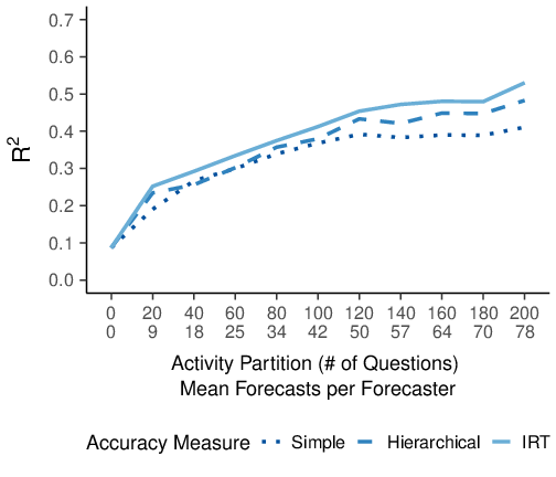
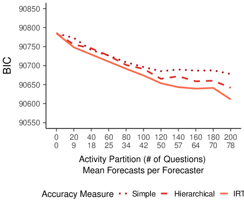
Figure 8 is similar to Figure 4 from Season 1, comparing overall R2 and BIC by accuracy measurement approach over time. As in Season 1, the IRT model performed best, but the differences between measures were small. With performance information on 200 questions, the IRT assessment approach produced R2 = .53, the hierarchical assessment approach produced R2 = .48, and the simple assessment approach produced R2 = .41. In this sample, the model fits improved more slowly compared to Season 1. For example, the IRT assessment model had R2 = .35 when 80 questions had resolved in Season 2, compared to R2 = .57 in Season 1 when 80 questions had resolved. This is likely due to the reduced number of forecasts per question at each time point, a function of the higher density of questions. On the other hand, BIC did not initially increase when performance measures were added in Season 2, suggesting they provided more immediate benefit compared to Season 1. We again focus on the IRT approach, with alternative plots in the supplementary materials.
| Figure 8: Comparison of model fit (left: R2, right: BIC) for three accuracy measures based on past performance as a function of time (Season 2, n = 409). Mean forecasts per forecaster at each time point are also displayed for reference on the X-axis. |
We conducted a dominance analysis on each model, so the importance of each set of predictors could be compared at each time point. Figure 9 breaks down the results at each time point by variable class: individual difference measures, past performance, and demographics. Results are consistent with Season 1, in that past performance information dominated when only 20 questions had resolved, and continued to improve through 80 questions. Figure 10 plots the contributions of each performance variable (ability estimate, total forecasts, unique questions). Unlike Season 1, ability estimates were the dominant performance-based predictor as soon as they became available. The reduced predictive utility of past activity is possibly due the reduced variability in engagement levels among the MTurkers in Season 2 as compared to the volunteers in Season 1. These results are consistent with Hypothesis 5, that past performance information would be the dominant predictor of future accuracy as it accumulates.
| Figure 9: Global dominance measures of different sources of information on accuracy of future forecast as a function of time, with IRT used for ability assessment (Season 2, n = 409). Mean forecasts per forecaster at each time point are also displayed for reference on the X-axis. |
| Figure 10: Global dominance measures of different sources of past performance information on accuracy of future forecasts over time, using IRT for past ability assessment (Season 2, n = 409). Mean forecasts per forecaster at each time point are also displayed for reference on the X-axis. |
Out-of-Sample Analysis. In Season 2, we used the first 150 questions to calibrate accuracy metrics, the next 150 to train predictive models, and the final 98 to test model predictions (n = 391 forecasters across all three samples). We began by comparing training data model predictions to µi0 values obtained from the testing sample. The IRT and Hierarchical accuracy approaches produced virtually identical correlations with estimated testing sample accuracy (Table 11), but again performed significantly better than the simple accuracy measure, as well as individual differences alone, by tests of dependent correlation (Lee & Preacher, 2013; Steiger, 1980). These results partially support Hypothesis 3 (the IRT method will perform better than others) and support Hypothesis 4 (accounting for timing will benefit direct assessment). They are also highly consistent with Season 1 results, suggesting that the IRT and hierarchical methods of ability measurement perform better than the simple method or individual differences alone.
| Table 11: Correlations between model-predicted results from training sample and observed results from testing sample, by model input type; and cross-correlations across models in training sample (first column); cross-correlations across models in training sample (below diagonal), and absolute z-scores for tests of dependent correlations with testing sample estimates (above diagonal with significant differences at p < .05 highlighted; Lee & Preacher, 2013)from Season 2 (n = 391, 150 training questions, 98 testing questions). |
| | 2* | 3* | Training Sample Results |
| | | | With ID | Without ID |
| | | | | ID Only | Sim | Hier | IRT | Sim | Hier | IRT |
| 7* | 4*With ID | ID Only | .21 | − | 5.88 | 7.38 | 7.24 | 5.06 | 6.59 | 6.50 |
| | | Sim | .48 | .50 | − | 2.64 | 2.17 | 0.00 | 2.74 | 2.25 |
| | | Hier | .54 | .50 | .86 | − | 0.00 | 2.33 | 0.96 | 0.43 |
| | | IRT | .54 | .48 | .79 | .88 | − | 1.99 | 0.44 | 0.96 |
| | 3*Without ID | Sim | .48 | .32 | .96 | .82 | .75 | − | 2.99 | 2.38 |
| | | Hier | .55 | .32 | .82 | .97 | .85 | .85 | − | 0.00 |
| | | IRT | .55 | .30 | .73 | .84 | .97 | .76 | .87 | − |
| Note: ID = Individual Differences, Sim = Simple Accuracy, Hier = Hierarchical |
| Accuracy, IRT = IRT accuracy |
|
Aggregation Analysis. We tested the utility of each measurement approach in WoC aggregation across the testing sample questions. The effect of weighting method on mean daily normalized accuracy was again significant in a hierarchical one-way ANOVA with random intercepts for question (F(7, 78567) = 122.46, p < .001). Table 12 shows the mean daily Brier and Normalized Accuracy scores. Table 13 shows pairwise contrasts with Tukey HSD adjustment. Results are largely consistent with Season 1, in that the largest differences were in comparisons involving unweighted aggregates. This confirms that there is a benefit to weighting forecasters by estimated ability, but that more sophisticated methods of measuring ability provide only marginal benefits. There were also a few key differences. In Season 1, there was a clear benefit to the IRT and hierarchical approaches over the simple ability assessment. This benefit is less clear in Season 2; in fact, none of the differences between models that included ability estimates were significantly different from one another. However, in Season 2, there was a larger benefit to including accuracy above and beyond individual differences. Overall, the Season 2 results fail to support Hypothesis 6, that IRT accuracy measurement will optimize WoC aggregation weights when compared to other methods of ability assessment. Although the correlational results suggest the IRT (and hierarchical) approaches better discriminate the skill of individual forecasters, this does not appear to benefit WoC aggregation in Season 2 over simpler methods of ability assessment. It is possible that there are diminishing returns on the increased methodological sophistication in WoC aggregation, or that different aggregation methods might be more sensitive to these differences.
| Table 12: Accuracy of wisdom-of-crowds weighted aggregations, by weighting input type (rows) and accuracy measure (columns) from Season 2 (n = 391 forecasters, 98 questions). |
| | | | | Mean Daily |
| Normalized |
| Accuracy |
|
| | Unweighted | 0.339 | 0.419 |
| 4* | ID Only | 0.331 | 0.454 |
| | Simple | 0.325 | 0.482 |
| | Hierarchical | 0.325 | 0.482 |
| | IRT | 0.325 | 0.482 |
| 3* | Simple | 0.323 | 0.484 |
| | Hierarchical | 0.324 | 0.489 |
| | IRT | 0.324 | 0.491 |
| Note: Higher Brier scores denote worse performance, |
| while higher normalized accuracy scores denote |
| better performance. ID = Individual Differences. |
|
| Table 13: Pairwise contrasts between weighting schemes on mean daily normalized accuracy from Season 2 (n = 391 forecasters, 98 questions). Positive Cohen’s d values favor alternative model. |
| Baseline Model | Alternative Model | d | t | p | 95% CI |
| 7*Unweighted | 3*No ID | Simple | 0.07 | 20.59 | <.001 | 0.07 | 0.08 |
| | | Hierarchical | 0.08 | 21.05 | <.001 | 0.07 | 0.08 |
| | | IRT | 0.08 | 22.77 | <.001 | 0.07 | 0.09 |
| | 4*With ID | ID Only | 0.04 | 11.01 | <.001 | 0.03 | 0.05 |
| | | Simple | 0.07 | 19.80 | <.001 | 0.06 | 0.08 |
| | | Hierarchical | 0.07 | 20.01 | <.001 | 0.06 | 0.08 |
| | | IRT | 0.08 | 21.95 | <.001 | 0.07 | 0.09 |
| 6*ID Only | 3*No ID | Simple | 0.03 | 9.57 | <.001 | 0.03 | 0.04 |
| | | Hierarchical | 0.04 | 10.04 | <.001 | 0.03 | 0.04 |
| | | IRT | 0.04 | 11.75 | <.001 | 0.03 | 0.05 |
| | 3*With ID | Simple | 0.03 | 8.79 | <.001 | 0.02 | 0.04 |
| | | Hierarchical | 0.03 | 9.00 | <.001 | 0.03 | 0.04 |
| | | IRT | 0.04 | 10.94 | <.001 | 0.03 | 0.05 |
| 5*Simple (No ID) | 2*No ID | Hierarchical | 0.00 | 0.46 | >.999 | −0.01 | 0.01 |
| | | IRT | 0.01 | 2.18 | .363 | 0.00 | 0.01 |
| | 3*With ID | Simple | 0.00 | −0.78 | .994 | −0.01 | 0.00 |
| | | Hierarchical | 0.00 | −0.57 | .999 | −0.01 | 0.00 |
| | | IRT | 0.00 | 1.37 | .872 | 0.00 | 0.01 |
| 4*Simple (With ID) | 2*No ID | Hierarchical | 0.00 | 1.25 | .917 | 0.00 | 0.01 |
| | | IRT | 0.01 | 2.97 | .060 | 0.00 | 0.02 |
| | 2*With ID | Hierarchical | 0.00 | 0.21 | >.999 | −0.01 | 0.01 |
| | | IRT | 0.01 | 2.15 | .381 | 0.00 | 0.01 |
| 3*Hierarchical (No ID) | No ID | IRT | 0.01 | 1.72 | .677 | 0.00 | 0.01 |
| | 2*With ID | Hierarchical | 0.00 | −1.04 | .969 | −0.01 | 0.00 |
| | | IRT | 0.00 | 0.90 | .986 | 0.00 | 0.01 |
| 2*Hierarchical (With ID) | No ID | IRT | 0.01 | 2.75 | .107 | 0.00 | 0.02 |
| | With ID | IRT | 0.01 | 1.94 | .523 | 0.00 | 0.01 |
| IRT (No ID) | With ID | IRT | 0.00 | −0.81 | .992 | −0.01 | 0.00 |
4 General Discussion
4.1 Revisiting the Research Questions
Our results provide clear support for Hypotheses 1, 2, 4, and 5, as well as partial support for Hypotheses 3 and 6. We began by confirming two established findings (Hypotheses 1 and 2): that both individual differences (Aspinall, 2010; Colson & Cooke, 2018; Hanea et al., 2018; Mellers, et al., 2015a) and past performance (Bo et al., 2017; Mellers, et al., 2015a; Mellers, et al., 2015b; Merkle et al., 2016; Tetlock & Gardner, 2016) can be used to predict the accuracy of future forecasts. We found that several sources of individual difference separately correlate with both the accuracy of forecasters’ individual forecasts as well as their aggregate performance measured in different ways. There were slight inconsistencies across the two seasons. For example, education was the dominant cold start predictor of future accuracy in Season 1 (Table 4), but it was not a helpful predictor in Season 2 (Table 10). This may be attributable to differences between the makeup of the volunteer population used in Season 1 and the MTurk population in Season 2.
Season 2 results also suggested the amount of individual difference information required to identify skilled forecasters in the absence of past performance information could be dramatically reduced with little cost to model performance through judicious choices. Season 1 featured a battery of 106 items, but with the benefit of these results, we managed to reduce the battery to only about one third in length (36 items) in Season 2, without a serious drop in its predictive validity.
We determined that, although individual differences are helpful at addressing the cold start problem, once performance data becomes available, it dominates individual differences in predictive utility (Hypothesis 5). However, it was not necessarily just past accuracy-estimates that predicted future accuracy. In Season 1, when there was higher variability in engagement levels, the total number of forecasts made was a better predictor than estimated ability when relatively little performance information was available. This is consistent with the interesting finding from Mellers et al. (2015a) and Atanasov et al. (2020) that forecasters who update their beliefs more frequently tend to be more accurate. However, once a critical mass of performance information became available in Season 1, and throughout Season 2, estimates of forecasting ability based on the accuracy of past forecasts did ultimately dominate all other predictors of future accuracy.
We demonstrated the utility of the IRT approach to modeling forecasting skill (Bo et al., 2017; Merkle et al., 2016), particularly with regard to accounting for the timing of forecasts in a setting in which forecasters can forecast the same questions repeatedly at different times (Hypothesis 3). This estimation method performed notably better than the traditional approach of averaging the accuracy of past forecasts, without accounting for the effect of time. However, we also determined that a simpler approach based on hierarchical linear modeling with a time component performed comparably to the IRT approach (Hypothesis 4). This hierarchical approach adapts the probit normalization procedure Merkle et al. (2016) used in their IRT model, but is much faster and more computationally efficient, converging on results in seconds, where the IRT models can take an hour or more, depending on computational power. Although the hierarchical model bears some resemblance to the IRT model, it more closely resembles classical test theory models.
In addition to reporting model fit statistics and effect sizes, we were able demonstrate the predictive utility of our methods on out-of-sample data. In both Season 1 and Season 2, models trained on IRT or hierarchical ability assessment had higher correlations with out-of-sample results than models based on simple ability assessment or individual differences alone. Our models also produced beneficial WoC aggregation weights that outperformed the unweighted aggregates in both seasons. However, contrary to Hypothesis 6, while there was evidence that both individual differences and past accuracy measures benefited these weights, more sophisticated methods provided surprisingly small benefits over less sophisticated methods. Most of the benefit came from simply having a valid estimate of forecasting skill. This result confirms, again, the prominence of identifying the right predictors over the estimation of the weights (e.g., Budescu & Chen, 2015; Dawes, 1979).
Despite some minor differences in the details, the results across the two seasons were remarkably consistent. This is especially important given the different populations who participated in the two seasons. Season 1 relied on uncompensated volunteers, who were presumably drawn to the prospect of participating in a forecasting tournament. This population was more similar to the forecasters who participated in the ACE program (Bo et al., 2017; Mellers et al., 2015a; Merkle et al., 2016). Season 2 used compensated Amazon Mechanical Turk workers. While this is a somewhat unique population, demonstrating that results generalize to a population engaged for compensation rather than intrinsic interest may be important for managers attempting to identify and cultivate high performing analysts in professional settings.
Although our results document only small benefits to estimating IRT models that require extra parameters at considerable computational time compared to simpler hierarchical models, measuring trait levels is not the only possible application of such models. Future research may wish to explore the properties of different forecasting questions. Is it possible to identify patterns in why certain questions tend to be more difficult than others, or how question difficulty changes over time? Are there certain questions that are particularly effective at discriminating skilled from unskilled forecasters? Such questions are beyond the scope of this research, but they may be answerable by studying estimated item parameters from the IRT models.
4.2 Contributions to Generalizability
A number of features of the HFC tournament make these results more generalizable than past work on geopolitical forecasting. The randomized controlled trial structure of the HFC was a more scientifically conducive environment than was provided by the ACE program, where forecasters had more freedom to select into preferred research platforms. Forecasters were assigned to SAGE by a random mechanism, so it is highly unlikely that features of the platform, or its reputation,6 attracted certain types of forecasters and not others.
HFC also had a wider range of questions structures; particularly with regard to the number and ordering of response options. Many past forecasting studies have focused on binary questions (Bo et al., 2017; Mellers, et al., 2015a; Mellers et al., 2014). In HFC, across the two seasons, 281 (48%) of the questions had more than two response options, and 242 (41%) had a meaningful ordering to the response options. Questions with this structure provide a unique challenge to properly evaluate with regard to accuracy. Our results are among the first to show empirically that past results about forecasting skill identification extend to these questions.
We also successfully demonstrated the effectiveness of IRT models of forecasting ability in data sets with high levels of sparsity. Bo et al. (2017) and Merkle et al. (2016) demonstrated proof of concept for these models, but did so by selecting data based on questions with a high response rate and especially active forecasters. Our results did not select questions based on response rate or highly active forecasters, and the effectiveness of these models was clear nonetheless.
4.3 Limitations
Despite these strengths, one shortcoming of this investigation is its domain specificity. The forecasting questions in the HFC were highly specialized, and occasionally idiosyncratic, calling on forecasters to do independent research about topics with which they likely lacked deep familiarity. It is an open question how well these results would generalize to other domains, particularly domains in which forecasters may have more familiarity and expertise. It seems reasonable to hypothesize that past performance would be even more informative under such circumstances, but it would be interesting to test this empirically.
Another note of caution is that several individual difference scales had weak reliabilities. Across both seasons, the main culprit was the Political Knowledge scale. As this is not a scale has not been independently validated, investigation into the existence and measurement of political knowledge as a psychological construct would be a worthwhile endeavor. In Season 2, the Actively Open-Minded Thinking scale also showed poor reliability. It is possible that a longer instrument (e.g. Stanovich & West, 1997) would have produced stronger results. However, despite these reliability-related limitations, even the short individual difference battery in Season 2 was sufficient for predicting accuracy to a meaningful extent.
Finally, although a confidence calibration metric was included in the Political Knowledge quiz for both Seasons 1 and 2, results were inconsistent with regard to its predictive utility. This was a somewhat narrow attempt to incorporate Cooke’s method (Aspinall, 2010; Colson & Cooke, 2018) for addressing the cold start problem. Future research might consider a more direct comparison between the primary individual difference assessments applied here with a more robust adaptation of Cooke’s method.
4.4 Recommendations
Our results provide benchmarks which can be applied to future settings which rely on forecasting judgments. In cases where there is a benefit to generating immediate performance weights, we recommend prioritizing assessment of forecasters in terms of intelligence, with a focus on measures of numerical reasoning (e.g. cognitive reflection, numeracy, series completion). These metrics provide clear benefit in cold start situations. Other assessment options include cognitive style, domain knowledge, and confidence calibration, though the benefits of these predictors are less clear. Even with these scales, our results indicate such an assessment can be conducted based on fewer than 40 items.
If performance weights are not required before data has begun to accumulate, we suggest focusing more on past performance: specifically, estimating forecasters’ skill based on past accuracy, as well as measures of engagement, when relevant. If computationally feasible, the IRT models described here perform similarly or better than the other methods, and also have the advantage of being on an intuitively interpretable scale (estimated z-scores). However, if faster results are required, and intuitive scaling is not a requirement, the hierarchical model provides a more computationally efficient alternative that produces comparable results.
5 Conclusion
The goal of forecasting is to provide objective estimates of the likelihood
of future events. The challenge we posed to ourselves as researchers was to
predict the accuracy of forecasts based on information about the
forecasters who made them. Our results build on past findings by showing
that different sources of information — stable individual differences and
past performance — provide complementary utility for doing just that. We
also provide novel contributions to understanding the importance the timing
of forecasts when assessing forecasters. These results add to the growing
body of literature that suggests this meta-forecasting exercise can indeed
yield improvements in applying the theory of Wisdom-of-Crowds to
forecasting future events.
References
Aspinall, W. (2010). A route to more tractable expert advice.
Nature,
463(7279), 294–295.
Atanasov, P., Rescober, P., Stone, E. R., Swift, S. A.,
Servan-Schreiber, E., Tetlock, P., Ungar, L., & Mellers, B. A. (2017).
Distilling the wisdom of crowds: Prediction markets vs. prediction
polls. Management Science, 63(3), 691–706.
Atanasov, P., Witkowski, J., Ungar, L. H., Mellers, B. A., & Tetlock,
P. E. (2020). Small steps to accuracy: Incremental belief updaters are better forecasters. Organizational Behavior and Human Decision
Processes, 160, 19–35.
Bandalos, D. L. (2018). Measurement Theory and Applications for
the Social Sciences. Guildford Press.
Baron, J., Scott, S., Fincher, K., & Metz, S. E. (2015). Why does the
Cognitive Reflection Test (sometimes) predict utilitarian moral judgment
(and other things)? Journal of Applied Research in Memory and
Cognition, 4(3), 265–284.
Barton, M. A., & Lord, F. M. (1981). An upper asymptote for the
three-parameter logistic item-response model. ETS Research
Report Series, 1981(1), i–8.
Bates, D., Mächler, M., Bolker, B., & Walker, S. (2015). Fitting linear
mixed-effects models using {lme4}. Journal of Statistical
Software, 67(1), 1–48.
https://doi.org/10.18637/jss.v067.i01.
Bo, Y. E., Budescu, D. V, Lewis, C., Tetlock, P. E., & Mellers, B. A.
(2017). An IRT forecasting model: linking proper scoring rules to item
response theory. Judgment and Decision Making, 12
(2), 90–104.
Brenner, L. A., Koehler, D. J., Liberman, V., & Tversky, A. (1996).
Overconfidence in probability and frequency judgments: A critical
examination. Organizational Behavior and Human Decision
Processes, 65(3), 212–219.
Brier, G. W. (1950). Verification of forecasts expressed in terms of
probability. Monthly Weather Review, 78(1), 1–3.
Budescu, D. V. (1993). Dominance analysis: a new approach to the problem
of relative importance of predictors in multiple regression.
Psychological Bulletin, 114(3), 542.
Budescu, D. V., & Chen, E. (2014). Identifying expertise to extract the
wisdom of crowds. Management Science, 61(2),
267–280.
Cacioppo, J. T., & Petty, R. E. (1982). The need for cognition.
Journal of Personality and Social Psychology, 42
(1), 116–131.
Chen, E., Budescu, D. V, Lakshmikanth, S. K., Mellers, B. A., &
Tetlock, P. E. (2016). Validating the contribution-weighted model:
Robustness and cost-benefit analyses. Decision Analysis,
13(2), 128–152.
Cokely, E. T., Galesic, M., Schulz, E., Ghazal, S., & Garcia-Retamero,
R. (2012). Measuring risk literacy: The Berlin Numeracy Test.
Judgment and Decision Making.
Colson, A. R., & Cooke, R. M. (2018). Expert elicitation: using the
classical model to validate experts’ judgments. Review of
Environmental Economics and Policy, 12(1), 113–132.
Davis-Stober, C., Budescu, D. V, Dana, J., & Broomell, S. (2014). When
is a crowd wise? Decision, 1(2), 79–101.
Dawes, R. M. (1979). The robust beauty of improper linear models in
decision making. American Psychologist, 34(7),
571–582. https://doi.org/10.1037/0003--066X.34.7.571.
Dieckmann, N. F., Gregory, R., Peters, E., & Hartman, R. (2017). Seeing
what you want to see: how imprecise uncertainty ranges enhance motivated
reasoning. Risk Analysis, 37(3), 471–486.
Embretson, S. E., & Reise, S. P. (2013). Item response theory
. Psychology Press.
Fan, Y., Budescu, D. V, Mandel, D., & Himmelstein, M. (2019). Improving
accuracy by coherence weighting of direct and ratio probability
judgments. Decision Analysis, 16(3), 197–217.
Frederick, S. (2005). Cognitive reflection and decision making.
Journal of Economic Perspectives, 19(4), 25–42.
Gneiting, T., & Raftery, A. E. (2007). Strictly proper scoring rules,
prediction, and estimation. Journal of the American Statistical
Association, 102(477), 359–378.
Hanea, A. M., McBride, M. F., Burgman, M. A., & Wintle, B. C. (2018).
The value of performance weights and discussion in aggregated expert
judgments. Risk Analysis, 38(9), 1781–1794.
IARPA. (2018). A next generation intelligence research project combining
human predictions and artificial intelligence. In Cultivate
Forecasts - Prediction Markets & Crowdsourced Forecasting. IARPA.
https://www.hybridforecasting.com/.
Jose, V. R. R., Nau, R. F., & Winkler, R. L. (2009). Sensitivity to
distance and baseline distributions in forecast evaluation.
Management Science, 55(4), 582–590.
Karvetski, C. W., Olson, K. C., Mandel, D. R., & Twardy, C. R. (2013).
Probabilistic coherence weighting for optimizing expert forecasts.
Decision Analysis, 10(4), 305–326.
Lee, I. A., & Preacher, K. J. (2013). Calculation for the test
of the difference between two dependent correlations with one variable
in common. http://quantpsy.org/corrtest/corrtest2.htm.
Lika, B., Kolomvatsos, K., & Hadjiefthymiades, S. (2014). Facing the
cold start problem in recommender systems. Expert Systems with
Applications, 41(4), 2065–2073.
Litman, L., Robinson, J., & Abberbock, T. (2017). TurkPrime. com: A
versatile crowdsourcing data acquisition platform for the behavioral
sciences. Behavior Research Methods, 49(2),
433–442.
Loken, E., & Rulison, K. L. (2010). Estimation of a four-parameter item
response theory model. British Journal of Mathematical and
Statistical Psychology, 63(3), 509–525.
Lord, F. M., & Novick, M. R. (1968). Statistical theories of
mental test scores. Reading, MA. Addison-Wesley Publishing Company.
Luo, W., & Azen, R. (2013). Determining predictor importance in
hierarchical linear models using dominance analysis. Journal of
Educational and Behavioral Statistics, 38(1), 3–31.
Mandel, D. R., & Barnes, A. (2014). Accuracy of forecasts in strategic
intelligence. Proceedings of the National Academy of Sciences,
111(30), 10984–10989.
Matzen, L. E., Benz, Z. O., Dixon, K. R., Posey, J., Kroger, J. K., &
Speed, A. E. (2010). Recreating Raven’s: Software for systematically
generating large numbers of Raven-like matrix problems with normed
properties. Behavior Research Methods, 42(2),
525–541.
Mellers, B. A., Baker, J. D., Chen, E., Mandel, D. R., & Tetlock, P. E.
(2017). How generalizable is good judgment? A multi-task,
multi-benchmark study. Judgment and Decision Making,
12(4), 369–381.
Mellers, B. A., Stone, E. R., Atanasov, P., Rohrbaugh, N., Emlen Metz,
S., Ungar, L., Bishop, M. M., Horowitz, M., Merkle, E., & Tetlock, P.
E. (2015). The psychology of intelligence analysis: Drivers of
prediction accuracy in world politics. Journal of Experimental
Psychology: Applied, 21(1), 1–14.
https://doi.org/10.1037/xap0000040.
Mellers, B. A., Stone, E. R., Murray, T., Minster, A., Rohrbaugh, N.,
Bishop, M. M., Chen, E., Baker, J., Hou, Y., Horowitz, M., & Others.
(2015). Identifying and cultivating superforecasters as a method of
improving probabilistic predictions. Perspectives on
Psychological Science, 10(3), 267–281.
Mellers, B., Ungar, L., Baron, J., Ramos, J., Gurcay, B., Fincher, K.,
Scott, S. E., Moore, D., Atanasov, P., Swift, S. A., & others. (2014).
Psychological strategies for winning a geopolitical forecasting
tournament. Psychological Science, 25(5),
1106–1115.
Merkle, E. C., & Steyvers, M. (2013). Choosing a strictly proper
scoring rule. Decision Analysis, 10(4), 292–304.
Merkle, E. C., Steyvers, M., Mellers, B. A., & Tetlock, P. E. (2016).
Item response models of probability judgments: Application to a
geopolitical forecasting tournament. Decision, 3
(1), 1.
Merkle, E. C., Steyvers, M., Mellers, B., & Tetlock, P. E. (2017). A
neglected dimension of good forecasting judgment: The questions we
choose also matter. International Journal of Forecasting,
33(4), 817–832.
Moore, D. A., Swift, S. A., Minster, A., Mellers, B. A., Ungar, L.,
Tetlock, P. E., Yang, H. H. J., & Tenney, E. R. (2016). Confidence
calibration in a multiyear geopolitical forecasting competition.
Management Science, 63(11), 3552–3565.
Morstatter, F., Galstyan, A., Satyukov, G., Benjamin, D., Abeliuk, A.,
Mirtaheri, M., Hossain, K. S. M., Szekely, P., Ferrara, E., Matsui, A.,
& others. (2019). SAGE: a hybrid geopolitical event forecasting system.
Proceedings of the 28th International Joint Conference on
Artificial Intelligence, 6557–6559.
Murphy, A. H. (1973). A new vector partition of the probability score.
Journal of Applied Meteorology, 12(4), 595–600.
Novick, M. R. (1966). The axioms and principal results of classical test
theory. Journal of Mathematical Psychology, 3(1), 1–18.
R Core Team. (2020). R: A Language and Environment for
Statistical Computing. https://www.r-project.org/.
Raudenbush, S. W., & Bryk, A. S. (2002). Hierarchical linear
models: Applications and data analysis methods (Vol. 1). Sage.
Raven, J. (2000). The Raven’s progressive matrices: change and stability
over culture and time. Cognitive Psychology, 41
(1), 1–48.
Schein, A. I., Popescul, A., Ungar, L. H., & Pennock, D. M. (2002).
Methods and metrics for cold-start recommendations. Proceedings
of the 25th Annual International ACM SIGIR Conference on Research and
Development in Information Retrieval, 253–260.
Stael von Holstein, C. A. (1970). Measurement of subjective probability.
Acta Psychologica, Amsterdam, 34(2–3), 146–159.
Stan Development Team. (2020a). {RStan}: the {R} interface
to {Stan}. http://mc-stan.org/
R package version 2.21.2
Stan Development Team. (2020b). Stan Modeling Language Users
Guide and Reference Manual (2.25). https://mc-stan.org.
Stanovich, K. E., & West, R. F. (1997). Reasoning independently of
prior belief and individual differences in actively open-minded
thinking. Journal of Educational Psychology, 89
(2), 342–357.
Steiger, J. H. (1980). Tests for comparing elements of a correlation
matrix. Psychological Bulletin, 87, 245–251.
Surowiecki, J. (2005). The wisdom of crowds. Anchor.
Tetlock, P. E., & Gardner, D. (2016). Superforecasting: The
art and science of prediction. Random House.
Tetlock, P. E., Mellers, B. A., Rohrbaugh, N., & Chen, E. (2014).
Forecasting tournaments: Tools for increasing transparency and improving
the quality of debate. Current Directions in Psychological
Science, 23(4), 290–295.
Wallsten, T. S., & Budescu, D. V. (1983). Encoding subjective
probabilities: A psychological and psychometric review.
Management Science, 29(2), 151–173.
Witkowski, J., Atanasov, P., Ungar, L., & Krause, A. (2017, February). Proper proxy scoring rules. In Proceedings of the AAAI Conference on Artificial Intelligence, 311. Retrieved from https://ojs.aaai.org/index.php/AAAI/article/view/10590
This document was translated from LATEX by
HEVEA.