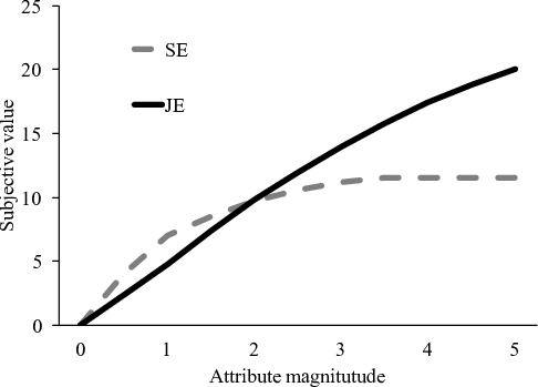
| Figure 1: Subjective value judgments of a hypothetical attribute under SE vs. JE modes (adopted from Hsee & Zhang, 2004). |
Judgment and Decision Making, Vol. 16, No. 1, January 2021, pp. 94-113
When two wrongs make a right: The efficiency-consumption gap under separate vs. joint evaluationsEyal Gamliel* Eyal Pe’er# |
Abstract: The MPG illusion and the time-saving bias both show that people misjudge the gains from increases in efficiency or speed, because people falsely believe that efficiency and speed are linearly related to consumption (e.g., gallons of fuel or journey time). This efficiency-consumption gap (ECG) has been demonstrated consistently in various situations. In parallel, people have also been found to show a diminished sensitivity to increases in magnitudes when judged under separate vs. joint evaluation modes (SE vs. JE). We show that these “two wrongs can make a right”: when people judge efficiency upgrades under SE mode, their subjective judgments follow a concave curve that closely resembles the curvilinear pattern of efficiency upgrades, making their preferences (artificially) less biased than they are under JE. In two studies we show that when asked for their willingness-to-pay (WTP) for upgrading products or services in two (a smaller vs. a larger) upgrade options, WTPs are less different in SE vs. JE modes. This means that people are exhibiting lower sensitivity to the upgrade size under SE which leads to a de-biasing effect. We show that because JE follow a linear trend, it yields biased preferences for efficiency measures, but not for consumption measures. In contrast, SE yield biased preferences for consumption, but not for efficiency measures.
Keywords: efficiency savings, time saving bias, the mpg illusion, joint and separate evaluations, evaluability theory
When it comes to judging non-linear relationships, such as how much fuel can one save when upgrading a car, or how much time can one save when increasing speed, people have been found to err consistently and considerably (e.g., Larrick & Soll, 2008; Svenson, 2008). Expansive studies, covering various examples, measures and values, have repeatedly asked people to judge the impact of a change in measures of efficiency (e.g., miles-per-gallons) or speed (e.g., Mph, km/h, Mbps) or productivity (e.g., units-per-day) on the inversely related measures of consumption (e.g., gallons-per-mile, minutes-per-mile, seconds-per-megabit, day’s units). They all found that people falsely regard the relationship between these two types of measures as if it is linear, when it is curvilinear by definition. This false assumption leads people to underestimate the impact of increases from relatively lower values of speed or efficiency and overestimate the impact of increases from relatively higher values (De Langhe et al., 2017; De Langhe & Puntoni, 2016; Eriksson et al., 2013; Peer, 2010, 2011; Peer & Gamliel, 2012, 2013; Svenson, 1970, 1973, 1976, 2008, 2009, 2011; Svenson & Borg, 2020).
For example, people falsely believe that upgrading a car from 20 to 40 MPG would save more fuel (for a given distance) than upgrading a car from 10 to 15 MPG, even though the latter actually yields larger savings (25 vs. 33 gallons per 1,000 miles; Larrick & Soll, 2008). Similarly, people falsely believed that increasing speed from 40 to 60 mph would save more time than increasing from 20 to 30 mph when, in reality, the opposite is correct (1 vs. 2 hours per 120 miles; e.g., Peer & Gamliel, 2013; Svenson, 2008). Similar examples of these biases were found in studies using a driving simulator (Eriksson et al., 2013), among professional taxi drivers (Peer & Solomon, 2012) and in other contexts such as reducing patients’ waiting time (Svenson, 2008), estimating the increased productivity in a manufacturing line (Svenson, 2011), and judging the speed of consumer products (De Langhe & Puntoni, 2016).
These studies and examples all point to the same conclusion: people seem to consistently misapply a heuristic of linearity to make these judgments and decisions, and this misapplication leads them to a considerable bias – a systematic difference in people’s judgments compared to the physically correct estimations of how much time can be saved when increasing speed or how much fuel can be gained when upgrading fuel-efficiency. When studied separately, these phenomena were called by different names: the MPG Illusion was used to describe the bias in upgrading cars’ fuel efficiency (Larrick & Soll, 2008), whereas the time-saving bias describes the similar tendency for speed increases (e.g., Svenson, 2008) and for products’ efficiency or speed (De Langhe & Puntoni, 2016). As speed can also be regarded as a measure of efficiency (distance per time), we term these biases more generally the Efficiency-Consumption Gap (henceforth, ECG). ECG include all instances in which a measure is given in terms of efficiency and the unit in question (e.g., fuel, distance, quantity) is in the numerator (e.g., MPG, MPH, Mbps) vs. when a measure is given in terms of consumption, where the unit of question is in the denominator (e.g., GPM, minutes per km, seconds-per-Mb). The correct rule for the efficiency-consumption relationship (e.g., MPG and gallons per 100 miles) states that an increase in a unit of efficiency would be non-linearly related to a decrease in a unit of consumption. The biases that we categorize as the ECG occur because people fail to realize this rule and their judgments systemically deviate from the values of the physical relationship.
Typical studies of ECG asked people to make evaluations of different pairs of upgrades or changes, and then compare them in order to judge which saves more time, fuel or another outcome (e.g., could you save more fuel by upgrading from 10 to 15 MPG vs. 30 to 35 MPG). But in many real-life situations, people are typically not confronted with pairs of upgrades from different starting points, rather they need to make a choice between two (or more) upgrade options, all from the same initial starting point. For example, a consumer may be offered to increase her home Internet speed from a current speed of 25 Mbps to 50, or to 100 Mbps; a car owner can be offered to upgrade their car from getting 10 MPG currently, to a car that gets 20 or a different car that gets 30 MPG, etc. This distinction might seem trivial at first, until one considers that it actually entails two very different types of evaluation modes. If individuals are given one upgrade option and can accept or decline it, they are making a separate evaluation decision; if they are given two (or more) upgrade options, they are making a joint evaluation decision. The importance of the mode of evaluation has been considered in many other areas (Hsee & Zhang, 2010) but, as we show in this paper, it has been neglected in the domain of the ECG, despite its implications for the ECG.
People evaluate options differently when the same options are judged separately vs. jointly (e.g., Hsee, 1998). For example, people were willing to pay more for 7 Oz of ice cream served in a 5 Oz cup than they were willing to pay for 8 Oz of ice cream served in a 10 Oz cup, when these options are presented separately. Hsee (1998) explained this “less is better” phenomenon using the evaluability theory: Separate evaluations of options are often more influenced by attributes that are easier to evaluate, and less by attributes that are harder to evaluate, even when the latter might be more important. In the ice cream example, when presented with the two options separately, people evaluated the amount of ice cream relative to the size of the cup, instead of evaluating the actual amount of ice cream, which should objectively be regarded as a more important attribute than the cup in which it is served. Indeed, when both options were evaluated jointly, people considered the more important attribute (the amount of ice cream) and disregarded the size of the cup (Hsee, 1998, 2000).
Hsee (1996, 2000) also presented other examples in which people choose differently between two options under JE vs. SE, however neither choice could be evaluated as better than the other, and sometimes the choice under SE could be evaluated as better than the one under JE. Using the evaluability theory, Hsee (1996, 2000) explained these examples as reflecting contexts in which the different attributes that influence the choices under JE vs. SE either had similar importance, or that the attribute influencing the decision under SE was more important.
However, in the context of evaluating magnitudes, previous findings suggest that under JE people can be more magnitude sensitive than they are under SE (Hsee et al., 2005). Unless the attribute in question is highly evaluable to begin with, when given different options separately, people seem to be more sensitive to the existence vs. absence of a stimuli, and quite insensitive to the magnitude of it, once it is present. For example, like in the ice-cream example above, Hsee (1998) showed that people were willing to pay more for a 24-piece intact dinnerware set vs. a 40-piece set that included some broken items under SE, but paid more for the larger quantity set under JE. Similarly, people responded more positively to 25 vs. 10 positively-valanced words under JE, but regarded both the same under SE (Hsee & Zhang, 2004). Similarly, Kogut and Ritov (2005) found that when asked about donations, under JE people were sensitive to the number of needy victims, and gave more to a group vs. a single victim, whereas that pattern was reversed under SE, where people were more willing to donate to the single victim (showing the identifiable victim effect, Small & Loewenstein, 2003). List (2002) also found that, when asked to bid for two sets of baseball cards, one including 10 cards in mint condition, and the other containing 13 cards but 3 in poor condition, people bid more for the 10-all-mint-condition card set under SE, but bid more for the 13-mixed-conditions card set under JE.
It appears that under JE people pay much more attention to increases in the attribute’s magnitude and are almost indifferent to such changes under SE. Under SE, people seem to follow a categorical decision-rule, reacting mainly to the presence or absence of the attribute, and much less (or not at all) to its quantity, which does matter under JE. Indirect evidence for that comes from a series of studies, which showed that when people were asked to evaluate options of different magnitudes (e.g., preference for 5 vs. 10 CDs, or rescuing 1 vs. 4 pandas) they were more sensitive to the magnitude if primed for a calculative vs. an affective process (Hsee & Rottenstreich, 2004). More directly, Hsee and Zhang (2004) found that, when asked to predict their happiness following news about the number of people who bought their poem book, from 0, through 80, 160 and 240 buyers, participants gave (almost linearly) increasing ratings under JE. However, under SE, the only difference was between 0 and 80 buyers, suggesting participants under SE cared more about whether anyone bought their book, rather than how many bought it. Relating these findings to the ECG would suggest that people should also be more sensitive to upgrades in the efficiency or speed of a product under JE vs. SE.
Hsee and Zhang (2004) argued, and showed, that judgments under JE follow a more linear value function (and hence are more value sensitive) than judgments under SE, which follow a flatter or concave (and less value sensitive) function. They illustrated their predictions using a figure (adopted and shown in Figure 1 here) in which the evaluations of the object (the y-axis) on increasing magnitudes of a hypothetical attribute (the x-axis) increase linearly under JE (the solid line) and curvilinearly under SE (the dotted line). In their model, the hypothetical attribute given on the x-axis always follows a linear pattern: (e.g., 10 Oz of ice-cream is double the amount of 5 Oz), and this linear monotonic increase is used to evaluate how sensitive are people’s subjective judgments and choices, as well as their willingness to pay.
Figure 1: Subjective value judgments of a hypothetical attribute under SE vs. JE modes (adopted from Hsee & Zhang, 2004).
However, the ECG present a special case in which people’s subjective value, which is determined by the mode of evaluation (JE vs. SE) would lead them to different patterns of preferences depending on whether the focus attribute is given in efficiency or consumption measures. We illustrate this using Figure 2, which shows the expected pattern of the objective value one can gain from relative increases (upgrades) made to a certain product/service attribute, depending on whether that attribute is given in efficiency (e.g., MPG) or consumption (e.g., gallons-per-100-miles, GPM) measures. As can be seen in Figure 2, the objective value that can be gained from relative increases in the attribute’s magnitude would follow a linear curve if it is given in consumption measure, and a curvilinear curve if it is given in efficiency. For example, consider the attribute of fuel economy: If it is given in consumption – e.g., gallons per 100 miles (GPM) – then a certain upgrade would always yield the same amount of fuel saved, leading to a linearly increasing value function. But, if it is given in efficiency – e.g., MPG – then a certain upgrade would yield a marginally decreasing amount of fuel saved, leading to a concave and curvilinear value function (e.g., Larrick et al., 2015).
Figure 2: Objective value of relative increases (upgrades) in a certain attribute when given in efficiency vs. consumption measures. 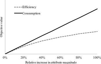
Juxtaposing Figure 2 on top of Figure 1 would lead to some interesting and important predictions on how evaluation mode can have a different impact on people’s preferences and reactions to relative increases (upgrades) given in consumption vs. efficiency measures. In general, Figure 1 shows that the curve of preferences would be (approximately) linear under JE and concave (curvilinear) under SE. Thus, if an upgrade is given in consumption measures, and people are asked to judge it under JE, their subjective value judgments are expected to be linear, which would correspond to the actual objective value gained in this case. Thus, their preferences (WTP) would align with the actual objective value curve, leading them to unbiased preferences. In contrast, if the upgrade is given in consumption measures but people are asked to judge it under SE, their subjective value judgments are expected to be curvilinear (concave, as the SE curve in Figure 1), leading them away from the actual objective value that could be gained (as shown in Figure 2). Thus, their preferences (WTP) would no longer align with actual objective value, showing a systematic under-evaluation of larger upgrades, and this bias is expected to increase as the upgrades increase. Such findings would be consistent with the findings of the studies previously reviewed that focused on JE vs. SE judgments (e.g., Hsee et al., 2005).
However, if the upgrade is given not in consumption but in efficiency measures, then juxtaposing Figure 1 and Figure 2 would yield the opposite pattern. If the upgrade is given in efficiency terms, and people are asked to judge it under JE, then their subjective value judgments are expected to be linear (Figure 1), which would not align with the actual objective value that could be gained (Figure 2). Thus, for efficiency upgrades presented in JE mode, people’s preferences (WTP) are expected to show systematic over-evaluation of larger upgrades, and this bias is expected to increase as the upgrades increase. This pattern is consistent with the findings of the various studies that explored the MPG Illusion or the time-saving bias (e.g., Larrick et al., 2015; Svenson, 2008).
The last implication of juxtaposing Figure 1 and Figure 2 is probably the most interesting and novel one. If the upgrade is given in efficiency, and people are asked to judge it under SE, then their subjective value judgments would follow a concave and curvilinear curve (Figure 1) which would somewhat align with the actual objective value that could be gained (Figure 2). This would mean that their preferences (WTP) would be less biased in most of the cases. Specifically, in the relatively larger upgrades (the right-hand side of the x-axis on Figure 2), where the marginal objective value that could be gained from upgrades is small, people’s diminished sensitivity under SE would actually help them avoid the biases of the ECG (MPG Illusion and time-saving bias) and their preferences (WTP) could be unbiased. However, for the smaller upgrades (the left-hand side of the x-axis on Figure 2), people’s preferences might still be biased, as they may overestimate the gains that could be made there. To summarize, applying the predictions of subjective value judgments from evaluability theory (Hsee & Zahng, 2004) to the objective value functions of the ECG suggests an interaction effect between evaluation mode (JE vs. SE) and the measure (efficiency vs. consumption): WTP for upgrades in consumption would be less biased under JE vs. SE, whereas WTP for upgrades in efficiency would be less biased under SE vs. JE. The latter prediction would mostly occur for relatively large upgrades. Table 1 summarizes the predicted bias in WTP depending on the measure (that determines objective value curve) and the evaluation mode (that determines the subjective value curve).
Table 1: Predicted bias in WTP depending on measure and evaluation modes.
Evaluation Mode and Subjective judgments curve
Under-evaluation of larger upgrades
Over-evaluation of larger upgrades
We examined these hypotheses in two experiments. Study 1 presented participants with four vignettes describing two (a smaller and a larger) upgrades relating to speed or fuel efficiency in either SE or JE modes and participants indicated their WTP for each upgrade (a Supplement details a similar pilot study we conducted with lower statistical power). We predicted that the relative difference in WTP between the smaller vs. larger upgrades would be larger in JE vs. SE. Study 2 expanded these findings to a series of six upgrades, to show that the WTP curve under JE is indeed much more linear than the more concave curve observed under SE. Study 2 also corroborated that when the attribute is given in terms of consumption, WTP becomes less biased in JE than in SE.
Participants. We recruited 1101 participants from Prolific Academic (Mage = 32.8; SDage = 11.7; 50% were female). Participants were pre-screened to include only U.S. residents, aged 18 or above, who speak English as their first language. In order to maximize participants’ attention, and to screen out participants who did not read the instructions carefully, we included an attention-check question asking participants about the topic of the study. In the text preceding the question, participants were instructed to choose the “other” option and write the word “attention” in the adjacent box. Nighty-three participants (8%) failed the attention-check and were omitted from further analyses, so the final sample included 1,008 participants (we increased the pre-registered sample size of 1,000 participants to compensate for the participants failing the attention-check question). All participants received 0.5 GBP for completing the study.
Design, materials, and procedure. The study was presented as a study on consumer preferences. Participants read four scenarios, containing offers of upgrades for two services (Internet service and a fast lane for driving) and two products (a printer and a car). In each scenario, participants were presented with initial values of efficiency or speed and were asked to indicate how much they would be willing to pay for an upgrade to a higher value. Participants were randomly allocated to evaluate both upgrades jointly (JE condition) or separately (SE condition). For example, the Internet speed scenario in the JE condition read:
Sam and Jill are both customers of two large Internet service providers in the U.S. Sam’s provider offers her the option to upgrade her Internet service from 25 Mbps to 50 Mbps. Jill’s provider offers her the option to upgrade her Internet service from 25 Mbps to 100 Mbps. How much, in your opinion, should each of them be willing to pay more for their monthly service after the upgrade? Use the slider below to indicate your opinion about what should be the difference in USD between the current and upgraded plans’ prices.
The four scenarios asked for WTP to: (1) upgrade home Internet speed (from 25 to 50 or 100 Mbps); (2) drive in a fast lane which allows people to increase driving speed (from 30 to 45 or 60 mph); (3) purchase a printer that prints more pages per minute (from 50 to 100 or 150 pages-per-minute); and (4) upgrade a leased car that has a higher fuel efficiency (from 10 to 20 or 30 MPG). Complete wording for all four scenarios is given in Appendix A. Participants indicated their WTP for each scenario using a slider that ranged from 0 to $30, $50, $100, or $200 for the driving speed, the Internet speed, the printer speed the fuel efficiency, respectively.
The order of the four scenarios was randomized within each experimental group. In the separate evaluation conditions, participants were presented with either the small or the large upgrade for each scenario. We also included an additional JE group in which the order of the two upgrades was reversed – the larger upgrade was presented first, followed by the smaller upgrade. However, we did not find any differences between orders so we analyzed these two groups as one JE condition. At the end of the study, participants reported their age, gender and any comments they may have had. The study design and hypotheses were preregistered at https://aspredicted.org/blind.php?x=jw54f3.
As pre-registered, we omitted responses from the JE conditions that indicated a higher estimate for the smaller upgrade relative to the larger upgrade in a certain scenario, and in all groups, we omitted responses that were more than three standard deviations above the mean. Analyzing the results with the omitted responses did not affect the pattern or significance of the results.
Figure 3 shows the means of WTP for each condition, with 95% confidence intervals. As Figure 3 shows, the difference in mean WTP between the small and large upgrades was much larger under JE than it was under SE. For example, when asked for their WTP to upgrade their home Internet speed from 25 to either 50 or 100 Mbps, participants in the JE conditions were willing to pay about twice as much for upgrading their Internet speed from 25 to 100 vs. from 25 to 50 Mbps (M=$22.09 vs. $10.85, respectively). In contrast, participants in the SE mode were willing to add much less (about only 24%) to the cost of the larger upgrade (M=$17.60 vs. $14.24). Interestingly, the larger upgrade (from 25 to 100 Mbps) saves 50% more time than the smaller one (from 25 to 50 Mbps). For the other three scenarios participants in the JE conditions were willing to pay 70%–90% more for the larger upgrade relative to the smaller upgrade, whereas in the SE condition they were willing to add much less for the larger relative to the smaller upgrades (27%, 13%, and 19% for the respective driving, printer, and fuel efficiency scenarios). Importantly, the larger upgrades in these scenarios actually saved 33%–50% more than the smaller ones, which means that judgments were actually more biased in the JE mode than the SE mode. The complete means and SDs for all conditions are given in the Appendix B. In all four scenarios, the interactions between the mode (JE vs. SE) and the size of the upgrade (small vs. large) were statistically significant (p < .001). Thus, Study 1 found that presenting both larger and smaller upgrades jointly led participants to be willing to pay more for larger upgrades compared to smaller ones, whereas participants were less sensitive to the size of the upgrade under SE.
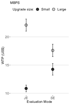
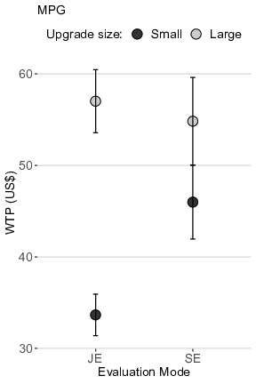
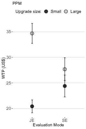
Figure 3: Mean WTP for small or large upgrade in JE vs. SE, in four scenarios of Study 1. Mbps – Internet speed; MPH – driving speed; MPG – fuel efficiency; PPM – printer speed.
The results of Study 1 are consistent with our predictions that judgments of efficiency measures (MPG, Internet, printers’ or driving speed) would follow a linear and magnitude sensitive pattern under JE, but would be less sensitive to magnitude under SE. The same pattern emerged, with little differences, between the scenarios. In all scenarios, the pattern found was that the relatively large difference found under JE was modulated under SE due to the fact that WTPs for the large and small upgrades both got closer: WTP for the small upgrade increased a little and WTP for the large upgrade decreased a little. Thus, all four scenarios revealed a diminished sensitivity to magnitude under SE, vs. a linear relationship between magnitude and WTP under JE, confirming our hypotheses. Moreover, because the actual savings of the larger upgrades follow a curvilinear function of the efficiency upgrade (see Figure 2), participants were actually willing to overpay for these upgrades in the JE conditions, whereas their WTP were less biased in the SE condition.
However, two value points are not enough to infer linear or curvilinear relationships. Thus, in Study 2 we followed Study 1 of Hsee and Zhang (2004) and extended the range of stimuli to include a larger set of upgrades in order to verify that the preference curve under JE would indeed be more linear than the curve under SE. Additionally, we included a consumption measure in Study 2 as a comparison condition to show that the difference in the preferences curve (linear for JE vs. concave for SE) is not the result of a specific speed or efficiency measure but would also manifest using a consumption measure. This condition also serves to fully test our complete model that predicts an interaction effect between mode and measure: JE preferences would be biased for efficiency measures, but SE preferences would be biased for consumption measures.
Participants. We sampled 880 participants (42.6% females, Mage = 34.72, SD = 12.8) from Prolific. We had to screen out 132 (15%) that failed the attention-check question. Participants received 0.2 GBP for completing the study, which was shorter than the previous studies. Participants had to be over 18, from U.S., speaking English as a first language, and did not take part in the previous study.
Design and procedure. Participants were asked to read and respond to a scenario about using a fast lane in order to save time and arrive earlier to a destination. Between-subjects, one scenario presented the fast lane as offering a higher driving speed and the other scenario presented the fast lane as offering a shorter journey time. The speed scenario read:
Imagine you need to complete a journey of 30 miles on an interstate road. The road has two lanes: a regular lane and a fast lane. The fast lane requires paying a fee. The average driving speed on the regular lane is known to be 30 mph, so the journey will take you 60 minutes (one hour) at this speed. The average driving speed on the fast lane is known to be higher. Assuming you need to arrive earlier, how much would you, personally, be willing to pay in order to be able to drive in the fast lane and save time to arrive earlier. Please enter the maximal amount (in US$) you would be willing to pay if you are assured that the average driving speed in the fast lane is the speed given below (compared to 30 mph in the regular lane).
The time scenario read:
Imagine you need to complete a journey of 30 miles on an interstate road. The road has two lanes: a regular lane and a fast lane. The fast lane requires paying a fee. The average driving speed on the regular lane is known to be 30 mph, so the journey will take you 60 minutes (one hour) at this speed. The driving time on the fast lane is known to be shorter. Assuming you need to arrive earlier, how much would you, personally, be willing to pay in order to be able to drive in the fast lane and save time to arrive earlier. Please enter the maximal amount (in US$) you would be willing to pay if you are assured that the total driving time in the fast lane is the time given below (compared to 60 minutes in the regular lane).
Participants were then asked, in the JE condition, to indicate how much they would be willing to pay for six increases of speed (33, 36, 40, 45, 50, and 55 mph, in the speed scenario) or for arriving at earlier times (by 55, 50, 45, 40, 36, and 33 minutes, in the time scenario) using a slider that ranged from 0 to $30. The speed and time values represented the same time savings. Participants in the SE condition were asked about one, randomly chosen, speed or time from these values. All participants then reported their age, gender, and any comments they may have had. The design and hypotheses of Study 2 were preregistered at https://aspredicted.org/blind.php?x=ws9s4i.
As pre-registered, we omitted responses from the JE conditions that indicated a higher estimate for the smaller upgrade relative to the larger upgrade, and in all groups, we omitted responses that were more than three standard deviations above the mean. Analyzing the results with the omitted responses did not affect the pattern or significance of the results. Figure 4 shows the mean WTP for the different speed/time upgrades, in terms of the time saved (from 5 to 27 minutes) between the joint and separate evaluation modes.
As can be seen in Figure 4, in the JE condition, participants’ WTP followed a monotonically increasing pattern, as they were willing to pay marginally more for each speed increase or journey time decrease. In contrast, in the SE condition the means of WTP participants indicated were much less sensitive to the degree of speed increased or amount of journey time reduced.
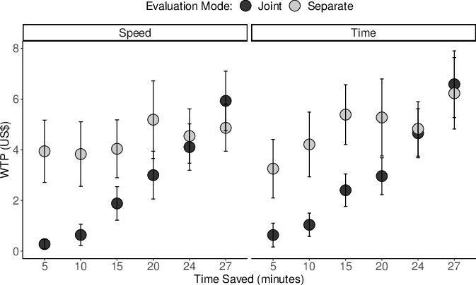
Figure 4: Mean WTP (US$) for upgrading driving speed or journey time, in six levels of time saved, in joint vs. separate evaluation.
To analyze these patterns statistically, we performed separate tests for each condition, because observations were independent in the SE condition and repeated in the JE condition. First, we conducted a repeated measures analysis on the WTP in the JE condition, with amount of time saved as the within-subjects factor, and the measure of the scenario (speed or time) as a between-subjects factor. We found a statistically significant effect for the time saved (F(5,520) = 173.44, p < .001), but no main effect for the measure (F(5,104) = 0.29, p = 0.92), and no significant interaction of the time and measure (F(1,104) = 0.92, p = 0.34). For the SE condition, in which WTPs were independent between levels of time saved, we conducted an ANOVA with time saved and measure as between-subjects factors. We found a significant effect for time saved (F(5,598) = 2.78, p = 0.02), but no significant effect for the measure (F(1,598) = 1.7, p = 0.19) or the interaction (F(5,598) = 0.81, p = 0.54). However, additional tests of the SE condition showed that the time saved had no significant effect in the speed measure scenario (F(5,301) = 0.85, p = 0.52). Also, although in the time measure scenario, the effect of time saved was significant (F(5,297) = 2.69, p = 0.02), subsequent post-hoc tests showed the difference was only significant between the WTP for saving 5 minutes vs. 27 minutes (i.e., the two extreme ends of the scale).
These results show that participants’ sensitivity to the offered upgrades in speed (or time) was evident only when the upgrades were presented jointly, but this sensitivity diminished when the same upgrades were evaluated separately. Apparently, when given several upgrades to be judged jointly, people are willing to pay more for a larger upgrade (that offers a larger benefit) but not so when the same upgrades are evaluated each on its own. In the latter case, it appears that people apply a kind of categorical heuristic by which they only decide whether they are or are not willing to pay in order to obtain the benefit of the offered upgrade, and base their decision only on the offer of the upgrade, disregarding the size of the offered upgrade.
The findings of both studies showed the interaction between evaluation mode (JE vs. SE) and judgment of upgrade savings, when presented using efficiency vs. consumption measures. Study 1 showed that under JE mode, participants’ WTP was higher for larger vs. smaller efficiency upgrades, whereas under SE mode participants showed a diminished sensitivity to the magnitude of the upgrade. As the actual savings are a curvilinear function of the upgrades, these findings confirm our hypothesis that given efficiency upgrades, judgments are more biased under JE relative to SE mode. Study 2 showed that participants’ WTP is linearly related to the upgrades under JE, whereas their WTP is a curvilinear function of the upgrades under SE, whether the upgrades are presented by efficiency or consumption measures. These findings confirm our hypotheses about the interaction between evaluation mode (JE vs. SE) and efficiency vs. consumption measures: For consumption measures, the subjective value under JE is less biased than under SE, whereas for efficiency measures the opposite is true: judgments under SE are less biased than under JE.
For upgrades presented with consumption measures, our findings are consistent with the previous work of Hsee and colleagues (Hsee, 1998; Hsee & Zhang, 2004; Hsee et al., 2005), demonstrating that people are more magnitude sensitive under JE than under SE. These findings were explained by the evaluability theory, arguing that people evaluate options using attributes that are easier to evaluate, and less by attributes that are harder to evaluate, even when the latter might be more important, such as the amount of a product. In such cases, under JE mode, people would provide evaluations that are less biased, as the more important attribute, such as different amounts of a product, might be evaluated more easily. Similarly, given upgrades using consumption measures, the value of the upgrade would be more difficult to evaluate under SE, and more easy to evaluate under JE. Referring back to Figure 2, the actual value of the savings represented by the solid line, would align with the linear function representing the subjective value under JE in Figure 1, and not align with the concave curve representing the biased subjective value under SE. Thus, with respect to consumption measures, our findings regarding judgments of upgrades are consistent with previous findings comparing JE and SE with respect to various amounts/magnitudes of products (Hsee, 1998; Hsee & Zhang, 2004; Hsee et al., 2005), demonstrating the unbiased judgments under JE vs. the biased ones under SE.
However, presenting upgrades using efficiency measures, rather than consumption measures, results in actual savings that follow a curvilinear function of the magnitude of the upgrade (the dashed line in Figure 2). The findings of this paper show that when presented with two (or more) efficiency upgrades under JE mode, participants provide judgments that are linearly related to the magnitude of the upgrade often resulting in incorrect and biased judgments. These findings are consistent with previous demonstrations of what we have termed as the Efficiency-Consumption Gap (ECG): People underestimate the impact of increases from relatively lower efficiency values and overestimate the impact of increases from relatively higher values (the MPG Illusion, Larrick & Soll, 2008; the time-saving bias, De Langhe & Puntoni, 2016; Peer & Gamliel, 2013; Svenson, 2008). Critically, however, these biased judgments of efficiency upgrades under JE seem to be corrected under SE: Individuals’ insensitivity to the magnitude of the upgrade under SE, represented by the curvilinear dashed line in Figure 1, align with the actual savings to efficiency upgrades (the curvilinear dashed line in Figure 2). This alignment reflects a unique combination in which “two wrongs can make a right”: People’s insensitivity to magnitude under SE (“one wrong”) matches the non-intuitive curvilinear function relating actual savings to efficiency upgrades (“second wrong”), establishing the unique “right” outcome, namely, unbiased evaluations of efficiency upgrades under SE. In other words, SE can de-bias some of the errors people make when judging efficiency upgrades.
However, this finding probably does not mean that when given efficiency upgrades under SE people suddenly realize or understand that the relationship between efficiency and consumption is curvilinear. More likely is that the bias of the ECG persists and is coupled by the bias of the SE mode, which, in our particular case, negate each other and lead people to behave as if they are making rational judgments. This effect is analogous to findings in other domains that have shown that sometimes one bias can be exploited and used to counter another bias and lead people to better judgments and decisions. For example, people are known to be present biased, especially when it comes to enrolling in pension plans, and thus save too little (e.g., Soman et al., 2005). At the same time, people are also very sensitive to default choices, opting out of them less than they would opt in (e.g., Johnson & Goldstein, 2013). The Save More Tomorrow program (Thaler & Benartzi, 2004) intentionally exploits the default bias to counter present bias such that employees are automatically enrolled in a pension plan and this default enrollment counters their present bias. As in their case, also in ours one bias (diminished sensitivity under SE) is used to counter another bias (the ECG). However, just like the Save More Tomorrow program does not make people less present biased in mind, only in their behavior, the same probably occurs in our case: people do not become aware of the non-linear relationship of efficiency and consumption under SE. They simply behave as if they do.
These findings have both theoretical and empirical implications. Theoretically, we propose a model that compares two functions – one relating subjective value with mode of evaluation (JE or SE), and the other relating actual savings following an upgrade that is presented in either consumption or efficiency measures. This comparison enables us to present each type of evaluation mode as unbiased given one type of measure, and biased given the other type of measure. Previous research on the ECG did not explicitly consider the role of the mode of evaluation, and we show that it can have considerable implications for our understanding of people’s judgements, and probably their actual choices (although that would warrant more research). Additionally, previous research on the ECG typically used pairs of upgrades (e.g., 10 to 15 MPG vs. 30 to 35 MPG) to show people’s biases. However, in real life situations, individuals do not typically consider pairs of upgrades but they have one initial starting point (the current efficiency of their product, for example) and are contemplating one, two or more levels of upgrades. The fact that the same biases of the ECG were also found in our studies, which used the same (and not different) initial points, corroborates the findings of previous studies and adds an important element of ecological validity to their conclusions.
Our findings can also be extended to situations in which people consider downgrading the quality of their product. For example, a consumer may wish to switch to a lower Internet speed plan, should she wish to save some on her budget. In these cases, the ECG would state that most consumers would overestimate the loss incurred when downgrading from high values, and underestimate the loss incurred when downgrading from low values (e.g., Svenson & Borg, 2020). In these cases, if the consumer would judge several downgrade options of an efficiency measure (e.g., Mbps), she would be less biased if that is done under SE vs. JE. Conversely, she would be more biased if she were to consider the same downgrade options in consumption measures (e.g., seconds to download 100 Mb) under SE vs. JE. This raises an interesting question: how, then, would consumers judge between an option to upgrade (pay more to gain speed) vs. an option to downgrade (lose speed to gain money), when both are compared to the consumer’s current initial status or to a benchmark starting offer? Future research could empirically test this question and explore whether the interaction between evaluation mode and measure operates differently when considering only upgrades, only downgrades, or both.
Another interesting theoretical implication would involve the relative size of the upgrade compared to the initial point. When one juxtaposes Figures 2 on 1, as we suggested earlier, it is apparent that, for relatively large upgrades, the diminishing sensitivity curve of the SE judgments closely aligns with the diminishing utility curve of the efficiency measure. However, for relatively smaller upgrades, it is not clearly apparent whether, and to what extent, would SE judgments be less biased than JE judgments. Future research could manipulate the values of efficiency upgrades in a range that starts from very small increases (e.g., 5%) to very large ones (e.g., 500%), in order to demonstrate the match of WTP in SE mode, and the mismatch of WTP in JE mode. We would predict that the curvilinear subjective value function of the SE mode and the linear function of the JE mode would reveal willingness to overpay in the SE mode for relatively small upgrades, and willingness to overpay in the JE mode for relatively larger upgrades. However, the extent of these differences may rely on other factors such as the context and the stakes involved.
We demonstrated that joint evaluations of smaller and larger upgrades lead people to be willing to overpay for larger efficiency upgrades. Consumers’ awareness of their biased WTP in these contexts might assist them in reducing their susceptibility to this bias. Overpaying for larger efficiency upgrades of products and services not only harms the consumer in the short-term, but may also decrease innovation and adversely affect market efficiency in the long-term (De Langhe & Puntoni, 2016). Thus, policymakers and regulators might benefit from understanding how evaluation modes affect decision-making in the context of the ECG, and use that knowledge to design policies that ensure that consumers are afforded the most appropriate, and less biased, mode of evaluation when making judgments and decisions that relate to efficiency and consumption.
De Langhe, B., & Puntoni, S. (2016). Productivity metrics and consumers’ misunderstanding of time savings. Journal of Marketing Research, 53(3), 396–406.
De Langhe, B., Puntoni, S., & Larrick, R. P. (2017). Linear thinking in a nonlinear world. Harvard Business Review, 95(3), 130–139.
Eriksson, G., Svenson, O., & Eriksson, L. (2013). The time-saving bias: Judgements, cognition and perception. Judgment and Decision Making, 8(4), 492–497.
Hsee, C. K. (1996). The evaluability hypothesis: An explanation for preference reversals between joint and separate evaluations of alternatives. Organizational Behavior and Human Decision Processes, 67, 247–257.
Hsee, C. K. (1998). Less is better: When low-value options are valued more highly than high-value options. Journal of Behavioral Decision Making, 11, 107–121.
Hsee, C. K. (2000). Attribute evaluability and its implications for joint-separate evaluation reversals and beyond. In D. Kahneman & A. Tversky (Eds.), Choices, Values, and Frames (pp. 543-563). New York: Cambridge University Press.
Hsee, C. K., & Rottenstreich, Y. (2004). Music, pandas, and muggers: on the affective psychology of value. Journal of Experimental Psychology: General, 133(1), 23.
Hsee, C. K., Rottenstreich, Y., & Xiao, Z. (2005). When is more better? On the relationship between magnitude and subjective value. Current Directions in Psychological Science, 14(5), 234–237.
Hsee, C. K., & Zhang, J. (2004). Distinction bias: Misprediction and mischoice due to joint evaluation. Journal of Personality and Social Psychology, 86(5), 680–695.
Hsee, C. K., & Zhang, J. (2010). General evaluability theory. Perspectives on Psychological Science, 5(4), 343-355.
Johnson, E. J., & Goldstein, D. G. (2013). Decisions by default. In E. Shafir (Ed.), The behavioral foundations of public policy (p. 417–427). Princeton University Press.
Kogut, T., & Ritov, I. (2005). The singularity effect of identified victims in separate and joint evaluations. Organizational Behavior and Human Decision Processes, 97(2), 106–116.
Larrick, R. P., & Soll, J. B. (2008). The MPG illusion. Science, 320(5883), 1593–4.
Larrick, R. P., Soll, J. B., & Keeney, R.L. (2015). Designing better energy metrics for consumers. Behavioral Science & Policy, 1(1), 63-75.
List, J. A. (2002). Preference reversals of a different kind: The “More is less” Phenomenon. American Economic Review, 92(5), 1636–1643.
Peer, E. (2010). Exploring the time-saving bias: How drivers misestimate time saved when increasing speed. Judgment and Decision Making, 5(7), 477.
Peer, E. (2011). The time-saving bias, speed choices and driving behavior. Transportation Research Part F: Traffic Psychology and Behaviour, 14(6), 543–554.
Peer, E., & Gamliel, E. (2012). Estimating time savings: The use of the proportion and percentage heuristics and the role of need for cognition. Acta Psychologica, 141(3), 352–359.
Peer, E., & Gamliel, E. (2013). Pace yourself: Improving time-saving judgments when increasing activity speed. Judgment and Decision Making, 8(2), 106–115.
Peer, E., & Solomon, L. (2012). Professionally biased: misestimations of driving speed, journey time and time-savings among taxi and car drivers. Judgment and Decision Making, 7(2), 165.
Small, D. A., & Loewenstein, G. (2003). Helping a victim or helping the victim: Altruism and identifiability. Journal of Risk and Uncertainty, 26(1), 5–16.
Soman, D., Ainslie, G., Frederick, S., Li, X., Lynch, J., Moreau, P., Mitchell, A., Read, D., Sawyer, A., Trope, T., & Wertenbroch, K. (2005). The psychology of intertemporal discounting: Why are distant events valued differently from proximal ones?. Marketing Letters, 16(3-4), 347–360.
Svenson, O. (1970). A functional measurement approach to intuitive estimation as exemplified by estimated time savings. Journal of Experimental Psychology, 86(2), 204.
Svenson, O. (1973). Change of mean speed in order to obtain a prescribed increase or decrease in travel time. Ergonomics, 16(6), 777-782.
Svenson, O. (1976). Experience of mean speed related to speeds over parts of a trip. Ergonomics, 19(1), 11–20.
Svenson, O. (2008). Decisions among time saving options: When intuition is strong and wrong. Acta Psychologica, 127, 501–509.
Svenson, O. (2011). Biased decisions concerning productivity increase options. Journal of Economic Psychology, 32(3), 440–445.
Svenson, O., & Borg, A. (2020). On the human inability to process inverse variables in intuitive judgments: different cognitive processes leading to the time loss bias. Journal of Cognitive Psychology, 32(3), 344-355.
Thaler, R. H., & Benartzi, S. (2004). Save more tomorrow™: Using behavioral economics to increase employee saving. Journal of political Economy, 112(S1), S164-S187.
Internet speed: Sam and Jill are both customers of two large Internet service providers in the U.S. Sam’s provider offers her the option to upgrade her Internet service from 25 Mbps to 50 Mbps. Jill’s provider offers her the option to upgrade her Internet service from 25 Mbps to 100 Mbps. How much, in your opinion, should each of them be willing to pay more for their monthly service after the upgrade? Use the slider below to indicate your opinion about what should be the difference in USD between the current and upgraded plans’ prices.
Fuel efficiency: Mark and George are two unrelated persons who have recently received a leased car from their workplace, on which they pay a monthly payment (which includes all expenses except for fuel costs). They both got offers to upgrade their car for an increase in their monthly payment. The cars are identical in all aspects except for their fuel efficiency: Mark’s current car gets, on average, 10 Miles Per Gallon (MPG), and was offered to upgrade to a car that gets 20 MPG on average. George’s current car gets, on average, 10 Miles Per Gallon (MPG), and was offered to upgrade to a car that gets 30 MPG on average. How much, in your opinion, should each of them be willing to pay more in their monthly payment for the car with the better fuel efficiency (higher MPG)? Use the slider below to indicate your opinion about what should be the difference in USD between the monthly payments in each case.
Printers speed: Peter and Patrick are two unrelated persons who ordered a new printer online for their home. After check-out, they receive an offer to upgrade their chosen printer to a faster one. The printers are identical in all aspects except for their printing speed. Peter ordered a printer that prints 50 Pages Per Minute (PPM), and was offered to upgrade to a printer that prints 100 PPM. Patrick ordered a printer that prints 50 Pages Per Minute (PPM), and was offered to upgrade to a printer that prints 150 PPM. How much, in your opinion, should each of them be willing to pay more for the offered printer that is faster (has a higher PPM)? Use the slider below to indicate your opinion about what should be the difference in USD between the prices of the printers in each case.
Driving speed: Keren and Helen are two unrelated persons. They are each at different locations, and each need to drive to a destination that is 50 miles away from their current location. They both want to get to their destination quickly, and each can choose to use the “fast lane” that offers higher average driving speed, at the same distance, but requires a fee. Keren’s choices are to either take the regular lane, in which the average driving speed is 30 Mph, or a fast lane in which the average driving speed is 45 Mph. Helen’s choices are to either take the regular lane, in which the average driving speed is 30 Mph, or a fast lane in which the average driving speed is 60 Mph. How much, in your opinion, should each of them be willing to pay to use the fast lane for the journey of 50 miles? Use the slider below to indicate your opinion about what should be the price in USD for using the fast lane in each case.
Appendix B. Means of WTP (and SDs) for the smaller and larger upgrades in joint vs. separate evaluations for the scenarios (Study 1).
Internet speed Fuel efficiency Printer speed Driving speed Condition Upgrade N M SD N M SD N M SD N M SD SE Small 251 14.24 8.29 251 45.99 32.48 250 24.40 17.17 249 5.80 4.38 Large 250 17.60 8.82 251 54.83 38.48 250 27.67 18.04 251 7.34 5.51 JE Small 480 10.85 6.59 466 33.66 24.89 474 20.42 13.94 477 4.72 4.19 Large 22.09 11.96 57.02 37.85 34.68 21.60 9.04 6.67 JE-Asc. Small 242 10.96 6.80 237 35.06 25.84 240 20.36 13.55 242 4.47 3.95 Large 22.03 12.17 57.42 40.47 34.04 21.62 8.49 6.47 JE-Des. Small 238 10.74 6.39 229 32.20 23.84 234 20.49 14.35 235 4.98 5.44 Large 22.14 11.77 56.61 35.07 35.34 21.61 4.42 6.84
Copyright: © 2021. The authors license this article under the terms of the Creative Commons Attribution 3.0 License.
This document was translated from LATEX by HEVEA.
