Judgment and Decision Making, Vol. 15, No. 6, November, 2020, pp. 1044-1051
Reanalysis of Butler and Pogrebna (2018) using true and error model
Michael H. Birnbaum*
|
Butler and Pogrebna (2018) devised triples of three-branch gambles theorized to violate transitivity of preference according to a most probable winner model. According to this model, a person chooses the option that has the higher probability to yield a better outcome than the other alternative. They tested 11 triples with 100 participants and found cases that appeared to violate weak stochastic transitivity and the triangle inequality. But tests of weak stochastic transitivity and the triangle inequality do not provide a proper method to compare transitive and intransitive models that allow mixtures of preference patterns and random errors. Those older methods can yield false conclusions regarding transitivity, for example, if different participants have different true preferences or if different choice problems have different rates of error. This paper reanalyzes their data using a true and error (TE) model, which does not require these unrealistic assumptions, and which provides estimates of the incidence of transitive and intransitive behavior in a mixture. Reanalysis indicated that 3 of the 11 triples showed convincing evidence of violations of transitivity in the opposite direction of the predictions of the most probable winner model. Further, these and other triples showed other significant violations of the most probable winner model. Despite some violations of the true and error model, the data of Butler and Pogrebna appear to contradict not only transitive utility models but they also refute the most probable winner model as a descriptive theory of choice behavior.
Keywords: error theory, risky decision making, transitivity, regret theory
1 Introduction
If preferences are transitive, then if X is preferred to Y and Y is preferred to Z, then X is preferred to Z. Many people consider transitivity to be both rational and also descriptive of risky decision making. But there are some who argue that transitivity is neither rational nor descriptive (e.g., Fishburn, 1991; Butler & Blavatskyy, 2020; McNemara, et al., 2014).
Butler and Pogrebna (2018) theorized that if a person follows a binary decision rule of choosing the alternative that has a higher probability of yielding a better outcome, then that person would show systematic violations of transitivity of preference in specially constructed choice problems. This decision strategy is known as the most probable winner (MPW) model, and is sometimes known as majority rule.
For example, consider gambles with three equally likely consequences, X = (x1, x2, x3), denoting equal chances to win $x1, $x2, or $x3. Suppose X = (15, 15, 3), Y = (10, 10, 10), and Z = (27, 5, 5). If the prizes received under X, Y, Z are statistically independent, then the probability that X gives a higher outcome than Y is 2/3; the probability that Y gives a higher outcome than Z is 2/3; and the probability that Z gives a higher outcome than X is 5/9. So, if people choose by MPW, their choices would be intransitive with this triple.
The MPW model is an extreme special case of the additive difference models, a class of models investigated by Birnbaum and Diecidue (2015) that also includes regret theory (Loomes & Sugden, 1982) as a special case. Regret theory implies the opposite pattern of intransitivity (See Appendix) from that of MPW. Birnbaum and Diecidue (2015) found very few individuals whose data showed either type of intransitive response patterns; they also found that the data showed systematic violations of restricted branch independence, a property implied by the additive difference models.
Butler and Pogrebna (2018) conjectured that intransitive behavior might be observed when there are no more than two distinct outcome values in each gamble, and when riskier gambles have slightly higher expected values (EV) than safer ones. In this example, the most risky gamble, Z has an EV of 12.33, medium risky gamble, X, has an EV = 11, and the safest gamble, Y, has the lowest EV, 10. There were a total of 11 triples with similar values constructed from this recipe.
| Table 1: Crosstabulation. Frequencies of response patterns in first repetition (rows) and second repetition (columns) of Triple 4 in Butler and Pogrebna (2018). This triple showed the higest incidence of intransitive behavior. |
| | 121 | 123 | 131 | 133 | 221 | 223 | 231 | 233 |
121 | 2 | 3 | 0 | 0 | 0 | 1 | 4 | 1 |
123 | 0 | 0 | 0 | 0 | 0 | 0 | 0 | 0 |
131 | 0 | 0 | 2 | 0 | 0 | 0 | 4 | 0 |
133 | 1 | 0 | 1 | 1 | 0 | 0 | 2 | 1 |
221 | 0 | 3 | 0 | 0 | 1 | 4 | 1 | 0 |
223 | 0 | 2 | 1 | 1 | 1 | 0 | 0 | 0 |
231 | 5 | 8 | 1 | 1 | 5 | 12 | 26 | 1 |
233 | 0 | 2 | 0 | 0 | 0 | 0 | 2 | 0 |
| Total n = 100. The most probable winner model implies the intransitive pattern 123; the opposite pattern, 231, is also intransitive. |
For each triple of gambles, X, Y, and Z, there are three binary choice problems, XY, YZ, and ZX. In XY the response can be coded as 1 if the X is chosen, and 2 if Y; in YZ, code 2 or 3 if Y or Z was chosen; in ZX, code 1 or 3 if X or Z was preferred, respectively. There are 8 possible preference patterns: 121, 123, 131, 133, 221, 223, 231, or 233, two of which are intransitive, 123 and 231. For these X, Y, and Z, the MPW model implies 123. Other theories are discussed in the Appendix.
Butler and Pogrebna used these three gambles (in pounds rather than dollars) and 10 other, similar triples of gambles; they obtained three binary choices in each triple, which were presented twice to each of 100 participants. In between the two repetitions of the binary choice task, participants were asked to rank the three gambles in each triple, which forces a transitive order. Because the intervening task of ranking may have affected preferences, I use the term "repetitions" rather than "replications" for the two presentations of the binary choices.1
1.1 Problems with Previous Analyses
In previous research, there has been a long standing problem of how to test transitivity when there might be random errors in the data, when the error rates in different choice problems might be unequal, and when data might include a mixture of true preference patterns, either because different people have different true preferences or because the same person may change preferences over time. It turns out that methods of analysis used in the past cannot be relied upon in such cases to properly evaluate the issue of transitivity; those methods can easily fail to correctly diagnose whether data arose from a transitive or intransitive true preference structure.
Sopher and Giglioti (1993) noted that if different choice problems have different rates of error, then tests of transitivity based on inequality of response patterns (once considered evidence of intransitivity) might easily signal "intransitivity" when the data are actually perfectly transitive. Birnbaum and Schmidt (2008) gave clear examples to illustrate that one cannot properly address the issue of transitivity without measuring error rates in the choice problems used to measure preferences and test transitivity. They noted that with proper experimental designs, the true and error model can be used to estimate error rates and can resolve this problem.
Regenwetter, Dana, and Davis-Stober (2011) developed statistical tests of weak stochastic transitivity and the triangle inequality based on the assumptions that choice responses satisfy independence and identical distribution (iid). However, Birnbaum (2012), Birnbaum and Bahra (2012) and others have reported evidence that iid is systematically violated by empirical data, so these new statistical tests are dubious.
But there are even more fundamental problems with testing these properties of binary choice probabilities (than issues with the statistical assumptions): Tests of the triangle inequality and weak stochastic transitivity cannot properly diagnose the issue of transitivity when the data might arise from a mixture of true preferences. The triangle inequality and weak stochastic transitivity can both be perfectly satisfied in cases where the vast majority of participants systematically violated transitivity, and weak stochastic transitivity can be significantly violated in a group of data in which every individual was perfectly transitive but different participants had different true preferences.2
Furthermore, statistical tests (of properties like weak stochastic transitivity) give only a "reject" or "retain" answer. They do not provide estimates of the incidences of different transitive and intransitive response patterns, which one needs in order to evaluate models of decision making. Birnbaum and Wan (2020) simulated data from transitive or intransitive processes and illustrated that those older methods of analysis simply cannot correctly identify whether a transitive or intransitive model had been used to create the data. They also showed that the true and error model correctly identified whether a transitive or intransitive model had been used to generate the data in these cases where the older methods fail.
Because the data analyses presented in Butler and Pogrebna (2018) were based on these older methods, a skeptic could remain unconvinced that their data actually contained any real evidence against transitivity, once errors and differences in true preferences are allowed. Fortunately, because their study included two presentations of each choice problem, it is possible to apply the true and error (TE) model to reanalyze their data in order to estimate error rates and the incidence of intransitive and transitive behavior (Birnbaum, 2013; Birnbaum, Navarro-Martinez, Ungemach, Stewart, & Quispe-Torreblanca, 2016; Birnbaum & Wan, 2020)
1.2 True and Error Fitting Model
The numbers of participants who showed each of the response patterns on first and second repetitions for Triple #4 of Butler and Pogrebna (2018) are shown in Table 1. This triple appeared to have the strongest evidence of intransitivity. Rows represent the response pattern on the first repetition of the binary choice problems, and the columns show the response pattern on the second repetition. There were 26 people out of 100 participants who showed intransitive cycle (231) on both repetitions. There were 33 others who showed the 231 response pattern on the first repetition and switched to other patterns on the second repetition, including 12 who switched to 223 and 8 who reversed all three preferences to 123. However, not even one participant responded on both occasions with this intransitive pattern (123) implied by the MPW model. Although Table 1 did not appear in the published version of Butler and Pogrebna (2018), this table and those for the other triples are included in the journal’s Online supplement to their paper.
The TE model can be fit to Table 1 and the corresponding tables for the other triples.
There are two sets of parameters in a group TE model: the probabilities of making errors in each of the three choice problems, denoted e1, e2, and e3; and the probabilities of the 8 possible true preference patterns, p121, p123, p131, p133, p221, p223, p231, and p233, which represent the distribution in the mixture of true preference patterns among the individuals. According to the TE fitting model used here, the predicted frequency that people will show the response pattern 123 (implied by MPW) on two replications (of three choice problems) is given as follows:
|
| | P123,123 = n[p121(1−e1)2(1−e2)2(e3)2 | | | | | | | | | | |
|
+ p123(1−e1)2(1−e2)2(1−e3)2 | | | | | | | | | | |
|
+ p131(1−e1)2(e2)2(e3)2 | | | | | | | | | | |
|
+ p133(1−e1)2(e2)2(1−e3)2 | | | | | | | | | | |
|
+ p221(e1)2(1−e2)2(e3)2 | | | | | | | | | | |
|
+ p223(e1)2(1−e2)2(1−e3)2 | | | | | | | | | | |
|
+ p231(e1)2(e2)2(e3)2 | | | | | | | | | | |
|
+ p233(e1)2(e2)2(1−e3)2]
| | | | | | | | | | |
|
where P123,123 is the predicted frequency (count) of the 123 response pattern in both repetitions of the task (i.e., six separate binary choice responses on different trials), and n is the number of participants. Note that if a person has the true preference pattern of 123, then she or he would have to make no errors on six separate choice problems to exhibit this response pattern, and if the true pattern were 121, then she or he made an error on the third choice problem twice. This expression is one of the 64 equations for the predicted frequencies of the 64 possible response patterns, as in Table 1. The "predicted" (or "fitted") frequencies corresponding to the data in Table 1 are simply n times the theoretical probabilities, using parameter estimates best-fit to the data.
| Table 2: Parameter estimates in TE fitting models with 95% confidence intervals. |
Triple | p121 | p123 | p131 | p133 | p221 | p223 | p231 | p233 | e1 | e2 | e3 |
1 | 00 (00−11) | 03 (00−10) | 00 (00−08) | 05 (00−18) | 44 (30−58) | 08 (00−16) | 20 (02−31) | 20 (06−32) | 28 (13−35) | 16 (00−32) | 00 (00−22) |
2 | 33 (00−67) | 21 (00−34) | 25 (00−56) | 00 (00−16) | 00 (00−00) | 21 (00−33) | 00 (00−13) | 00 (00−34) | 20 (00−29) | 41 (19−46) | 11 (00−36) |
3 | 15 (00−26) | 20 (06−32) | 00 (00−01) | 00 (00−13) | 37 (21−56) | 10 (00−21) | 09 (00−26) | 09 (00−23) | 13 (00−31) | 28 (11−36) | 08 (00−30) |
4 | 04 (00−12) | 37 (00−52) | 00 (00−02) | 01 (00−06) | 00 (00−00) | 07 (00−39) | 51 (40−62) | 00 (00−00) | 26 (17−33) | 10 (00−20) | 12 (03−21) |
5 | 06 (00−18) | 04 (00−11) | 00 (00−07) | 19 (07−29) | 46 (32−60) | 03 (00−13) | 21 (02−32) | 01 (00−11) | 23 (02−33) | 09 (00−30) | 14 (00−27) |
6 | 07 (00−20) | 01 (00−08) | 00 (00−00) | 09 (00−23) | 52 (33−67) | 02 (00−11) | 17 (06−26) | 13 (01−25) | 26 (13−35) | 00 (00−21) | 22 (02−31) |
7 | 00 (00−02) | 00 (00−00) | 18 (00−45) | 19 (00−39) | 18 (00−33) | 11 (00−22) | 34 (19−52) | 00 (00−12) | 20 (01−33) | 12 (00−28) | 27 (04−40) |
8 | 09 (00−20) | 08 (01−16) | 04 (00−11) | 11 (04−21) | 57 (45−69) | 02 (00−08) | 09 (00−17) | 00 (00−00) | 14 (00−28) | 06 (00−21) | 10 (00−23) |
9 | 17 (05−25) | 00 (00−05) | 00 (00−08) | 02 (00−08) | 81 (66−89) | 01 (00−12) | 00 (00−00) | 00 (00−07) | 05 (00−17) | 06 (00−12) | 24 (12−31) |
10 | 02 (00−07) | 00 (00−00) | 12 (00−29) | 10 (00−23) | 13 (00−28) | 07 (00−17) | 38 (24−59) | 18 (00−40) | 10 (00−29) | 11 (00−26) | 24 (00−41) |
11 | 00 (00−20) | 25 (00−41) | 14 (00−29) | 00 (00−15) | 28 (00−49) | 01 (00−61) | 00 (00−33) | 33 (00−52) | 20 (00−50) | 29 (21−50) | 30 (18−47) |
| The patterns 123 and 231 are intransitive. Values are expressed as percentages, so 01 indicates 0.01. Numbers in parentheses show 95% bootstrapped confidence intervals. The most probable winner model allows only the 123 pattern in all triples except #5, 8, and 9; in Triple 8, it implies only 121, and it allows either 121 or 123 in #5 and 9. |
Birnbaum’s (2013) Excel spreadsheet, TE8x8_fit.xlsx, [available from the journal’s website supplement to Birnbaum and Wan (2020)] can be used to select parameters to minimize either χ2 or G indices of fit. Minimizing G is equivalent to a maximum likelihood solution. The index G, sometimes denoted G2, is defined as follows:
|
G = 2∑∑Oijln(Oij/Pij)
(1) |
where the summation is over the 64 cells (8 rows by 8 columns), Oij is the observed frequency in the cell (as in Table 1), Pij is the "predicted", or "fitted" frequency. The indices, i and j, represent the 8 response patterns for the rows and columns of tables (as in Table 1), respectively; i.e., i= 1, 2, 3, …, 8 correspond to 121, 123, 131, …, 233, respectively. The χ2, is similar:
|
χ2 = ∑∑(Oij−Pij)2/Pij
(2) |
These indices usually take on similar values, and both are asymptotically Chi-Square distributed.
There are 64 data values in the 8 by 8 tables, which sum to the number of participants, and thus have 63 degrees of freedom (df). The 11 parameters to be estimated use 10 degrees of freedom because the eight probabilities of true preference patterns sum to 1, so the Chi-Squares have 53 df.
The transitive model is a special case of the TE model in which p123 and p231 are both fixed to zero. One can therefore test transitivity by computing the difference between the fits of the TE model and the transitive special case, which is also Chi-Squared distributed with 2 df.
A program in R (Birnbaum, et al., 2016), TE8x2_fit.R, is available from this journal’s website supplement to Birnbaum and Wan (2020). This program can be used to analyze the TE model when sample sizes are relatively small. This program is applied to an 8 by 2 simplification of Table 1, which partitions the data into the 8 diagonal entries and the 8 column sums minus the diagonal entries). It uses Monte Carlo simulations to estimate distributions of the test statistic and it employs bootstrapping to estimate sampling distributions of parameter estimates.3
The TE fitting model allows that different participants may have different true preference patterns, but it assumes that each person maintains the same true preferences in both replications, and it allows that a person might make different responses on two replications due to random errors. The errors are assumed to be mutually independent. The assumption that errors are mutually independent does not imply that responses are independent, except in special cases such as when all persons have the same true preferences (Birnbaum, 2013).
2 Results
Table 2 shows estimated parameters of the TE fitting model applied to the data of Butler and Pogrebna (2018). To save space, numbers are presented as percentages (e.g., 04 indicates 0.04). The ranges in parentheses represent bootstrapped 95% confidence intervals, based on 10,000 bootstrapped samples.
Three of 11 triples (#4, 7, and 10) have convincing evidence of the 231 intransitive pattern. In these three triples, 26, 12, and 17 people (out of 100) showed this same pattern on both repetitions, and the TE fitting model gave estimated probabilities of p231 = 0.51, 0.34, and 0.38, respectively. The lower bounds of the confidence intervals are 0.40, 0.19, and 0.24, respectively, giving confidence that the incidence of intransitive behavior is more than trivial in these three triples.
In Triple # 4, X = (15, 15, 3), Y = (10, 10, 10), and Z = (27, 5, 5); in Triple #7, X = (9, 9, 3), Y = (6, 6, 6), Z = (16, 4, 4); in Triple #10, X = (14, 14, 2), Y = (8, 8, 8), Z = (21, 6, 6). According to the MPW model, these three triples should have shown only the 123 true preference pattern. Instead, there is systematic evidence of the opposite pattern of intransitive behavior and of transitive patterns not allowed by MPW.4
There is also evidence of small incidence of the 231 pattern in Triples 1, 5, and 6. Averaged over all triples, the estimated incidence of the 231 cycle was 0.18, meaning that on average, 18% of participants appear to manifest this intransitive true preference pattern with the triples generated with this recipe. Although 18% does not represent the majority of participants, this rate of intransitive behavior is higher than that reported in previous studies with similar choice tasks (Birnbaum & Diecidue, 2015).
Evidence of the intransitive pattern implied by the MPW model, however, appears to be weaker and less convincing than evidence of the opposite. The best case for the 123 pattern implied by MPW is in Triple #3, where only 7 of 100 participants repeated the 123 pattern in both repetitions; the lower limit of the confidence interval for pattern 123 is only 0.06.
The argument that the 123 pattern may result from use of the MPW is thus weak and is made even less compelling because MPW implies that these same people should have only the 123 pattern, not only for Triple # 3 but also for all other triples in the study except #5, 8, and 9, including Triples # 4, #7, and #10, where no one repeated the 123 pattern. Using the TE model, one can reject the hypothesis that the incidence of pattern 123 exceeds 0.05 in Triples #7 and #10, G = 51.51 and 8.85, p < 0.01.
| Table 3: Indices of fit of TE model, tests of significance of the 123 pattern, and tests of of transitivity (both 123 and 231) l |
Triple | TE fit | Test 123 | Test Trans |
1 | 67.0 | 1.8 | 12.4 |
2 | 69.3 | 0.3 | 2.0 |
3 | 69.8 | 15.7 | 15.7 |
4 | 156.3 | 1.1 | 24.8 |
5 | 80.9 | 2.0 | 21.2 |
6 | 67.3 | 0.6 | 11.0 |
7 | 67.9 | 0.0 | 12.8 |
8 | 74.5 | 12.2 | 21.4 |
9 | 55.6 | 0.0 | 0.0 |
10 | 66.3 | 0.0 | 43.5 |
11 | 128.4 | 0.0 | 6.9 |
| "TE fit" is G value for true and error model; "Test 123" is a test of the increase in G when p123 is fixed to zero; "Test Trans" is the increase when both intransitive patterns, p123 and p231, are fixed to zero. Critical values with α = 0.01 for 53, 1, and 2 df are 79.8, 6.63, and 9.21, respectively. |
The fit of the TE model can be tested by conventional maximum likelihood tests of the 8 by 8 matrices (as in Table 1). The G tests for each triple are shown in Table 3; these are theoretically Chi-Square distributed with 53 df. Two cases (Triples #4 and 11) have large G values (156.33 and 128.44, respectively). Because sample size is relatively small (n = 100), Monte Carlo simulations were applied to χ2 index in the 8 by 2 partition, using TE8x2_fit.R. The same two triples (#4 and 11) were found to have significant deviations by both conservative and refit Monte Carlo methods (see Birnbaum, et al., 2016), but Triple 5 (which had the third largest G in Table 3) was not significant by either conservative or refit methods.
Table l shows the nature of the violations of the TE model in Triple #4. The model implies that the matrix should be symmetric; however, 33 people who displayed the 231 response pattern on the first repetition switched to other response patterns on the second repetition (Row 231), but only 13 changed from other patterns to 231 in the second repetition (Column 231). Thus, this intransitive 231 pattern occurs less often in the second repetition, following the ranking task. Because Triple #4 had the strongest evidence for violations of transitivity, one might be concerned that evidence of intransitivity might somehow be an artifact of violations of the TE model. Nevertheless, Triples #3, 7, and 10, which showed evidence of intransitive behavior, all had G tests of fit less than 70 (not significant) and the TE model appeared to approximate their data fairly well.
The column labeled "Test 123" in Table 3 shows G tests of the hypothesis that p123 = 0. To construct these tests, one computes the fit of TE with all parameters free and the fit to the same data with p123 fixed to zero. The difference in G between these fits is then theoretically Chi-Square distributed with one degree of freedom. Only two cases show significant evidence to reject p123 = 0: Triples 3 and 8, which are also the only cases where bootstrapped confidence intervals for p123 have lower limits that exceed zero (Table 2).
In Triple #3, X=(12, 12, 2), Y=(8, 8, 8), and Z=(20, 4, 4), whereas in Triple 8, Triple # 8, X=(15, 15, 5), Y=(10, 10, 10), and Z=(30, 3, 3). The MPW implies the intransitive preference pattern 123 for Triple 3, but it implies the transitive preference pattern 121 in Triple 8, so evidence of the 123 pattern is evidence against MPW in this case. The frequency of the 121 pattern implied by MPW in Triple 8 is not significantly different from zero, whereas the 221 pattern appears to be most common for Triple 8, contrary to the MPW model.
There are two ways to examine the predictions of a model: One way is to look for what a model predicts and ask if there is any significant trace of evidence "for" (consistent with) what that model predicts; the other is to look for what the model cannot predict and ask if the deviations are significant. Although there is a significant trace of evidence "for" the intransitive pattern predicted by MPW in Triple #3, the MPW model cannot account for any other response patterns, including transitive ones, in this triple. In fact, MPW implies only the 123 preference pattern in all triples except #5, 8, and 9.5
As one can see in Table 2, there is substantial evidence of transitive patterns, especially 221, that cannot be reconciled with the MPW model.
Therefore, if we treat MPW as a candidate descriptive model, we must reject it because of significant violations of MPW that occur in all 11 triples.
The third column in Table 3 labeled "Test Trans" shows G tests of the transitive special case of the TE model; that is, tests of the hypothesis that p123 = p231 = 0. These have 2 degrees of freedom. All except Triples 2, 9, and 11 show significant violations of transitivity, and these cases all correspond to cases where the bootstrapped confidence intervals in Table 2 exclude zero for at least one intransitive pattern.
3 Discussion
In summary, reanalysis of Butler and Pogrebna (2018) via the TE model reveals evidence of small but systematic violations of transitivity of preference. However, the majority of violations of transitivity in Table 2 occur in the opposite direction from that predicted by MPW. Those violations of transitivity are more consistent with the concept of regret (Loomes & Sugden, 1982; see also Appendix). Further, the data show significant violations of the MPW model and one can reject the hypothesis that more than a very tiny fraction of people might have used a MPW strategy. Of two cases where significant evidence of nonzero 123 violations was found, one case was consistent with MPW and the other was a violation of MPW, so it seems hard to argue that the small trace of evidence in the one case actually resulted from use of this strategy.
To describe these data, one could argue they are compatible with a mixture of transitive and intransitive true patterns generated by individual differences and parameters that change over time within a person, as in the MARTER models of Birnbaum and Wan (2020).
Other recent studies using TE models to evaluate violations of transitivity reported significant but small incidences (Birnbaum & Gutierrez, 2007; Birnbaum & Bahra, 2012; Birnbaum & Diecidue, 2015; Birnbaum, et al., 2016; Birnbaum & Schmidt, 2008). The rates of violation of transitivity estimated here in the Butler and Pogrebna (2018) data are small, but they are higher than those reported in previous studies, so the recipe for constructing triples presented by Butler and Pogrebna (2018) may indeed show promise, even if the MPW theory that motivated this design can be rejected.
| Table 4: Preference Patterns and Compatible Models for Triple 4 of Butler and Pogrebna (2018) |
Preference Pattern | Compatible Decision Rules/Models |
121 | MEDIAN outcome |
123 | MPW, ADM dependent and independent |
131 | Number "sufficing" (> $12) outcomes |
133 | HIGHEST outcome; EV, EU, ADM dependent and independent |
221 | ADM dependent; prior TAX |
223 | LOWEST outcome; EU, ADM dependent and independent |
231 | ADM dependent |
233 | EU, ADM dependent and independent |
| X = (15, 15, 3), Y = (10, 10, 10), Z = (27, 5, 5); 1, 2, 3 denote preference for X, Y, or Z in choices XY, YZ, and ZX, respectively. Patterns 123 and 231 are intransitive. |
Appendix: Theoretical Analysis
Table 4 lists certain theoretical decision rules or models that are compatible with different response patterns in Triple 4 of Butler and Pogrebna (2018). The codings 1, 2, and 3 indicate preferences for X, Y, or Z in choice problems, XY, YZ, and ZX, respectively. For Triple 4 of Butler and Pogrebna (2018), X = (15, 15, 3), Y = (10, 10, 10), and Z = (27, 5, 5). Table 4 notes, for example, that the preference pattern 121 would be consistent with a decision rule to choose the gamble with the higher median value (X has a median of 15, higher than the median of Y, 10, which is higher than the median of Z, 5).
If a person chose the gamble with the larger highest outcome, the pattern would be 133, which in this case is also the pattern implied by mean outcome; i.e., expected value (EV). Choosing the gamble with the better lowest outcome would lead to the preference pattern 223.
The response pattern, 123, is intransitive, and is consistent with the most probable winner (MPW) model under either the assumption that the gambles are treated as independent, or under the assumption that the outcomes are completely dependent events (e.g., if 27 were the outcome of Z, then the outcome of X must be 15).
If a person chose by higher expected utility (EU), and if utility is a power function of money, then the preference pattern depends on the exponent of the utility function, u(x)=xα. For three, equally likely consequences, EU=(1/3)∑xiα. For α < 0.4, the pattern is 223, for 0.4 ≤ α ≤ 0.5, the pattern is 233, and it is 133 for α > 0.5.
Birnbaum’s (2008) TAX model with its "prior" parameters (Birnbaum & Bailey, 1998) implies the pattern 221, but like EU, which is a special case of TAX, it can also imply other patterns. But the TAX model and EU are transitive, so they cannot imply true preference patterns of 123 or 321.
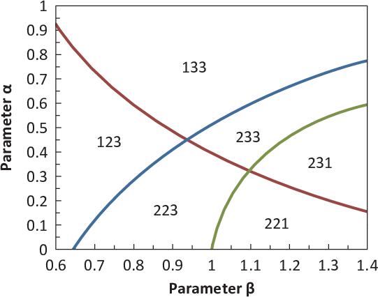
| Figure 1: Preference patterns in relation to parameters of the additive difference model for dependent gambles. This model allows six preference patterns for Triple 4 of Butler and Pogrebna (2018), including the intransitive patterns 123 and 231, depending on the power function exponents in Equation 3. |
The additive difference model (ADM), with power functions (Birnbaum & Diecidue, 2015, Equations 10 and 13), for gambles X = (x1, p1; x2, p2; x3, p3) and Y = (y1, q1; y2, q2; y3, q3), can be written:
|
ψ(X,Y) = ∑σ(xi,yj)piqj|xiα−yjα|β (3) |
where ψ(X,Y) is the decision function such that if it is positive, prefer X; if it is negative, prefer Y; α and β are parameters. σ(xi, yj) is the sign function (−1, 0, 1) that retains the sign of xi − yj. The summation in the dependent case includes only corresponding event-consequence branches (only where i=j), and the product of probabilities is replaced by the branch probabilities. In the independent case, one must sum over all possible contrasts and weight them by the appropriate product of the branch probabilities. This model is fairly general (Birnbaum & Diecidue, 2015) and can be used to represent regret theory (Loomes & Sugden, 1982) as well as advantage-seeking models, like most probable winner.
The ADM model, assuming independence, can imply the intransitive pattern, 123, as well as the patterns 133, 233, and 223. To test between the independent and dependent interpretations of these regret-type models experimentally, one could manipulate permutations of the consequences over events: the dependent model implies intransitive cycles should be reversible, an implication called "recycling" by Birnbaum and Diecidue (2015), whereas the independent model implies no effects of permuting the consequences over equally likely events or positions. If I understand their method, Butler and Pogrebna (2018) always presented the consequences in in the same positions, so no tests of permutation or recycling were provided in their study.
As shown in Figure 1, the ADM model for dependent gambles can handle six preference patterns (123, 133, 233, 231, 221, and 223). The intransitive pattern of 123 occurs, for example, when α = 0.4, β=0.7, and the opposite intransitive cycle, 231, is implied by parameters with a "regret" interpretation (Loomes & Sugden, 1982); that is, when β > 1; e.g., α = 0.4, β=1.3. This model can also handle the transitive, 221 pattern that is the most probable preference pattern overall in the study (Table 2). This model is quite flexible, allowing so many possible patterns; it rules out only the 121 and 131 response patterns. The strongest evidence against it in these data appears in Triple 9, where 8 people showed the 121 pattern on both repetitions, and 17% are estimated (Table 2) to have this true preference pattern.
The additive difference model implies the property of restricted branch independence, which was significantly violated in Birnbaum and Diecidue (2015) and other studies, but was not tested in Butler and Pogrebna (2018). Thus, a skeptic might not be impressed by the fact that this model, which can handle so many different preference orders, remains compatible with these data.
Many other theories could be (or have been) devised to make predictions for this study, besides those listed in Table 4. Therefore, I prefer to say that evidence of any subset of preference patterns is "consistent with" rather than "supports" a theory. Some theories are more flexible (allow more possible preference patterns) than others. Although some people like to compare models by statistical computations of fit adjusted for a model’s complexity in a single study, I do not favor that approach. I prefer to compare theories by their success in predicting the results of new tests of diagnostic properties, where the rival theories make qualitatively different predictions. Further comments on testing and comparison of models like these are in Birnbaum (2019).
References
Birnbaum, M. H. (2008). New paradoxes of risky decision making. Psychological Review, 115, 463–501.
Birnbaum, M. H. (2012). A statistical test of the assumption that repeated
choices are independently and identically distributed. Judgment and
Decision Making, 7, 97-109
Birnbaum, M. H. (2013). True-and-error models violate independence and yet they are testable. Judgment and Decision Making, 8, 717–737.
Birnbaum, M. H. (2019). Bayesian and frequentist analysis of True and Error models. Judgment and Decision Making, 14(5), 608–616.
Birnbaum, M. H., & Bahra, J. P. (2012). Testing transitivity of preferences in individuals using linked designs. Judgment and Decision Making, 7, 524–567.
Birnbaum, M. H. & Bailey, R. (1998). Decision models- TAX and CPT calculator. WWW document, viewed May 6, 2020.
http://psych.fullerton.edu/mbirnbaum/calculators/taxcalculator.htm
Birnbaum, M. H., & Diecidue, E. (2015). Testing a class of models that includes majority rule and regret theories: Transitivity, recycling, and restricted branch independence. Decision, 2, 145–190.
Birnbaum, M. H., & Gutierrez, R. J. (2007). Testing for intransitivity of preference predicted by a lexicographic semiorder. Organizational Behavior and Human Decision Processes, 104, 97–112.
Birnbaum, M. H., Navarro-Martinez, D., Ungemach, C., Stewart, N. & Quispe-Torreblanca, E. G. (2016). Risky decision making: Testing for violations of transitivity predicted by an editing mechanism. Judgment and Decision Making, 11, 75–91.
Birnbaum, M. H., & Quan, B. (2020). Note on Birnbaum and Wan (2020): True and error model analysis is robust with respect to certain violations of the MARTER model. Judgment and Decision Making, 15(5), 861–862.
Birnbaum, M. H., & Quispe-Torreblanca, E. G. (2018). TEMAP2.R: True and error model analysis program in R. Judgment and Decision Making, 13(5), 428–440.
Birnbaum, M. H., & Schmidt, U. (2008). An experimental investigation of violations of transitivity in choice under uncertainty. Journal of Risk and Uncertainty, 37, 77–91.
Birnbaum, M. H., & Wan, L. (2020). MARTER: Markov true and error model of drifting parameters. Judgment and Decision Making, 15, 47–73.
Butler, D. J., & Blavatskyy, P. (2020). The voting paradox... with a single voter? Implications for transitivity in choice under risk. Economics & Philosophy, 36, 61–79.
Butler, D. J., & Pogrebna, G. (2018). Predictably intransitive preferences. Judgment and Decision Making, 13, 217–236.
Fishburn, P. C. (1991). Nontransitive preferences in decision theory. Journal of Risk and Uncertainty, 4, 113–134.
Lee, M. D. (2018). Bayesian methods for analyzing true-and-error models. Judgment and Decision Making, 13(6), 622–635.
Loomes, G., & Sugden, R. (1982). Regret theory: An alternative theory of rational choice under uncertainty. The Economic Journal, 92, 805–824. http://dx.doi.org/10.2307/2232669
McNamara J. M., Trimmer P. C., & Houston A. I. (2014). Natural selection can favour ‘irrational’ behaviour. Biology Letters, 10, 20130935.
http://dx.doi.org/10.1098/rsbl.2013.0935
Regenwetter, M., Dana, J., & Davis-Stober, C. P. (2011). Transitivity of
preferences. Psychological Review, 118, 42–56.
Schramm, P. (2020). The individual true and error model: Getting the most out of limited data. Judgment and Decision Making, 15(5), 851–860.
Sopher, B., & Gigliotti, G. (1993). Intransitive cycles: Rational Choice or random error? An answer based on estimation of error rates with experimental data. Theory and Decision, 35, 311–336
This document was translated from LATEX by
HEVEA.