Judgment and Decision Making, Vol. 15, No. 4, July 2020, pp. 572-585

Judgments of a treatment’s effectiveness are usually biased by the probability with which the outcome (e.g., symptom relief) appears: even when the treatment is completely ineffective (i.e., there is a null contingency between cause and outcome), judgments tend to be higher when outcomes appear with high probability. In this research, we present ambiguous stimuli, expecting to find individual differences in the tendency to interpret them as outcomes. In Experiment 1, judgments of effectiveness of a completely ineffective treatment increased with the spontaneous tendency of participants to interpret ambiguous stimuli as outcome occurrences (i.e., healings). In Experiment 2, this interpretation bias was affected by the overall treatment-outcome contingency, suggesting that the tendency to interpret ambiguous stimuli as outcomes is learned and context-dependent. In conclusion, we show that, to understand how judgments of effectiveness are affected by outcome probability, we need to also take into account the variable tendency of people to interpret ambiguous information as outcome occurrences.

Keywords: illusion of causality, outcome-density, contingency learning

1  Introduction

Most decisions that we make every day are based on causal knowledge. For example, we could take a painkiller because we think that it will help us reduce our headache; or we could use the seatbelt when driving, in the belief that it will prevent damage in case of car accident. These are decisions that imply a causal link between two types of events: causes (taking a pill, using the seatbelt) and effects or outcomes (symptomatic relief, damage prevention). Since decisions of this kind could be of high relevance for our survival or quality of life, it would be desirable that the causal beliefs that guide them are accurate. However, as we will later explain, this is not always the case: people could insist on taking a completely ineffective treatment (pseudomedicine) because they erroneously believe it has beneficial effects; or they could decide not to use the seatbelt because they fail to see the preventive causal link between this safety measure and accidental damage. Thus, it is important to conduct research on how causal knowledge can be biased, and on the individual differences that explain why some people could be more prone to errors.

In this research endeavor, we need first to address how causal beliefs are formed through the process of causal learning. This often involves learning the contingency, or statistical correlation, between the potential cause and the outcome. One of the many ways in which this contingency information can be obtained is from the direct experience with both events. For the simplest case, with only one cause and one outcome, and assuming that both variables are binary (either they occur or they do not), there are four possible events that one can experience: type a trials (both the cause and the outcome occur), type b trials (the cause occurs, but the outcome does not), type c trials (the cause, but not the outcome, occurs), and type d trials (neither occurs). These types of trial (a, b, c, and d) could appear with different frequencies. One could use this information to compute an index of contingency, such as Δ P (Allan, 1980; see alternative rules in Perales & Shanks, 2007):

As Equation 1 shows, the index assesses the difference between two conditional probabilities: the probability of the outcome conditional on the presence of the cause, P(O|C), and the probability of the outcome conditional on the absence of the cause, P(O|¬ C). If the outcome is more likely to appear in the presence of the potential cause than it is in the absence of the potential cause, then the Δ P index will take a positive value, indicating that there is some degree of contingency between the two events, and suggesting a causal link. For example, if a given food item produces allergic symptoms, one would observe that the allergic reaction appears more often after taking the food than after not taking it. A negative value of Δ P indicates the opposite relationship: P(O|C) is smaller than P(O|¬ C). For example, the probability of serious damage in case of car accident is smaller when one uses the seatbelt than when one does not. Finally, and what is more relevant for our study, there are situations in which both probabilities are equal, thus yielding a Δ P value of 0. This is a null contingency setting that normally implies the absence of a causal link. For example, using a pseudoscientific treatment for a serious disease will probably not improve the chances of healing as compared to when no treatment, or a placebo, is taken (Yarritu, Matute & Luque, 2015).

A great deal of evidence indicates that people (and other animals) are capable of detecting contingency, and that they can use this information for making causal judgments and decisions (Baker, Mercier, Vallée-Tourangeau & Frank, 1993; Blanco, Matute & Vadillo, 2010; Rescorla, 1968; Shanks & Dickinson, 1988; Wasserman, 1990). However, research has documented some factors that bias contingency estimations, particularly in null contingency settings. Perhaps the most widely studied of these biases is the outcome-density effect (OD): Given a fixed (usually null) contingency value, judgments will systematically increase above zero when the marginal probability of the outcome, P(O), is high, compared to when it is low (Alloy & Abramson, 1979; Buehner, Cheng & Clifford, 2003; Moreno-Fernández, Blanco & Matute, 2017; Musca, Vadillo, Blanco & Matute, 2010). This is a robust effect that has been replicated, and that could lead to causal illusions (perception of causal links in situations in which there is none; see for review Matute et al., 2015; Matute, Blanco & Díaz-Lago, 2019). These mistaken beliefs could, in turn, entail serious consequences, as they could underlie illusions of effectiveness of pseudoscientific medicine (Matute, Yarritu & Vadillo, 2011), and contribute to maintain social prejudice (Blanco, Gómez-Fortes, & Matute, 2018; Rodríguez-Ferreiro & Barberia, 2017).

Given the importance of understanding both accurate and biased contingency detection to make sense of people’s causal beliefs and decisions, it would be useful to find out whether some individuals are more likely to bias their judgments than others. Consequently, many researchers in the field of contingency learning have shifted their interest toward finding evidence for individual differences in contingency detection (Byrom, 2013; Byrom & Murphy, 2017; Sauce & Matzel, 2013). Thus, we know that people differ in their sensitivity to the OD effect. For example, while the OD bias seems quite prevalent in the general population, people with mild dysphoria are more resistant to this manipulation (i.e., depressive realism, Alloy & Abramson, 1979; Msetfi, Murphy & Simpson, 2007). Believers in the paranormal can also show stronger OD biases when facing a contingency learning task on an unrelated domain (Blanco, Barberia & Matute, 2015; Griffiths, Shehabi, Murphy & Le Pelley, 2018). Additionally, people can selectively display a stronger/weaker OD bias depending on the content of the materials, and how it contradicts/reaffirms their previous attitudes (Blanco et al., 2018). Finally, even more subtle differences such as assuming a higher or lower base-rate for the outcome can in fact modulate the OD bias, making it stronger or weaker, because the actual P(O) observed during the experiment can be interpreted as high or low depending on the one that was previously assumed (Blanco & Matute, 2019).

1.0.1  When the OD (outcome-density) bias depends on our interpretation

The study we have just mentioned (Blanco & Matute, 2019) illustrates that people who receive identical or similar information (a null contingency made up of a sequence of type a, b, c, and d trials) can produce weaker OD biases when they interpret that the P(O) they observed is actually lower than the one they should expect (Experiment 1). Additionally, they also would produce the opposite, stronger OD biases, when they judge that the P(O) they saw is higher than they were expecting (Experiment 2). That is, not only the actual level of P(O) matters for developing the OD bias, but the interpretation that the participant makes is also important.

This opens the question of whether all people tend to interpret outcome occurrences in the same way, when it comes to learning a contingency or grasping a potential causal relationship. In real life, it is often not clear when an outcome has occurred. Consider a person who is treating his/her common cold with a treatment. At the beginning of the treatment, the symptoms are intense and easy to recognize. However, as the disease resolves and health improves, symptoms become less severe, making them sometimes difficult to detect or categorize as such: If I cough less frequently today than I did yesterday, I could either interpret it as a healing (i.e., an outcome occurrence), or instead focus on the fact that I am still coughing, so I am not completely healed (that is, a no-outcome trial). Note that depending on my interpretation of what counts as an outcome, the overall P(O) that I will experience will likely be very different, and the contingency may also be affected. Thus, the interpretation of outcome information can in fact determine the judgment of causality (in this case, the judgment about the effectiveness of the treatment). Therefore, this could be a potential source of individual variability in the sensitivity to the OD bias: given the same level of actual P(O), people might produce very different judgments of causality because of their interpretations of outcome events.

If different interpretations of outcome events are possible, it is because, in real life, many relevant outcomes are usually continuous (i.e., they are a matter of degree) and variable. By contrast, in the great majority of experiments, they are binary (they either occur or not) and fixed. A recent exception are the studies conducted by Chow and colleagues (Chow, Colagiuri & Livesey, 2019). In their experiments, participants rated how effective a medicine was, after seeing a series of trials in which the medicine and the outcome (healing) could either be present or not (i.e., the four trial types described above), as it is common in the literature on this topic. However, instead of presenting outcome information in a binary fashion (i.e., “present”/“absent”), they conveyed this information as a number describing the “health level” of the patient, thus creating the impression that outcomes were continuous. Additionally, trials defined as outcome-present did not always depict exactly the same health level. Instead, some random variation was added (i.e., the outcomes were variable rather than fixed). This is a more ecological setting than previously used ones, as many real-life situations (such as judging whether a treatment is working for a common cold) can be better thought as involving continuous and variable outcomes. Although this type of presentation implies that the task becomes more difficult (i.e., it is harder to ascertain whether the outcome took place or not, or whether our health is actually improving or not, if the outcome takes an intermediate value), the results clearly indicated that the OD bias appears systematically, with similar size, both in binary-fixed outcome conditions and in continuous-variable outcome conditions.

It has been hypothesized (Chow et al., 2019; Marsh & Ahn, 2009) that, when presented with the information of a continuous outcome, people spontaneously categorize this information into one of the four categories (type a, b, c, and d trials). That is, despite the information is continuous, the usual interpretation by the participant reduces it to a discrete value (either the event took place or not). Chow et al.’s (2019) study did not consider potential differences between participants in their tendency to classify a given outcome value as an outcome occurrence/absence, since this was not the aim of their research. However, as we illustrated above, these differences could exist in real-life situations involving continuous and variable outcomes (because they can be interpreted in various ways). For example, some people would subjectively interpret their 10% symptomatic remission as an outcome (i.e., healing), while others would make the opposite classification because 10% is too small a change.

---

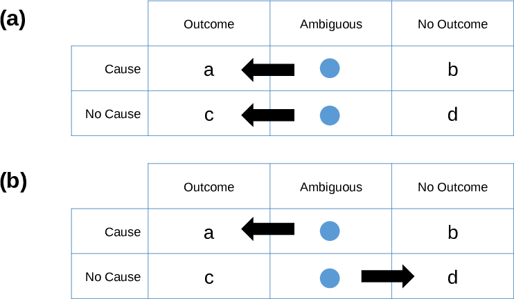
Figure 1: Two ways in which individual differences in the interpretation of ambiguous stimuli could lead to illusions of effectiveness (overestimated judgments of causality): either (a) by systematically categorizing ambiguous stimuli as outcomes (cells a and c), therefore inflating P(O), or (b) by inflating the contingency through the differential categorization of ambiguous stimuli as outcome or no outcome, depending on the presence of the cause, that is, cells a and d.

---

In this task of interpreting and classifying outcomes, perceptual processes may play an important role, as they are key to discriminating different stimuli (in this case, “outcome” vs. “no outcome”). In fact, individual differences in the tendency to detect meaningful patterns in ambiguous perceptual material have been widely documented. For example, people who believe in the supernatural and in conspiracy theories are more likely to illusorily perceive a meaningful pattern in a stimulus consisting of random clouds of dots (van Elk, 2015; van Prooijen, Douglas & De Inocencio, 2017), as it happens too to participants who feel lack of control (Whitson & Galinsky, 2008; although see Van Elk & Lodder, 2018). Similarly, patients with schizophrenia tend to produce more false-alarm errors and be overconfident when judging ambiguous visual patterns (Moritz, Ramdani, et al., 2014), a mechanism that has been linked to hallucinations and delusions, typical in this disorder. Moreover, both paranormal beliefs and schizophrenia have been associated to causal illusions of some kind (Blanco et al., 2015; Moritz, Goritz, et al., 2014; Moritz, Thompson & Andreou, 2014), including the OD bias, which might indicate a common underlying mechanism. We suggest that the tendency of these participants to interpret ambiguous patterns as outcome occurrences, thus inflating the P(O) they are factually exposed to, might be one key factor at the basis of their stronger vulnerability to causal illusions.

In this article, we describe two experiments conducted on healthy individuals. In Experiment 1, our aim was to document individual variability in the tendency to categorize ambiguous information as outcome occurrences. This variability could be important, because it can affect judgments of causality in two different ways: (a) if the tendency to categorize the stimuli as outcome or no-outcome does not depend on whether the cause is present, then those people who report perceiving the outcome more often will not experience an inflated contingency, but will nevertheless experience an inflated value of P(O) that can lead to overestimated judgments of causality (OD bias). This possibility is depicted schematically in Figure 1a. Note that, as the tendency to interpret the stimuli as outcomes is in this case not affected by the presence of the cause, the overall perceived contingency remains unchanged, because a similar proportion of ambiguous trials will be categorized as outcomes when the cause is present and when the cause is absent. On the other hand, there is a second possibility: (b) If the tendency to categorize the stimuli as outcomes is different depending on whether the cause is present or not, then participants will be effectively experiencing a different contingency from the one that was programmed, thus leading to judgments that do not match the programmed contingency (Figure 1b). For instance, people expecting the cause to produce the outcome might tend to interpret an ambiguous stimulus as an outcome more often in the presence of the cause than in its absence, which could increase the perceived contingency beyond its actual value.

In sum, we have two potential ways in which the variability in the interpretation of ambiguous stimuli could produce causal illusions: by inflating P(O), or by inflating contingency. We will first investigate which of the two predictions (Figure 1a or Figure 1b) holds in null contingency settings, which are the conditions that typically produce overestimated judgments.

2  Experiment 1

In this experiment, we aim to investigate how differences in the tendency to interpret ambiguous stimuli as “outcome” or “no outcome” could produce changes in the causal judgments. Specifically, individuals with a more liberal criterion (i.e., most stimuli are categorized as “outcome”) would experience a high subjective P(O), which would result in strong overestimations of a null contingency (OD bias). This would contrast with participants with a more conservative criterion, who would display the opposite pattern. In principle, we assume that there will not be differences in the outcome interpretation criterion depending on the presence of the cause (in line with the prediction of Figure 1a), because there is no a priori reason to expect that outcomes should appear with different probabilities depending on the cause status.

2.1  Method

2.1.1  Participants and apparatus

One hundred Psychology students (out of which 19 men) from the University of Deusto took part in Experiment 1 in exchange for course credit (with age M = 18.50 years, SD = 0.86). The experiment was conducted in a large computer room. All materials were presented in Spanish. The experimental task was implemented as a JavaScript program that can run online in most browsers, without installing any plugin or additional programs. The participants were informed before the experiment that they could quit the study at any moment by closing the browser window. The data collected during the experiment were sent anonymously to the experimenter only upon explicit permission by the participant, indicated by clicking on a “Submit” button. If the participant clicked on the “Cancel” button, the local information was erased. No personal information (i.e., name, IP address, e-mail) was collected. We did not use cookies or other software to covertly obtain information from the participants.

---

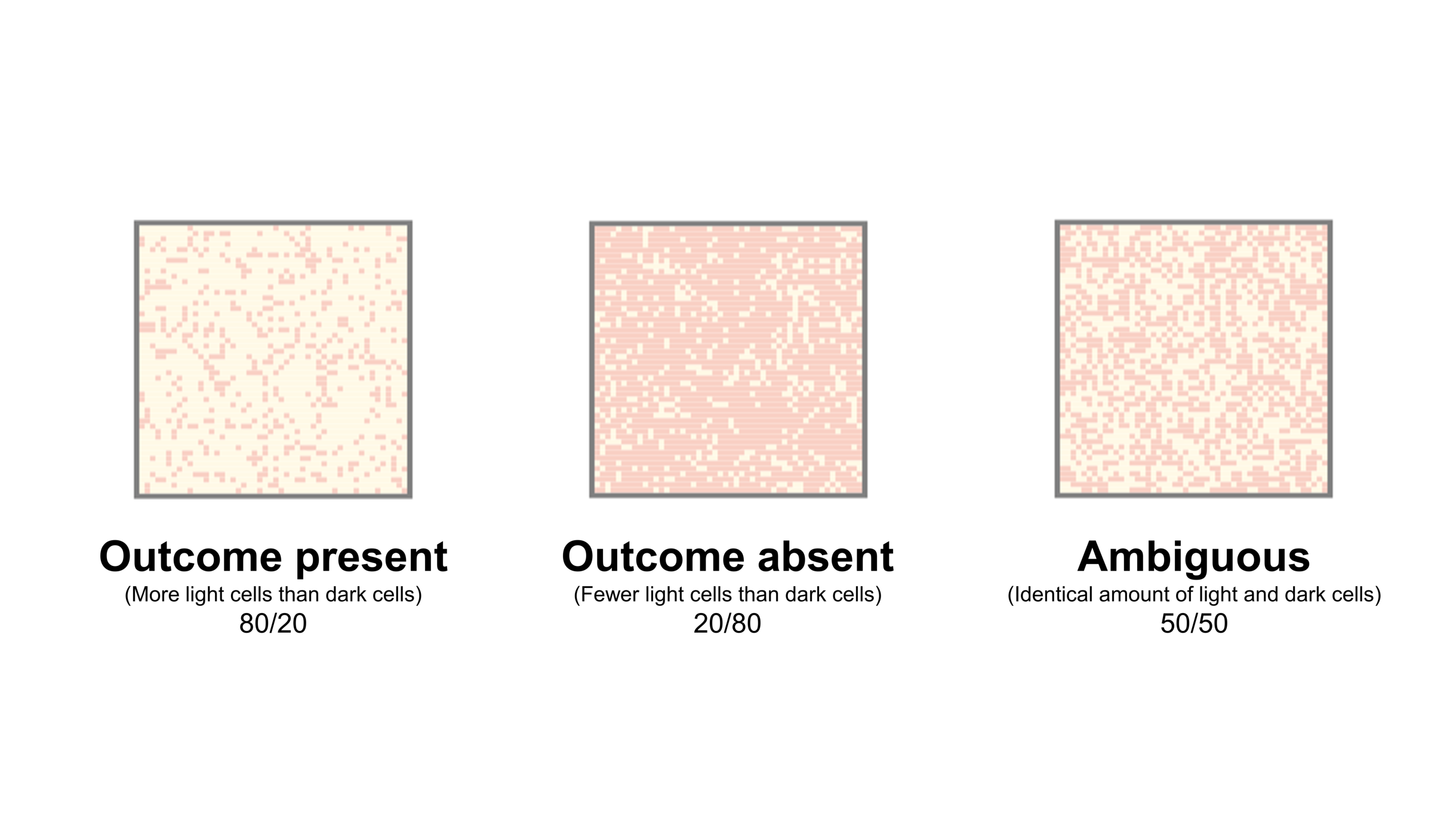
Figure 2: Examples of stimuli used in outcome-present trials (cured patient), outcome-absent trials (no cured patient), and ambiguous trials in the contingency learning task. Note that the assignment of colors (light/dark) to roles (ill/normal cells) was randomly decided for each participant, but for simplicity we present here only one of the assignments.

---

2.1.2  Procedure

Within the Method, overview of the study procedure. The experiment was designed as a standard trial-by-trial contingency learning task (Matute et al., 2015), framed in a medical scenario (a fictitious medicine, Batatrim, plays the role of potential cause, and the recovery from a disease is the outcome). However, we introduced a number of changes to adapt the task to our current purposes.

The main innovation in this procedure is in the stimuli used as outcome. On each trial, the information about the outcome was presented on a 50 x 50 pixels matrix which represents a tissue sample obtained from a given patient. The matrix contained 2500 points (i.e., cells) of two colors (dark pink and light yellow), randomly distributed in space. The proportion of light to dark cells was determined by the type of trial. The instructions stated that the Lindsay Syndrome (a fictitious disease) affects human tissues and causes some of the cells to appear in a dark color, instead of the normal light color. (Note that the assignment of dark/light colors to ill/normal cells was randomly decided for each participant, although, for simplicity, in this section we will refer only to one of the two possible assignments: dark for ill cells, and light for normal cells.) More specifically, participants were told that: (a) a patient suffering from the syndrome will present more dark cells than light cells and, conversely, that (b) when a patient has overcome the syndrome, his/her tissues will contain more light than dark cells. Thus, in outcome-present trials (i.e., a and c, when the patient is cured), there will be 2000 light cells (80%) and 500 dark cells (20%), whereas in outcome-absent trials (i.e., b and d, when the patient is not cured), the proportion will be the opposite. These proportions were decided to make the task of interpreting outcome-present and outcome-absent trials easy, because the perceptual difference between these two types of trials is notable (Figure 2, left and center).

To ensure all participants were able to acquire this discrimination correctly, we included a practice phase in which a series of eight stimuli with various level of difficulty (i.e., proportions 90/10, 80/20, 70/30, 60/40, 40/60, 30/70, 20/80, and 10/90) had to be categorized as “cured/not cured” tissue, and the appropriate feedback was then provided. If participants failed to categorize more than two out of these eight stimuli, they were forced to continue the practice phase until they achieved at least six out of eight correct classifications (i.e., 75%).

---

Table 1: Frequencies of each type of trial in the contingency learning phase of Experiment 1.

	Outcome present (cured)	Ambiguous Outcome	Outcome absent (not cured)
Cause present (Medicine was taken)	5	10	5
Cause absent (Medicine was not taken)	5	10	5

---

Once the practice phase was over, participants underwent the learning phase. During the contingency learning phase there was an additional type of trial, which presented an ambiguous outcome with as many light cells as dark cells (Figure 2, right). This stimulus (50/50) cannot be objectively interpreted as cured (outcome) or not cured (no outcome), because it lies exactly in the middle between cured and not cured tissues. Therefore, there could be individual differences in interpretation of ambiguous trials: participants with a conservative criterion would interpret most ambiguous stimuli as outcome-absent, whereas those with a liberal criterion would interpret them as outcome-present. Additionally, participants could, to some extent, tend to categorize the ambiguous stimulus as outcome or not depending on whether the cause (medicine) is present, as explained in the Introduction.

Table 1 contains the frequencies of each type of trial presented in the contingency learning phase. Attending to non-ambiguous trials, the contingency between taking the medicine and healing was null, since the probability of overcoming the syndrome was identical both in the presence and in the absence of the medicine, i.e., P(O|C) = P(O|¬ C) = 0.50. However, the interpretation of ambiguous trials could affect this computation: for example, if participants tend to categorize or interpret the ambiguous stimuli as “outcome” more often in the presence of the cause than in its absence, then the actually perceived contingency would become positive, P(O|C) > P(O|¬ C) (see, e.g., Figure 1b). The 30 trials were arranged in random order for each participant.

---

Figure 3: Screenshot of one trial in the contingency learning task. On the left-hand of the screen, participants see the information about the cause and outcome statuses. Then, on the right-hand, they must categorize the status for both cause and outcome.

---

The distribution of non-ambiguous trial frequencies depicted in Table 1 was chosen to optimize the information provided by our study. Since we aimed to examine the spontaneous tendency to categorize ambiguous stimuli as outcomes in a null contingency setting, the frequencies of all four types of non-ambiguous trials were set to be identical, i.e., P(O) = P(C) = 0.50. This ensures that for all participants, non-ambiguous trials provide the same information: a null contingency between the cue and the outcome and a medium level of P(O) and P(C). Any deviation from these frequencies, such as a P(O) > 0.50, could introduce a bias as it could affect the tendency to categorize ambiguous stimuli (Experiment 2 will deal with one of these situations).

To assess the tendency to categorize the stimuli, the contingency learning task included two questions in each trial (see a sample of a trial in Figure 3). The instructions to this phase asked the participants to help the researchers classify each record in a fictitious study that was conducted to test the effectiveness of the medicine. On each trial, the information about the cause (medicine) and outcome (tissue) appeared on the left hand of the screen (e.g., “This patient took Batatrim; This is the tissue sample”). Then, participants had to indicate, in this order: (a) whether the patient took Batatrim or not (i.e., thus categorizing the cause status), and then (b) whether the outcome occurred or not (i.e., thus categorizing the outcome status). A reminder of the correct interpretation of dark/light cells was provided (Figure 3) to help in the task, but no feedback was given during this phase. Although we were interested only in the interpretation of outcomes, because categorizing the cause status was trivial in this task, we included both questions to prevent participants from focusing too much on outcomes and overlook the causes. The responses to the outcome categorization were recorded for all trials (0: no outcome; 1: outcome), thus allowing us to compute a subjective P(O) index: the number of outcomes categorized as “outcome” over the total number of trials. Additionally, we also computed the subjective contingency index, which is obtained by applying the Δ P rule to the trial frequencies, after recoding them according to the categorization (i.e., if the ambiguous stimulus in a cause-present trial is categorized as “outcome”, then it counts as a “type a” trial, and so on). Both subjective P(O) and subjective contingency could affect the perceived contingency between medicine and healings.

After the sequence of thirty trials, participants were asked to rate the extent to which the medicine, Batatrim, was able to heal the syndrome (i.e., a causal judgment), as is typical in these tasks. The judgment was collected on a scale from 0 (not effective at all) to 50 (quite effective) to 100 (completely effective). Given that the actual contingency, considering non-ambiguous trials, was set to null, the correct answer should be zero. However, some participants could show a causal illusion (i.e., an overestimation of the causal relationship), as revealed by a higher judgment, as is usual in previous experiments with this type of task (Alloy & Abramson, 1979)¹.

2.2  Results and discussion

2.2.1  Categorization of non-ambiguous stimuli (attention checks)

First, we used the practice phase to ensure participants were able to learn the categorization rule. All participants were able to successfully meet the practice phase criterion to continue to the contingency learning phase at their first attempt (i.e., all answered more than six items correctly): 83% of participants answered all eight practice trials correctly, and 17% missed only one out of eight trials. Then, we examined the number of mistakes made in the categorization of causes and outcomes in non-ambiguous trials during the contingency learning phase. Most participants committed none or few mistakes. When categorizing outcomes in non-ambiguous trials, 93% of participants did not make any mistake, 99% made 4 or fewer, and only one participant showed an extreme behavior with 20 mistakes out of 20 non-ambiguous trials. This suggests that this individual interpreted the task backwards (all outcomes were understood as no-outcomes and vice versa, despite solving successfully the practice phase, and probably ignoring all written messages that reminded the correct meaning of the light/dark cells). In comparison, categorizing the causes led to more errors, but still 65% of the sample did not make any mistake, and 95% made 5 or fewer. The task of categorizing the cause status was actually very easy (i.e., it consisted of just repeating the information that was still available on the screen, as Figure 3 indicates), but perhaps the focus on outcome categorization drew the attention away from the cause information, so that participants can inadvertently click on the wrong answer.

---

Table 2: Descriptive statistics for the variables in the contingency learning phase in Experiment 1.

	Non-ambiguous trials		Ambiguous trials		All trials
Variable	M	SD	M	SD	M	SD
Subjective P(O)	0.497	0.023	0.430	0.377	0.464	0.189
Subjective P(O|C)	0.496	0.025	0.446	0.378	0.471	0.190
Subjective P(O|¬ C)	0.498	0.029	0.415	0.391	0.456	0.196
Subjective Contingency	−0.002	0.029	0.031	0.156	0.014	0.081

---

In this experiment, mistakes in the categorizing of outcomes in particular can be problematic because, if participants are not correctly understanding what counts as an outcome in a non-ambiguous trial, our assessment of the interpretation of ambiguous trials could be compromised and strongly affect our conclusions. Guided by this reasoning, we decided that an a priori exclusion criterion was necessary: As a result, we excluded six participants who made more than five mistakes in both cause and outcome classifications (out of 30 trials) in the whole session, which could indicate that they either were not paying attention, or did not understand the instructions. Thus, the final sample consisted of N = 94 participants. Note that an alternative approach is to not exclude any participant, but including the number of errors as a covariate, which produces essentially the same conclusions that we report below.

2.2.2  Categorization of ambiguous stimuli

Table 2 depicts the descriptive statistics for the variables assessed in the experiment: subjective P(O), subjective P(O) conditional on the cause status (present or absent), and subjective contingency. These were computed for both ambiguous and non-ambiguous trials.

We have previously described how participants classified the stimuli shown in non-ambiguous trials. As expected, the task was solvable, and most participants made no mistakes. This implies that in non-ambiguous trials the performance was very close to perfect, and the P(O) computed from these trials is almost a constant in our sample (note the SDs values are all around zero in Table 2). However, we expected that people could vary from each other in their interpretation of the stimuli in ambiguous trials.

---

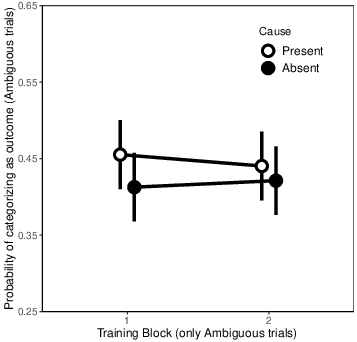
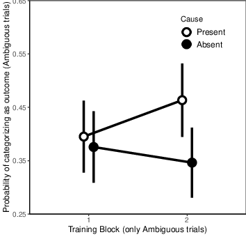
Figure 4: Probability of categorizing the ambiguous stimulus as “outcome” for both cause-present and cause-absent trials, divided by training block (two blocks of 5 trials) in Experiment 1. Error bars depict 95% confidence intervals for the mean.

---

By examining the subjective P(O) for ambiguous stimuli (Table 2), we infer that the criterion used to categorize these ambiguous stimuli was slightly conservative, as the mean values were all below 0.50. This means that, when presented with an ambiguous stimulus, participants tended to classify it as a non-healed sample of tissue rather than as a healed one. However, the criterion is still close to 0.50, indicating that this preference in the classification is small. Additionally, there are no apparent differences between the probability of reporting an ambiguous stimulus as a healing in the presence of the cause, P(O|C), and in the absence of the cause, P(O|¬ C). That is, it seems that people did not change their classification criterion for ambiguous stimuli as a function of whether the medicine was taken or not (Table 2, column for ambiguous trials).

To test these impressions and examine the potential differences in categorization of ambiguous stimuli depending on whether the cause was present or not, we conducted a repeated measures 2 (Cause: present/absent) x 2 (Blocks of 5 trials) ANOVA on the categorization decisions of ambiguous trials. This resulted in no main effect of Block (F(1, 93) = 0.021, p = 0.885, partial η² < 0.001), no main effect of Cause (F(1, 93) = 3.301, p = 0.072, partial η² = 0.034), and no interaction (F(1, 93) = 0.533, p = 0.466, partial η² = 0.006; see Figure 4). In sum, participants displayed a similar, slightly conservative, criterion to categorize the ambiguous stimuli in the presence and in the absence of the cause, which means that they were exposed to very small deviations from the null contingency. This aligns with the value of subjective contingency for ambiguous trials, reported in Table 2, which is very close to zero.

---

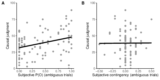
Figure 5: Scatter plot showing the relationship between causal judgments and subjective P(O) (computed by taking into account only ambiguous trials), in Experiment 1.

---

2.2.3  Causal judgments

So far, we have described how people classify the stimuli presented in the task. Now, we test whether individual differences in the categorization of ambiguous stimuli can predict differences in causal judgments. In particular, we proposed that those participants with more liberal classification criteria, and therefore higher values of subjective P(O), would bias their judgments upwards.

The causal judgments showed some overestimation of the null contingency, M = 38.71, SD = 18.88. Recall that the actual contingency that was presented to participants was null, so judgments higher than zero suggest an overestimation.

Thus, we tested a regression analyses in which the subjective P(O) computed from ambiguous trials was used as a predictor of judgments. The results were significant (β = 0.322, t(92) = 3.27, p = 0.002; Figure 5). Moreover, the same effect was found for trials in which the cause was present and for trials in which the cause was absent, i.e., P(O|C) and P(O|¬ C) (β = 0.322, t(92) = 3.27, p = 0.002, and β = 0.309, t(92) = 3.12, p = 0.002, respectively).

On the other hand, subjective contingency (computed from ambiguous trials) did not significantly predict the judgments (β = 0.005, t(92) = 0.050, p = 0.960). This is not surprising, as our previous analyses showed that most participants tended to categorize ambiguous stimuli as healings as often in the presence as in the absence of the cause, that is, they did not seem to take into account whether the medicine was administered or not in their classification task. As a consequence, subjective contingency was almost a constant value (very close to zero) for almost all participants.

The previous analyses were conducted on ambiguous trials only. We have argued that, because the task of classifying non-ambiguous stimuli was very easy and the performance close to perfect (furthermore, we excluded those few participants who made more than five mistakes), values of P(O) computed from non-ambiguous trials are almost a constant value in our sample. This means that the variance in the judgments cannot be explained by these trials, so they add little information. For completeness, we report here the regression analyses with the P(O) of non-ambiguous trials only, β = −0.081, t(92) = 0.785, p = 0.435. The non-significant result suggests that the classification of non-ambiguous stimuli played no relevant role in the variance of the judgments. If we, by contrast, repeat the analyses by using all trials (combining ambiguous and non-ambiguous trials), the results are the same as above with ambiguous trials only.

3  Experiment 2

Experiment 1 served to illustrate that, when presented with ambiguous information about an outcome of interest, people can differ in their tendency to interpret such stimuli as “outcome” or “no outcome”, and that this tendency can predict a bias in their causal judgments: the more outcomes the participant has recognized during the task, the stronger the overestimation of a null contingency. Additionally, we found no evidence that people make a difference in their categorization of ambiguous outcomes as a function of whether the potential cause is present or not. That is, our results favor the hypothesis illustrated in Figure 1a.

However, Experiment 1 was conducted in a null contingency, medium P(C), medium P(O) setting. In these conditions, we were neither influencing nor biasing the spontaneous categorization criterion (i.e., there was no specific incentive to classify the stimuli in a particular way). In Experiment 2, we go one step further. We propose that the tendency to categorize outcomes is not fixed, but rather it is context-dependent. Interestingly, Marsh & Ahn (2009) showed that the categorization of ambiguous values of a causal cue as “cause” or “no cause” was affected by the perceived strength of the causal relationship. Thus, we wondered whether the tendency to categorize ambiguous stimuli as “outcome” could change if we presented a different situation in non-ambiguous trials: a positive contingency, instead of a null contingency. In a positive contingency, the probability of the outcome is higher in cause-present trials than it is in cause-absent trials. As a result, the categorization criterion for ambiguous trials could react accordingly, by becoming more lenient in cause-present trials, and more conservative in cause-absent trials (this prediction is depicted in Figure 1b). This is due to the well-known effect of expectations on the classification criterion (Bang & Rahnev, 2017). The change in the criterion depending on the cause status would then produce a deviation in the subjective contingency in ambiguous trials (it would become positive instead of undetermined), and in turn could exert an effect on causal judgments: the higher the subjective contingency, the stronger the overestimation. Thus, Experiment 2 was designed with the aim of testing whether the prediction in Figure 1b is possible by providing a positive contingency context in the non-ambiguous trials.

---

Table 3: Frequencies of each type of trial in the contingency learning phase in Experiment 2.

	Outcome present (cured)	Ambiguous Outcome	Outcome absent (not cured)
Cause present (Medicine was taken)	14	10	1
Cause absent (Medicine was not taken)	1	10	14

---

3.1  Method

3.1.1  Participants and apparatus.

Forty-one Psychology students (including 4 men) took part in Experiment 2 in exchange for course credit (with age M = 18.60 years, SD = 1.26), in conditions similar to those of Experiment 1. As some of the participants were exchange students from other countries, participants were given the option to choose the language (Spanish, English) in which they preferred to do the study. All but 4 chose to do the experiment in Spanish.

3.1.2  Procedure.

The procedure was identical to that of Experiment 1, except for the trial frequencies (see Table 3). From the numbers of the table, we can compute P(O|C) = 14/(14+1) = 0.93, and P(O|¬ C) = 1/(1+14) = 0.07, which yields a contingency of Δ P = 0.86 (a positive, high value that suggests a strong causal relationship).

3.2  Results and Discussion

---

Table 4: Descriptive statistics for the variables in the contingency learning phase in Experiment 2.

	Non-ambiguous trials		Ambiguous trials		All trials
Variable	M	SD	M	SD	M	SD
Subjective P(O)	0.749	0.008	0.395	0.350	0.458	0.139
Subjective P(O|C)	0.931	0.010	0.429	0.363	0.731	0.144
Subjective P(O|¬ C)	0.067	0.000	0.361	0.353	0.184	0.141
Subjective Contingency	0.864	0.010	0.068	0.154	0.546	0.062

---

3.2.1  Categorization of non-ambiguous stimuli (attention checks).

As in Experiment 1, all participants successfully reached the learning criterion in the practice phase: 89.5% of participants made no errors in this phase, while 10.5% made one error, indicating that the discrimination was correctly acquired. Once in the contingency learning phase, all but one participant made no mistakes in the outcome categorization for non-ambiguous trials, and the remaining participant made only one mistake. Also, as we saw in Experiment 1, categorizing the cause status produced more errors. In this experiment, 78% of the sample made no mistakes. No participant made more than five mistakes in their categorizations of cause and outcome (combined) during the contingency learning phase, which was our exclusion criterion (the same used in Experiment 1). Consequently, there were no exclusions in this study.

---

Figure 6: Probability of categorizing the ambiguous stimulus as “outcome” for both cause-present and cause-absent trials, divided by training block (two blocks of 5 trials) in Experiment 2. Error bars depict 95% confidence intervals for the mean.

---

3.2.2  Categorization of ambiguous stimuli.

We depict the descriptive statistics of the main dependent variables of the contingency learning phase in Table 4. Given that there were few categorization mistakes in non-ambiguous trials, the values of subjective P(O) and subjective contingency in these trials were very close to the programmed values, with small standard deviations. Thus, we move on to describing ambiguous trials. Overall, the classification criterion was conservative in ambiguous trials, as P(O) was lower than 0.50 (i.e., participants tended to report ambiguous stimuli as no-outcome, or non-healed tissue, as in Experiment 1). However, unlike in Experiment 1, there seems to be a difference in the criterion depending on the cause status: the probability of reporting an outcome (healing) when classifying an ambiguous stimulus was higher when the cause was present than when it was absent, that is, P(O|C) > P(O|¬ C), thus mirroring what happened in non-ambiguous trials (Table 4). This was confirmed by statistical analyses: t(40) = 2.84, p = 0.007, d = 0.443.

To ensure that this difference is reliable, we tested the same model as in the previous experiment, by conducting a repeated measures 2 (Cause: present/absent) x 2 (Blocks of 5 trials) ANOVA on the categorization decisions in ambiguous trials (Figure 6). The main effect of Block was not significant (F(1, 40) = 0.399, p = 0.531, partial η² = 0.01). However, the main effect of Cause was significant (F(1, 40) = 8.062, p = 0.007, partial η² = 0.17), as well as the Block x Cause interaction, F(1, 40) = 4.422, p = 0.042, partial η² = 0.10. The interaction can be interpreted as follows: There is no evidence for differences between cause-present and cause-absent trials at the beginning of the training phase (Block 1; t(40) = 0.662, p = 0.512, d = 0.10), but this turns into a significant difference in Block 2 (t(40) = 3.169, p = 0.003, d = 0.495), when the training has advanced. As expected, this difference is in line with the positive contingency that was presented in non-ambiguous trials: participants tended to categorize the ambiguous stimulus as outcome more often in cause-present trials than in cause-absent trials. This was the prediction depicted in Figure 1b. Interestingly, the interaction suggests that this differential criterion depending on the cause status is the result of learning during the task: in Block 1, the criteria for cause-present and cause-absent trials are similar to each other and to those in Experiment 1 (null contingency). However, the exposure to a positive contingency ends up biasing the criteria to match the contingency.

3.2.3  Causal judgments.

Causal judgments were overall high, M = 58.41 (SD = 19.73), in line with the contingency programmed in non-ambiguous trials (Δ P = 0.86). Next, we examined the possibility that individual differences in either subjective P(O) or subjective contingency could affect the judgments. First, we focused on ambiguous trials only: A regression analysis showed that, unlike in Experiment 1, subjective P(O) was not a significant predictor of judgments, β = 0.025, t(39) = 0.159, p = 0.874. That is, the tendency to categorize ambiguous stimuli as outcomes did not predict the causal estimation. Additionally, the subjective contingency measure did not predict the judgments either, β = 0.026, t(39) = 0.161, p = 0.873.

In general, it is reasonable that none of the variables predict the causal judgments, because in this experiment the actual contingency is clearly positive thanks to the non-ambiguous trials, which makes the contribution of ambiguous trials to the judgment almost negligible: participants experienced, if anything, very small divergences from the contingency programmed in non-ambiguous trials.

The same models were tested for non-ambiguous trials only: subjective P(O) in non-ambiguous trials did not significantly predict the judgments (β = 0.068, t(39) = 0.427, p = 0.671); and neither did subjective contingency (β = 0.068, t(39) = 0.427, p = 0.671). Remember that there was little variability in these trials as the classification performance was close to perfect. (Also, the number of participants is small.) As in Experiment 1, repeating the same analyses on all trials (by combining ambiguous and non-ambiguous trials) produces the same result as with ambiguous trials.

4  General Discussion

Individual variability in perceptual abilities or in the tendency to interpret stimuli could be relevant to improve our understanding of the OD bias, and perhaps to help us ascertain why some people could be more vulnerable to its effects. This possibility has not been directly considered in previous research, to the best of our knowledge. Therefore, we decided to conduct the two experiments reported here. First, Experiment 1 used a continuous outcome (but presented in a very different fashion from Chow et al., 2019) in a learning task in which the contingency was set to zero. That is, the fictitious medicine was unable to make any change in the healthiness of tissues. Additionally, we also presented ambiguous trials in which the outcome value was intermediate, thus making the classification as outcome/no-outcome unsolvable. Participants showed differences in their tendency to classify these ambiguous trials. These differences led to variability in the subjective P(O) that they experienced during the training session, which resulted in higher judgments of causality for those participants with higher subjective P(O) values. This is a first demonstration that the OD bias can be intensified when outcomes are continuous and people display a lenient classification criterion, thus considering most ambiguous stimuli as outcome occurrences.

Then, in Experiment 2, we explored an additional possibility: that the tendency to make the categorization is actually the result of learning, or at least that it is sensitive to the information presented during the task. Indeed, when we presented a positive, rather than null, contingency between the cause and the outcome in non-ambiguous trials, participants ended up developing a differential categorization criterion for ambiguous trials depending on whether the potential cause was present or not. That is, they tended to classify ambiguous stimuli as outcome more often in cause-present trials than in cause-absent trials. This differential criterion took some time to develop, though, as it appeared only by the second block of training trials.

It is possible to interpret this change in the classification criterion as a rational reaction to ambiguous stimuli in positive contingency settings, rather than as a bias. If participants learn that cause and outcome (medicine and healing) are positively associated by looking at non-ambiguous trials, as it happens in Experiment 2, then it makes sense for them to adjust the criterion for cause-present and cause-absent trials differentially, to match the probabilities they are being showed in non-ambiguous trials. Whether rational or biased, this classification criterion leads to a higher exposure to type a and type d trials, i.e., confirmatory evidence, thus increasing the effective contingency experienced by the participant.

However, whereas in Experiment 1 judgments were consistently predicted by the subjective P(O), therefore showing an OD bias, in Experiment 2 we found no evidence for this relationship between P(O) and judgments. In principle, we would have predicted that either subjective P(O), or subjective contingency, should predict the judgments in both experiments, so the results of Experiment 2 are not completely in line with our expectations. We could interpret this null result in the following way: since Experiment 2 takes place on a less ambiguous setting (i.e., clearly positive, rather than null contingency), people’s judgments could be more directly driven by the information contained in non-ambiguous trials, leaving too small a room for the interpretation of ambiguous trials to play a relevant role (i.e., a ceiling effect). In fact, previous research with the traditional task (binary, easy to discriminate outcomes) indicated that OD biases are almost always reported, to the best of our knowledge, with null contingencies. For example, the classic study by Allan and Jenkins (1980) showed that the overestimation of contingency due to high levels of P(O) appeared only under null contingency settings, but not under positive contingency settings. It is possible that judgments in positive contingency conditions could display a ceiling effect that prevents the influence of other factors, such as subjective P(O). In sum, Experiment 2 shows that categorization tendencies can be acquired by examining contingency, and can become dependent on the cause status (i.e., by changing the criterion depending on whether the cause is present), but does not provide evidence that such tendencies affect judgments in a positive contingency situation. Future experiments could try to further investigate this possibility by, perhaps, using lower contingencies for non-ambiguous trials, thus trying to avoid potential ceiling-effects.

Our current research is one of the few exploring causal learning on continuous dimensions. Traditionally, contingency learning paradigms show the information in a discretized format, that is, causes and outcomes can either be present or absent. Our procedure, by contrast, presents stimuli that differ along a continuum (from high proportion of dark cells to low proportion of dark cells). Thus, we can think of outcomes as continuous in this sense. However, both the cover story and the procedure itself try to convey the idea that outcomes must be treated as dichotomous. That is, the participant must make a decision as to whether a given tissue sample is healed or not. The implication is that there must be a “threshold” in the outcome continuum that allows a binary classification, and that this threshold can vary between different participants and conditions. This allows us to interpret the task in a way that is highly comparable with most experiments in contingency learning (as, for instance, the rule to compute contingency stays the same). In sum, although the stimuli that we used in these experiments can be understood as continuous, in fact the task worked the same way as in the traditional, binary case.

On the other hand, other experiments have previously tried to study causal and contingency learning with truly continuous causes and outcomes, and thus they deserve some comment here. For example, some authors have investigated causal learning from time series data (Davis et al., 2020; Soo & Rottman, 2018). In this type of paradigm, participants monitor the changes and fluctuations of a variable in real time. This variable plays the role of the outcome, and it could represent anything from the price of stocks to the hormone levels of a patient. Then, participants are given the opportunity to intervene on the system (Davis et al., 2020) and see the effect in real time. Generally, this type of task is known as a “dynamic system”, because the observed values are non-stationary, so that contingency becomes hard to assess. Thus, this research deals with a situation that, although representative of many real-life situations, departs clearly from the simplistic discrete scenario that we depicted in the Introduction. Another approach to continuous outcomes that is more closely related to our research is that developed by Chow et al. (2018), and that we described above. In Chow et al.’s experiments, the cause status was binary, as usual in this literature, but outcomes were presented in numerical format, thus conveying the idea of a continuum. However, they selected the values of these outcomes so that it was still possible to set a threshold (albeit arbitrary) to determine, in a binary fashion, whether the cause was followed by an outcome (i.e., high value) or not (low value). By making use of this task with continuous outcomes, Chow et al. (2018) were able to document and replicate the OD bias.

We must mention one caution when interpreting our experiments. Here, we used unidirectional response scales to collect the judgments, from 0 (the medicine has no effect) to 100 (the medicine is perfectly effective), whereas the contingency index Δ P can take on negative values to represent preventative scenarios. Thus, many researchers advocate bidirectional scales, from −100 (the medicine is perfectly effective in worsening the disease) to +100 (the medicine is perfectly effective in healing the disease). Although it is true that bidirectional scales capture better the bidirectional nature of contingency, and might change the participants’ answers (Neunaber & Wasserman, 1986), we argue that they do not come without problems. To begin with, many participants find it hard to interpret a bidirectional scale, specially in medical scenarios such as the one in our experiments (it is difficult to imagine that the medicine produces the disease). This is probably why unidirectional scales are popular in the research field of contingency learning. In any case, the effects studied in these experiments, such as the OD bias, have been reported both with unidirectional (Musca et al., 2010; Orgaz, Estévez & Matute, 2013) and bidirectional scales (Perales, Navas, Ruiz de Lara, et al., 2017; Perales & Shanks, 2003), with almost no substantial differences (Blanco & Matute, 2020). However, future studies could take into account the possibility that the type of scale plays a role, by testing and comparing different scales to each other.

In general, we could interpret our results as a suggestion that, at least sometimes, there is variability in the way people classify stimuli as outcomes or no-outcomes by (perhaps) setting arbitrary thresholds in the stimulus continuum. Then, this variability could produce the OD bias (Chow et al., 2019). Additionally, people could set a categorization criterion that aligns with the current causal hypothesis: when one expects the cause to be effective, the threshold for detecting an outcome occurrence is low (i.e., lenient criterion) and thus P(O) is inflated, producing a causal illusion. This process is similar to that described in the perceptual learning literature, according to which the expectation of a stimulus affects the detection criterion (Bang & Rahnev, 2017).

On the other hand, a potential limitation in our interpretation of the results stems from a theoretical view on how people encode the information contained in events to compute contingency. Here we have assumed that, when presented with a continuous outcome, participants would parse this information into a binary discrimination (outcome/no-outcome). In fact, previous studies suggest that this is the case (Marsh & Ahn, 2009). For example, Marsh & Ahn (2009) presented participants with a set of different values for a continuous cause: in one of their stimuli sets, a species of bacteria that is tall (cause present) was supposed to produce an outcome (a protein’s presence), whereas a short bacteria was not (cause absent), and several ambiguous stimuli (mid-height bacteria) were also presented. At the end of the experiment, people had to recall the number of tall bacteria they had seen. Their results suggest that people spontaneously dichotomize the ambiguous values in the continuous dimension of the cause into categories (tall/short bacteria, or cause present/absent). Additionally, most theories developed to understand contingency learning assume discrete categories for causes and outcomes (Beam, 2017; Perales & Shanks, 2007), as we have mentioned above. However, it is not completely clear whether this binary categorization is spontaneous on the part of participants or induced by the task properties (e.g., the way the information is requested to the participant). In fact, other experiments that investigated causal learning in dynamic, truly continuous, scenarios, show that people could effectively learn without apparently needing to dichotomize the information. Returning to our experiments, if people are actually capable of capturing and working with continuous events without discretizing the information, we could not know, since our dependent variable for assessing categorization was always binary: participants classified trials as either “outcome-present” or “outcome-absent”, as they were requested. Therefore, we must remain cautious about the theoretical implications of the results we report until additional studies are conducted with different procedures.

These experiments are a first step towards understanding the contribution to outcome density biases by individual differences in the tendency to interpret or categorize outcomes. Future studies could investigate further on the question of how people categorize the stimulus continuum, whether the categorization can be modulated by external factors (such as contingencies, prior beliefs...), and how this would affect causal judgments.

References

*

Departamento de Fundamentos y Métodos de la Psicología, Universidad de Deusto, 48007, Bilbao, Spain. E-mail: fernandoblanco@deusto.es.

#

Departamento de Fundamentos y Métodos de la Psicología, University of Deusto, Spain.

Support for this research was provided by Grants PSI2017-83196-R and PSI2016-78818-R from Agencia Estatal de Investigación of the Spanish Government (AEI) and European Regional Development Fund (FEDER) awarded to Fernando Blanco and Helena Matute respectively, as well as Grant IT955-16 from the Basque Government awarded to Helena Matute. Manuela Maria Moreno-Fernandez was supported by a post-doctoral grant RTI2018-096700-J-I00 from Agencia Estatal de Investigación of the Spanish Government (AEI). Data supporting these experiments are available at the Open Science Framework (https://osf.io/nmvkb/).

Copyright: © 2020. The authors license this article under the terms of the Creative Commons Attribution 3.0 License.

2

Additionally, we included two questionnaires at the end of the session: the Magical Ideation Scale (MIS; Eckblad & Chapman, 1983; Fonseca-Pedrero, Paino, Lemos-Giráldez, García-Cueto & Villazón-García, 2009), and the Perceptual Aberration Scale (PAS; Chapman, Chapman & Raulin, 1976). The MIS contains 30 statements that must be answered as true or false (example: “I have felt that I might cause something to happen just by thinking too much about it”). High scores in MIS indicate a tendency to believe in magical or supernatural forces and entities. Similarly, the PAS consists of 35 items answered as true or false (example: “Now and then, when I look in the mirror, my face seems quite different than usual”), aimed at revealing the tendency to detect unusual patterns. Both scales are intended to assess dimensions of schizotypy that could be related to biases in pattern perception (Moritz, Ramdani, et al., 2014), and therefore could correlate with the tendency to categorize the ambiguous stimuli as an outcome occurrence. In principle, we would expect that those people high in any of these dimensions would display a more extreme categorization criterion (either highly conservative or highly liberal). As these questionnaires were included for exploratory purposes, we describe the analyses on this footnote, for simplicity.

In Experiment 1, the mean scores for both questionnaires were rather low: Magical Ideation, MIS (M = 10.40, SD = 5.48), and Perceptual Aberration, PAS (M = 7.78, SD = 6.52). This was expected given that this is a sample of healthy individuals. The Perceptual Aberration Scale, PAS, correlated positively with the judgments, r = 0.208, p = 0.044. Those who tend to perceive unusual patterns in their everyday life gave higher causal judgments. However, as this measure did not correlate with the tendency to categorize ambiguous outcomes, P(O) (p = 0.083), we must refrain to interpret this result in the way we predicted. On the other hand, the Magical Ideation Scale, MIS, produced no significant correlation with any variable (all ps > 0.09). In sum, we conclude that the questionnaires gave us no useful information in this experiment. In Experiment 2, the two questionnaires produced scores that were generally low: Magical Ideation, MIS (M = 9.56, SD = 4.78), and Perceptual Aberration, PAS (M = 6.71, SD = 4.79). There were no significant correlations with the variables assessed in the contingency learning task (all ps > 0.142).

To sum up, we found no meaningful result when we examined the relationship between subjective P(O) and two schizotypy questionnaires (there was only a positive correlation between PAS and causal judgments in Experiment 1). Although this was not our main prediction, we hypothesized that both magical ideation and perceptual aberration might correlate positively with the tendency to perceive outcomes in ambiguous stimuli, which in turn could predict illusory judgments of causality, but we found no evidence for these claims. We can argue that our sample, which consisted of healthy students, is not optimal for testing this proposal. In fact, there is little variability in these questionnaires’ scores, as most participants scored low. Thus, further studies aiming at studying individual differences and potential links to psychopathology should consider using samples of patients.

This document was translated from L^AT_EX by H^EV^EA.

References

Allan, L. G. (1980). A note on measurement of contingency between two
binary variables in judgment tasks. Bulletin of the Psychonomic
Society, 15(3), 147–149. https://doi.org/10.3758/BF03334492.
Allan, L. G., & Jenkins, H. M. (1980). The judgment of contingency and the
nature of the response alternatives. Canadian Journal of
Experimental Psychology, 34(1), 1–11.
https://doi.org/10.1037/h0081013.
Alloy, L. B., & Abramson, L. Y. (1979). Judgment of contingency in
depressed and nondepressed students: sadder but wiser? Journal of
Experimental Psychology: General, 108(4), 441–485.
https://doi.org/10.1037/0096-3445.108.4.441.
Baker, A. G., Mercier, P., Vallée-Tourangeau, F., Frank, R., & Pan, M.
(1993). Selective associations and causality judgments: Presence of a
strong causal factor may reduce judgments of a weaker one. Journal
of Experimental Psychology: Learning, Memory, and Cognition,
19(2), 414–432. https://doi.org/10.1037/0278-7393.19.2.414.
Bang, J. W., & Rahnev, D. (2017). Stimulus expectation alters decision
criterion but not sensory signal in perceptual decision making.
Scientific Reports, 7(1), 1–12.
https://doi.org/10.1038/s41598-017-16885-2.
Beam, C. S. (2017). Models of human causal learning: review,
synthesis, generalization. (A long argument for a short rule). [Doctoral
dissertation, University of Washington]. Washington Research Work Archive.
https://digital.lib.washington.edu/researchworks/bitstream/handle/1773/38679/Beam_washington_0250E_16852.pdf.
Blanco, F., Barberia, I., & Matute, H. (2015). Individuals who believe in
the paranormal expose themselves to biased information and develop more
causal illusions than nonbelievers in the laboratory. PLoS ONE,
10(7), e0131378. https://doi.org/10.1371/journal.pone.0131378.
Blanco, F., Gómez-Fortes, B., & Matute, H. (2018). Causal illusions in the
service of political attitudes in Spain and the United Kingdom.
Frontiers in Psychology, 9, 1033.
https://doi.org/10.3389/fpsyg.2018.01033.
Blanco, F., & Matute, H. (2019). Base-rate expectations modulate the
causal illusion. PLoS ONE, 14(3), e0212615.
https://doi.org/10.1371/journal.pone.0212615.
Blanco, F., & Matute, H. (2020). Diseases that resolve spontaneously can
increase the belief that ineffective treatments work. Social
Science in Medicine, 255, 113012.
https://doi.org/10.1016/j.socscimed.2020.113012.
Blanco, F., Matute, H., & Vadillo, M. A. (2010). Contingency is used to
prepare for outcomes: implications for a functional analysis of learning.
Psychonomic Bulletin & Review, 17(1), 117–121.
https://doi.org/10.3758/PBR.17.1.117.
Buehner, M. J., Cheng, P. W., & Clifford, D. (2003). From covariation to
causation: a test of the assumption of causal power. Journal of
Experimental Psychology. Learning, Memory, and Cognition, 29(6),
1119–1140. https://doi.org/10.1037/0278-7393.29.6.1119.
Byrom, N. C. (2013). Accounting for individual differences in human
associative learning. Frontiers in Psychology, 4, 588.
https://doi.org/10.3389/fpsyg.2013.00588.
Byrom, N. C., & Murphy, R. A. (2017). Individual differences are more than
a Gene x Environment interaction: The role of learning. Journal of
Experimental Psychology: Animal Learning and Cognition, 44(1), 36–55.
Chapman, L. J., Chapman, J. P., & Raulin, M. L. (1976). Scales for
physical and social anhedonia. Journal of Abnormal Psychology,
85(4), 374–382. https://doi.org/10.1037/0021-843X.85.4.374.
Chow, J. Y. L., Colagiuri, B., & Livesey, E. J. (2019). Bridging the
divide between causal illusions in the laboratory and the real world: the
effects of outcome density with a variable continuous outcome.
Cognitive Research: Principles and Implications, 4(1), 1–15.
https://doi.org/10.1186/s41235-018-0149-9.
Eckblad, M., & Chapman, L. J. (1983). Magical ideation as an indicator of
schizotypy. Journal of Consulting and Clinical Psychology,
51(2), 215–225. http://www.ncbi.nlm.nih.gov/pubmed/6841765.
Fonseca-Pedrero, E., Paino, M., Lemos-Giráldez, S., García-Cueto, E., &
Villazón-García, U. (2009). Psychometric properties of the Perceptual
Aberration Scale and the Magical Ideation Scale in Spanish college
students. International Journal of Clinical Health Psychology,
9(2), 299–312.
Griffiths, O., Shehabi, N., Murphy, R. A., & Le Pelley, M. E. (2018).
Superstition predicts perception of illusory control. British
Journal of Psychology, 110, 499–518.. https://doi.org/10.1111/bjop.12344.
Marsh, J. K., & Ahn, W. (2009). Spontaneous Assimilation of Continuous
Values and Temporal Information in Causal Induction. Journal of
Experimental Psychology: Learning, Memory, and Cognition, 35(2),
334–352. https://doi.org/10.1037/a0014929.
Matute, H., Blanco, F., & Díaz-Lago, M. (2019). Learning mechanisms
underlying accurate and biased contingency judgments. Journal of
Experimental Psychology: Animal Learning and Cognition, 45(4),
373–389. https://doi.org/10.1037/xan0000222.
Matute, H., Blanco, F., Yarritu, I., Diaz-Lago, M., Vadillo, M. A., &
Barberia, I. (2015). Illusions of causality: How they bias our everyday
thinking and how they could be reduced. Frontiers in Psychology,
6, 888. https://doi.org/10.3389/fpsyg.2015.00888.
Matute, H., Yarritu, I., & Vadillo, M. A. (2011). Illusions of causality
at the heart of pseudoscience. British Journal of Psychology,
102, 392–405. https://doi.org/10.1348/000712610X532210.
Moreno-Fernández, M. M., Blanco, F., & Matute, H. (2017). Causal illusions
in children when the outcome is frequent. PLoS ONE,
12(9), e0184707. https://doi.org/10.1371/journal.pone.0184707.
Moritz, S., Goritz, A. S., Van Quaquebeke, N., Andreou, C., Jungclaussen,
D., & Peters, M. J. V. (2014). Knowledge corruption for visual perception
in individuals high on paranoia. Psychiatry Research,
215(3), 700–705. https://doi.org/10.1016/j.psychres.2013.12.044.
Moritz, S., Ramdani, N., Klass, H., Andreou, C., Jungclaussen, D., Eifler,
S., Englisch, S., Schirmbeck, F., & Zink, M. (2014). Overconfidence in
incorrect perceptual judgments in patients with schizophrenia.
Schizophrenia Research: Cognition, 1(4), 165–170.
https://doi.org/10.1016/j.scog.2014.09.003.
Moritz, S., Thompson, S., & Andreou, C. (2014). Illusory Control in
Schizophrenia. Journal of Experimental Psychopathology,
5(2), 113–122. https://doi.org/10.5127/jep.036113.
Msetfi, R. M., Murphy, R. A., & Simpson, J. (2007). Depressive realism and
the effect of intertrial interval on judgements of zero, positive, and
negative contingencies. The Quarterly Journal Of Experimental
Psychology, 60(3), 461–481.
https://doi.org/10.1080/17470210601002595.
Musca, S. C., Vadillo, M. A., Blanco, F., & Matute, H. (2010). The role of
cue information in the outcome-density effect: evidence from neural
network simulations and a causal learning experiment. Connection
Science, 22(2), 177–192.
https://doi.org/10.1080/09540091003623797.
Neunaber, D. J., & Wasserman, E. A. (1986). The effects of unidirectional
versus bidirectional rating procedures on college students’ judgments of
response-outcome contingency. Learning and Motivation,
17(2), 162–179. https://doi.org/10.1016/0023-9690(86)90008-1.
Orgaz, C., Estévez, A., & Matute, H. (2013). Pathological gamblers are
more vulnerable to the illusion of control in a standard associative
learning task. Frontiers in Psychology, 4, 306.
https://doi.org/10.3389/fpsyg.2013.00306.
Perales, J. C., Navas, J. F., Ruiz de Lara, C. M., Maldonado, A., &
Catena, A. (2017). Causal learning in gambling disorder: Beyond the
illusion of control. Journal of Gambling Studies, 33(2), 705–717.
https://doi.org/10.1007/s10899-016-9634-6.
Perales, J. C., & Shanks, D. R. (2003). Normative and descriptive accounts
of the influence of power and contingency on causal judgement. The
Quarterly Journal of Experimental Psychology, 56(6), 977–1007.
https://doi.org/10.1080/02724980244000738.
Perales, J. C., & Shanks, D. R. (2007). Models of covariation-based causal
judgment: A review and synthesis. Psychonomic Bulletin & Review,
14(4), 577–596.
Rescorla, R. A. (1968). Probability of shock in the presence and absence of
CS in fear conditioning. Journal of Comparative & Physiological
Psychology, 66(1), 1–5.
Rodríguez-Ferreiro, J., & Barberia, I. (2017). The moral foundations of
illusory correlation. PLoS ONE, 12(10), e0185758.
https://doi.org/10.1371/journal.pone.0185758.
Sauce, B., & Matzel, L. D. (2013). The causes of variation in learning and
behavior: Why individual differences matter. Frontiers in
Psychology, 4, 395. https://doi.org/10.3389/fpsyg.2013.00395.
Shanks, D. R., & Dickinson, A. (1988). Associative accounts of causality
judgment. In G. Bower (Ed.), The Psychology of Learning and
Motivation (Vol. 21, pp. 229–261). Academic Press.
Van Elk, M. (2015). Perceptual biases in relation to paranormal and
conspiracy beliefs. PloS ONE, 10(6), e0130422.
https://doi.org/10.1371/journal.pone.0130422.
Van Elk, M., & Lodder, P. (2018). Experimental Manipulations of Personal
Control do Not Increase Illusory Pattern Perception. Collabra:
Psychology, 4(1), 19. https://doi.org/10.1525/collabra.155.
van Prooijen, J.–W., Douglas, K., & De Inocencio, C. (2017). Connecting
the Dots: Illusory Pattern Perception Predicts Belief in Conspiracies and
the Supernatural. European Journal of Social Psychology,
48, 320–335. https://doi.org/10.1002/ejsp.2331.
Wasserman, E. A. (1990). Detecting response–outcome relations: Toward an
understanding of the causal texture of the environment. In G. H. Bower
(Ed.), The psychology of learning and motivation (Vol. 26, pp.
27–82). Academic Press.
Whitson, J. A., & Galinsky, A. D. (2008). Lacking Control Increases
Illusory Pattern Perception. Science, 322(5898),
115–117. https://doi.org/10.1126/science.1159845.
Yarritu, I., Matute, H., & Luque, D. (2015). The dark side of cognitive
illusions: When an illusory belief interferes with the acquisition of
evidence-based knowledge. British Journal of Psychology,
106(4), 597–608. https://doi.org/10.1111/bjop.12119.
This document was translated from LATEX by