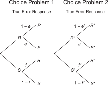
| Figure 1: True and Error Models for two choice problems. In TE4, all four error terms are free; TE2, assumes e = f and e′ = f′; TE1 assumes e = f = e′ = f′ |
Judgment and Decision Making, Vol. 14, No. 5, September 2019, pp. 608-616
Bayesian and frequentist analysis of True and Error modelsMichael H. Birnbaum* |
Birnbaum and Quispe-Torreblanca (2018) presented a frequentist analysis of a family of six True and Error (TE) models for the analysis of two choice problems presented twice to each participant. Lee (2018) performed a Bayesian analysis of the same models, and found very similar parameter estimates and conclusions for the same data. He also discussed some potential differences between Bayesian and frequentist analyses and interpretations for model comparisons. This paper responds to certain points of possible controversy regarding model selection that attempt to take into account the concept of flexibility or complexity of a model. Reasons to question the use of Bayes factors to decide among models differing in fit and complexity are presented. The partially nested inter-relations among the six TE models are represented in a Venn diagram. Another view of model complexity is presented in terms of possible sets of data that could fit a model rather than in terms of possible sets of parameters that do or do not fit a given set of data. It is argued that less complex theories are not necessarily more likely to be true, and when the space of all possible theories is not well-defined, one should be cautious in interpreting calculated posterior probabilities that appear to prove a theory to be true.
Keywords: Error Theory, Hypothesis Testing, Statistics, Bayesian analysis,
Birnbaum and Quispe-Torreblanca (2018) presented software for analysis of True and Error (TE) models (Birnbaum, 2008, 2012, 2013). If we allow that human responses contain random errors according to these models, it ,follows that standard statistical tests might easily lead to systematically wrong conclusions. The following is a classic method to compare rival theories: One theory implies that two situations are behaviorally equivalent (in the sense that the probability of a behavioral response is the same), and the other theory implies that the two situations should produce different responses. If we can reject the hypothesis that the probabilities of response are the same in the two situations, we could reject one theory in favor of the other. A problem with this statistical approach to theory testing can occur if random errors might produce systematic differences in response probabilities. The TEMAP2.R software is intended to provide an alternative, more appropriate method for statistical analysis of two conditions, allowing for a realistic theory of error in responding.
Birnbaum and Quispe-Torreblanca used a variant of the classic Allais paradox to illustrate the error theory and their program. In an Allais paradox, there are two choice problems that should be equivalent, according to Expected Utility (EU) theory. For example, EU theory implies that S = ($48, 0.2; $4, 0.8) is preferred to R = ($96, 0.1; $4, 0.9) if and only if S′= ($96, 0.8; $48, 0.2) is preferred to R′ = ($96, 0.9; $4, 0.1). Other theories, such as Birnbaum’s (2008) models, can imply that people would choose R over S and S′ over R′. This pattern of preferenes is denoted the RS′ pattern, and is considered “paradoxical” because it violates EU theory. The opposite pattern, SR′ is also “paradoxical”. A major question is, are observed violations “real” or are they due to random error?
In the past, the standard statistical test in this situation was the test of correlated proportions. If a number of participants were asked to respond to both questions, or if a single participant was asked on many occasions to respond to both questions, one would compare the frequencies of the SR′ response pattern and the opposite pattern, RS′, and if these were significantly different, one would reject the hypothesis that the probability of response was the same in both conditions. Thousands of research articles used this statistical test. However, we must admit that this statistical test does not really rule out EU, once we realize that random errors might produce inequality of these two types of reversals (Birnbaum & Quispe-Torreblanca, 2018).
Figure 1: True and Error Models for two choice problems. In TE4, all four error terms are free; TE2, assumes e = f and e′ = f′; TE1 assumes e = f = e′ = f′
Birnbaum and Quispe-Torreblanca (2018) noted that the test of correlated proportions in such studies make an unreasonable assumption about errors. If the two choice problems have different rates of error, then it can easily happen that EU theory can hold and the two frequencies of reversal can be unequal; it can also happen that the two frequencies can be equal and yet EU does not hold. Furthermore, according to the TE4 model in Figure 1, the probability of choosing S over R can significantly exceed 1/2 and the probability of choosing S′ over R′ can be significantly less than 1/2 and EU might still hold. These theoretical implications call into question the theoretical conclusions of many previous publications, including some of my own.
Figure 1 diagrams the possible errors in two choice problems. If a person truly prefers R in the first choice problem, she or he might erroneously respond S with probability e. If the person truly prefers S in the first choice problem, he or she might respond R with probability f. In Choice Problem 2, the corresponding errors occur with probabilities e′ and f′, respectively. The model in Figure 1 is denoted TE4 because there are 4 different error rates. A special case of this model, TE2, assumes e = f and e′ = f′, and a further special case, TE1, assumes that e = e′ = f = f′.
In the “true” part of TE theory, it is allowed that a person might have any of four true preference patterns: SS′, SR′, RS′, or RR′, which have probabilities of pSS′, pSR′, pRS′, and pRR′, respectively.
EU theory is a special case of TE in which pSR′ = pRS′ = 0. That is, according to EU, a person never has either of these preference patterns as a “true” set of preferences, but that might respond this way only as a result of one or more errors.
Combining the assumptions about the errors with those about the possible true states, there are six models, TE4, TE2, and TE1, with respective special cases of EU4, EU2, and EU1, which are created by adding the assumption pSR′ = pRS′ = 0.
It might seem that if we allow such an error theory as in Figure 1, then it would be impossible to test EU. Because the four probabilities of true response patterns sum to 1 (pSS′ + pSR′ + pRS′ + pRR′ = 1), they contain 3 degrees of freedom. In TE4 there are four error terms as well (e, f, e′, and f′), meaning that TE4 has 8 parameters to estimate (with 3 + 4 = 7 df). If a study yields data consisting of only four frequencies of the 4 possible response patterns, then the data have only 3 df. Thus, such old-fashioned studies do not allow us to unambiguously test EU, because there remain many possible interpretations of the same data.
However, with a better experimental design, it becomes possible to test not only EU, but also to test the TE models of which EU models are special cases. In particular, to test these models, one needs to replicate each choice problem at least twice for each participant in each experimental session. Replications provide the degrees of freedom required to test the models and test EU. With two choice problems and two replications, there are 16 possible response patterns, with 15 df. Fitting TE4 to the data (consuming 7 df for parameters) leaves 8 df to test the model.
Table 1 shows the frequencies, or counts of the number of times that each of the 16 response patterns was observed in a test of a variant of the Allais paradox (Birnbaum, et al., 2017). (Each choice problem was replicated twice to each participant, embedded in randomized and counterbalanced sequences among many other choice problems in the same session.) For example, 4 of the participants had the RS′ on the first replicate and the RR′ pattern on the second replicate, and 43 participants had the RS′ pattern on both replicates, denoted RS′RS′.
It is assumed that different participants may have different true preference patterns, but they may make different responses on the two replications due to random errors. The errors are assumed to be mutually independent and have probabilities less than 1/2.
Table 1: Frequencies of each Response Pattern
Responses on Replicate 2 Data from Birnbaum, Schmidt, & Schneider (2017), testing a variant of the Allais paradox.
Birnbaum and Quispe-Torreblanca (2018) presented a program, TEMAP2.R, that can be used to perform frequentist statistical tests to fit and test the six models, applied to an appropriate experiment. It is freely available in the online supplement to that paper. The program takes as input the frequency table, as in Table 1. The program estimates parameters to minimize either the standard χ2 index of fit or the G index (sometimes called G2), which is equivalent to a maximum likelihood solution,
| G = 2∑∑Oijln(Oij/Eij), (1) |
where the summation is over the 16 cells, Oij is the observed frequency (count) in Row i and Column j, Eij is the corresponding “expected”, or “predicted” frequency in the cell according to the particular TE model.
The “expected” or “predicted” frequency might better be called a “fitted” frequency because its value is based on the “best-fit” parameter values estimated from the data. It is equal to the number of blocks of data, n, multiplied by the model’s best-fit, calculated probability of showing a given preference pattern.
The G index is similar to χ2 and is also asymptotically Chi-Square distributed. Because EU is a special case of TE in which 2 fewer df are consumed, the difference in fit between the TE model and its corresponding EU special case is asymptotically Chi-Square distributed with 2 df.
TEMAP2.R can be applied with relatively small samples, because it employs Monte Carlo simulation to construct the sampling distribution of the fit statistic, and it uses bootstrapping to estimate confidence intervals on the fitted parameters. Birnbaum and Quispe-Torreblanca (2018) used the data in Table 1 to illustrate their program, method, and the models.
Table 2 shows the computed indices of fit, G, for the six models, fit to the data in Table 1. All of the TE models fit acceptably and all of the EU models can be rejected. The differences in fit between each TE model and its EU special case are in the last row of the table. Each of these differences is Chi-Square distributed with 2 df. TEMAP2.R can simulate the distribution of this test statistic via Monte Carlo in the case of small samples. All are significant, meaning that by frequentist statistical standards, one can reject EU under the assumption of any of these TE models.
One can also compare the differences among the TE models; the difference in fit between the TE4 and TE2 should be Chi-Square distributed with 2 df, and the difference between TE2 and TE1 should be distributed with 1 df. But the differences in this case among TE models are not significant and far too small to argue (on the basis of these data) for one version of TE over another. Comparing the EU models to each other, one might use the differences in fit to argue that the EU models can be significantly improved by allowing more error terms, but such an argument would be dubious because none of the EU models provides an acceptable fit.
The TEMAP2.R program calculates the fitted (“predicted”) values corresponding to Table 1. See for example, Birnbaum and Quispe-Torreblanca (2018, Tables 4 and 5). These predictions showed that each of the TE models gave an excellent approximation to the values in Table 1, whereas all of the EU models systematically failed to reproduce the large frequency (43) for the response pattern, RS′RS′.
Table 2: Indices of fit, G, of TE models to empirical data testing a variant of the Allais paradox.
All solutions fit to 16 frequencies in Table 1. TE4, TE2, and TE1 models have 8, 10, and 11 df, respectively; corresponding EU models have 2 df more; critical value of χ2(df) for df = 2, 8, and 10 for α = 0.05 level of significance = 5.99, 15.51, and 18.31, respectively.
Lee (2018) showed how to apply Bayesian analysis to the TE models to estimate parameters, evaluate models, and compare them. Lee did not question the advantages of the TE models over the previous statistical approach to this issue, but argued that Bayesian methods have advantages over frequentist methods for the analysis of such models. Among the advantages (and also presenting potential issues of debate) is that the Bayesian approach incorporates prior probability distributions over the parameters and uses the new data in accord with Bayes Theorem to revise our beliefs to generate posterior probability distributions of the parameters and posterior probabilities of belief in the models.
For the data in Table 1, the posterior distributions of parameters yielded central values fairly close to the best-fit parameter values obtained by Birnbaum and Quispe-Torreblanca (2018). Figures 2 and 3 of Lee (2018) provide two very informative and excellent depictions of the results of the Bayesian analysis. On the basis of these results, Lee (2018) reached essentially the same major conclusions for the data as found from frequentist methods in Birnbaum and Quispe-Torreblanca (2018); namely, that the EU models do not provide an acceptable representations of the data, and that the TE models can.1
Although I agree with most of the arguments and conclusions in Lee (2018), I have reservations concerning the material in Lee’s (2018, Section 2.5) discussion of model comparisons. I do not find the details of his analysis comparing the six models in this section to be convincing.
Table 3: Posterior Probabilities of 6 models (Lee, 2018).
All solutions based on 16 frequencies in Table 1 and priors of 1/6 for each of the models.
In classical statistical tests, one computes the probability of the data given the null hypothesis, p(Data|H0), and if this probability is less than α, the level of significance, one rejects H0. Table 2 illustrates this frequentist approach for the six models. By these methods, we reject the EU models and we can retain the TE models. In Bayesian analysis, one uses Bayes Theorem to update a prior subjective probability of the hypothesis, given the data, to form a posterior subjective probability, p(H0|Data). Lee (2018) set the prior probabilities of each of the six models to 1/6, and calculated the posterior probabilities for the six models given the data; Lee (2018, Figure 4) found that TE4, TE2, and TE1 to be 0.35, 0.14, and 0.51, with the three EU models having zero posterior probability. These are summarized in Table 3.
Taking ratios of posterior probabilities, Lee (2018) reported a Bayes factor of 3.66 for TE1 over TE2. Although Lee (2018) was careful not to make too much of this particular result, he discussed this type of analysis as a potentially useful standard for model selection. Had the numbers been more extreme, presumably, one might have argued that TE1 is much more likely true than TE2. Lee (2018) states, “Bayes factors measure the evidence the data provide for each model in a way that automatically combines goodness-of-fit with a complete and principled measure of the statistical complexity of the models.”
Such arguments for the Bayes factor for model comparisons among these models strike me as incomplete, and I will set forth in the next section some concerns about Lee’s (2018) approach for comparing these six models. Before I state my concerns, however, I should note that I am not defending nor advocating popular alternative approaches to this same topic, for example, in terms of criteria for goodness of a model that combine fit and number of estimated parameters, such as AIC or BIC. I do not think that either frequentist or Bayesian approach has yet found a way to reduce scientific reasoning to a single computation. Most of my remarks apply to either Bayesian or frequentist approaches to the issue of model selection.
Supposedly, posterior probabilities and Bayes factors, as computed in Lee (2018) indicate that TE1 is more probable than TE2. However, TE1 is a special case of TE2: if TE1 is true, then TE2 is true. By standard probability and set theory, a subset must be less probable or equally probable to any set that includes it. So, I find the result in Lee (2018) that TE1 is more probable than TE2, i.e., that a subset is more probable than a set that includes it, to be problematic. The assignment of prior probabilities of 1/6 to each of the six models implicitly treats the models as if they are mutually exclusive and exhaustive; instead, they are interrelated.
Figure 2 shows the relationships among the models for possible sets of data. Solid lines enclose the TE models; TE1 is a subset of TE2 which is a subset of TE4. The dashed lines represent the EU models; EU1 is a special case of EU2, which is a special case of EU4. In addition, each EU model is a special case of its TE model: EU4 is a special case of TE4, EU2 is a special case of TE2, and EU1 is a special case of TE1. Thus, if EU1 fits the data, than so too do all of the TE models, and if TE4 does not fit the data, than none of the six models can fit the data. There are 10 regions in the diagram. It is possible that data might be compatible with TE2 and not EU4 or that data might be compatible with EU4 and not TE2. The numbers in parentheses in Figure 2 indicate the number of df in the free parameters to be estimated for each model.
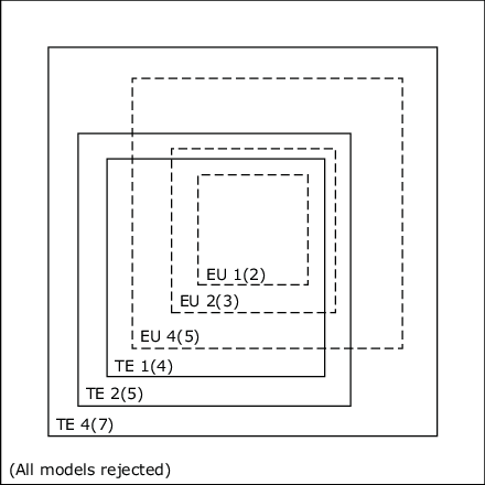
Figure 2: Relationships among the 6 True and Error Models under consideration, with respect to possible patterns of data. Each EU model is a special case of a TE model. There are 10 regions that are mutually exclusive and exhaustive, from EU1 (all TE models acceptable) to all TE models rejected. Numbers in parentheses are the number of free parameters.
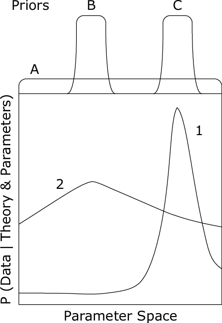
Figure 3: Calculating Bayes factor from priors and likelihood of the data given the model and parameters. Although Model 1 has a better maximum likelihood than Model 2, the Bayes factor favors Model 2 if Priors A or B is used, but favors Model 1 if Prior C is used.
A Bayesian might wish to assign prior probabilities to the 10 regions in Figure 2, including the hypothesis that none of the models is appropriate, and then ask how the data revise those priors to form a posterior distribution over these 10 hypotheses about the situation. I am not sure I know how I would assign prior beliefs over these hypotheses. But I think about complexity of the models in other ways beyond those incorporated in the Bayes factor.
In the Bayes factor, the prior probability distribution, along with the model and the data, combine to inform us how well a model fits, supposedly corrected for how “complex” a model is supposed to be. To compute the Bayes factor for two models, one multiplies the prior times the fit curve and integrates to find the average fit for each model and then computes the ratio. But the prior probability distribution is up to the statistician, making this situation rife for “prior-hacking”, in which a person might influence the conclusions by selecting post hoc a prior distribution to make a favored model or conclusion seem more probable than the disfavored one. With uniform priors, increasing the range of a parameter to include regions of poor fit will tend to “punish” the model with the widened range of parameters.
Computation of the Bayes factor is illustrated in Figure 3 for a hypothetical situation. The abscissa is a simplified representation of a multidimensional parameter space (including parameters for both models) over which the “fit” of the models to the data can be calculated. Note that Model 1 has a better maximum likelihood than the maximum for Model 2. In the figure, the Bayes factor would favor Model 1 if Prior C were applied to Model 1 and Prior B applied to Model 2, but the Bayes factor favors Model 2 if Prior A (which looks “fair” enough) were applied to both models. The argument for the conclusion “supporting” Model 2 in this case would be that because Model 1 is computed to be “more flexible” (because it fits poorly in plausible regions of parameter space under Prior A), Model 1 is less likely to be true, even though it can fit better than Model 2.
Table 4: Percentage of random permutations of data that fit each of the models; “yes” and “no” indicate that the model fit or not to a certain standard.
Based on 70,000 random permutations of data in Table 1.
Some people find the argument “for” Model 2 over Model 1 based on complexity to be unconvincing, and they are troubled that different investigators who started with different priors would reach different conclusions regarding the models from the same data via the Bayes factor. A Bayesian might respond that they should reach different conclusions because their computations reflected different personal beliefs, and Bayes theorem is a method for revising one’s personal beliefs.
A frequentist might respond that journals should not publish personal opinions but only empirical findings. A hacker advocating one model or the other might seek the prior that supports the desired conclusion. If the situation of Figure 3 occurs in a given application, it might be best to report it, rather than simply choose one of the priors and publish the Bayes factors as evidence “for” Model 1 or Model 2.
A Bayesian can argue that any complete model should include not only the structure that leads to the curves for Models 1 and 2 in Figure 3, but also the priors (Lee, 2018). Thus, the definition of “model” should include the prior distribution as part of the model, and so, it is argued, the Bayes factor does indeed evaluate the relative merits of these combined models that include priors. Lee (2018, Section 4.3) acknowledges controversies between frequentists and Bayesians regarding the role of priors in Bayesian inference, arguing that priors are explicit statements of the assumptions of a complete and combined model.
I find this combined approach to model comparisons to be more compelling in cases where there is strong consensus regarding the parameters, established in multiple experiments and contexts. For example, suppose the parameter in Figure 3 represented the measured speed of light in a well-established paradigm. In that case, if prior B represented previous estimates of the speed of light, the argument that Model 2 is better than Model 1 seems strong, since Model 1 requires an odd value for a well-established parameter in order to approximate the data. However, if the parameter represented an individual difference parameter for a previously untested human participant in a previously untested experimental context, I would be dubious of conclusions reached from assumptions regarding previously unknown parameters. I think Lee and I would agree that in such cases, it would be worthwhile to analyze the robustness or dependence of the conclusions regarding the structural models with respect to the prior assumptions on the parameters.
But my concerns extend beyond model selection based on the Bayes factor, where a prior distribution of parameters is assumed, but also to other indices that attempt to combine fit with complexity that do not involve a prior, such as the AIC and BIC, and even to comparisons of overall fit, as measured for example by a correlation coefficients between fitted and obtained values (Birnbaum, 1973, 1974).
In the next section, I discuss another way to think about flexibility of a model, in terms of possible sets of data and possible models instead of in terms of possible sets of parameters and predictions in a limited set of models.
If we imagine a universe of sets of data, how many of them would fall into each of the 10 regions in Figure 2? To address such a question, we need to specify two definitions: First, what is the domain of sets of data? Second, how do we determine that a set of data falls in a region? I will choose two particular operational definitions so that I can illustrate the concepts, but the reader may wish to entertain other definitions.
Define the universe of sets of data as all permutations of the data in Table 1. By permutations, I mean, keep the values in Table 1 and simply rearrange them in the matrix. Next, define “a model fits at level t” if and only if G < t when we choose best-fit parameters in the model for the data to minimize G. (In practice, we can use TEMAP2.R to do these computations.)
Recall that the index of fit, G in Equation 1, depends on two things: The set of observed values, Oij and the calculated “predictions” or “fitted” values, Eij. Because the Oij are permutations of the same values, the index of fit depends on the model’s flexibility in fitting, and not on the values of the numbers, which are fixed in the analysis of this domain.
Sets of simulated data were created by randomly permuting the data in Table 1. Using TEMAP2.R, these simulated data were then fit to all six models. Table 4 shows the percentages of cases (out of 70,000 simulations) that fit each of the six models, for t = 20 and 50. (”yes” means a model fit with G<t). For reference, TE2 and EU4 have 10 df, and the probability that Chi-Square (10 df) exceeds 20 is 0.03.
The row in Table 4 labeled 000000, with “no” in all columns, refers to the case in which all of the TE models do not fit. With t = 20 and 50, 99.65% and 90.70% of the samples failed to fit any TE model. The row labeled 111111 and all “yes” is EU1; all six models fit to the criterion. Row 100000 represents TE4 fitting and none of its special cases. Only 0.2% and 3.6% of the cases fit TE4 and fit none of the other models with G < 20, and G < 50, respectively. Adding up over all ways for TE4 to fit, only 0.35% fit any of the TE models with G < 20, but recall that for the actual data, all three TE models had G < 14. Finally, note that two of the regions of interest, 111000 (all TE and not EU), and the region 100100 (EU4 and not TE2) have roughly equal frequencies of fitting the random permutations.2
Now, suppose we draw in additional theories to Figure 2. These theories may have regions of overlap with the TE models, and they may also overlap the region outside TE4, where datasets reject all TE models. How many theories are there that might be constructed to represent a 4 by 4 table, as in Table 1? I cannot imagine how to count them, nor how to draw all their intersections with the TE models, so I am unable to assign prior probabilities in any meaningful way.
In the game, Mastermind, we know how many theories there are and we know that they are mutually exclusive and exhaustive, so we have an idea how to assign prior probabilities.3 In many cases, however, the space of all possible theories and their mutual intersections is difficult to specify, making proper Bayesian analysis difficult.
Now, suppose we can specify a rival theory, R, to TE4 that partially overlaps the region of TE4 and also occupies space outside it, and suppose there is also a region inside TE4 that falls outside the region of this new theory. Suppose that theory R can achieve a fit with G < 20 to 10% of all permutations of the data, compared to 0.36% for TE4. One might say TE4 is less flexible of a model than R because it can fit a much smaller set of possible outcomes. Perhaps we should grant TE4 a gold star in its favor for being less flexible and still fitting the data, compared to theory R.
However, should we really argue that because TE4 is less flexible that it is also more likely to be true? Are we claiming that a new set of data would be more likely to fall inside the region of TE4 than inside the region of R? Are we claiming that new data are more likely to fall in the region of TE4 that excludes R than in the region of R that excludes TE4? I would prefer to decide such questions empirically rather than by calculations. Empirical evidence that refutes one theory and not the other is more convincing to me than a computation leading one to such conclusions.
Returning again to Lee (2018, Section 2.5), the posterior probabilities say that the union of TE models has a probability of 1 and the EU models have probability 0. I worry about how people with only a course or two in Bayesian statistics would interpret these numbers. Would they conclude that we have proven the TE models to be true? And if true, should not TE fit acceptably in a replication, guaranteed? And if true, should not TE apply in new studies with other stimuli? Of course, such implications are not warranted, but illustrate excess meanings of statements that a theory is “true”. Lee (2018) assumed that one of the six models must be true when he distributed the prior probabilities, and the spectacular failure of EU led to computed certainty for the TE models. I suspect that some people would benefit from education that cautions how to interpret a posterior probability of 1 assigned to an empirical theory.
When students first learn about frequentist hypothesis testing, they are taught that if the probability of the data given the null hypothesis is less than alpha, then one rejects the null hypothesis, but risks a Type I error. It seems natural then that if we “do not reject”, then we should “accept” the null hypothesis, because “accept” is the opposite of “reject”. It is difficult to teach that failure to disprove is not evidence of truth. But people want to draw conclusions from a study, rather than remain undecided. Failure to disprove sounds like proof, but it is not. I teach students to use the words “reject” and “retain”, where “retain” means we simply keep hypotheses around until we have the evidence to reject them.
Hypothesis testing, students eventually learn, cannot prove the truth of the null hypothesis. But Bayesians are willing to compute the probability of the null hypothesis. This is a strong attraction for people who want to know more than what can be rejected, more than what is false; they want to know what we can accept; they want to know what is true.
Consider this theory and its implication, C:
P1: Bread is made of cyanide
P2: All things made of cyanide are good to eat
P3: Fourteen angels love me
C: Bread is good to eat
Our scientist then provides an operational definition of the conclusion, C, that bread is “good to eat” and proceeds to show that the premises of his theory (P1, P2, and P3) “are true” by eating bread. The more times he eats bread and survives, the more “evidence for” his theory he has accumulated, and the more he is convinced that his theory is true. After many trials, he claims he has proven that bread is made of cyanide, that all things made of cyanide are good to eat, and that 14 angels love him.
A skeptic steps in and argues the theory is not proven. Ockham’s razor dictates that premises not used in a deduction should be removed from the argument. Because P3 was not used to deduce C, that bread is good to eat, it can be removed from the system without altering the prediction that was tested. So, by simplicity, P3 can be removed from the system without loss. But does removing P3 make this theory more probable?
It is valid to deduce from the premises that conclusion C follows. So, if the theory is true, then bread is good to eat. However A implies B is not the same as B implies A. A implies B means that if B is false, then A is false. So, if bread is not good to eat, we could reject the theory; but when the conclusion is true we do not know if the premises are true.
The basic ideas that one can “prove” a theory by collecting evidence consistent with it, or make a theory more probable by making it simpler are logical fallacies and should be recognized as such, even when they appear to be justified by what purports to be a Bayesian calculation. The basic human desire to know what is true is seductive: a specious Bayesian argument may seem appealing to those who are mystified by numerical calculations.
How is it, then, that Bayesian calculations can compute answers that seem to defy this logic, such as assigning a probability to H0, if the system is logical? By assumption. If we assume that either H0 or H1 is true, then if we disprove H1, we conclude H0 is true. In some applications (such as coins and cards or a set of mutually exclusive and exhaustive theories), such Bayesian calculations indeed account for all of the possible hypotheses, but in some scientific applications such as model testing for data as in Table 1, the space of alternative hypotheses is not known, so one makes assumptions, and dubious assumptions can lead to dubious conclusions.4
I do not believe that a Bayesian would argue that the TE models can be proven true by posterior probability calculations, but I worry that some others might misunderstand the role and limitations of the assumptions that led to apparent implications that the union of TE models has a calculated posterior probability equal to 1. People might take the values of computed posterior probabilities as if they indicate a theory has been proven true.
Frequentist statistics has been taught in psychology for a century and certain of its misunderstandings and errors of application have been identified in warnings to practitioners. For example, failure to disprove the null hypothesis does not prove the null hypothesis; if a test is “significant” it is not necessarily important or even “real”; significance does not imply that it is likely to be replicated in an exact replication. Reviewers are warned that scientists may run multiple tests, may add studies until a desired result is observed, may select findings, or “p-hack” by other means, so reported p-values may not be what they seem. Some people think that 0.7 is a “high” correlation, that correlation is somehow related to causation, that “causal modeling” does computational magic to allow causal inferences from nonexperimental data, that correlation coefficients can be compared between experiments, that correlation is an appropriate index of fit for model comparisons, or that coefficients in multiple linear regression measure the relative importance of variables. Such misconceptions, and others, are battled by educators and editors.
Just as we have attempted to address these misconceptions of frequentist statistics, with the increased popularity of the Bayesian methods, it becomes important to clarify the limitations of what Bayesian computations can and cannot do. Lee (2018) recognizes the potential controversies regarding priors and states, “Different prior assumptions about plausible response rates will lead to different inferences than the ones we report. This is not surprising, and it is desirable. The priors formalize theoretical assumptions and different theories should, in general, yield different conclusions when applied to the same data.”
Lloyd Humphreys (personal communication, April 15, 1975), stated that “all point null hypotheses (except ESP in a properly designed study) and all models are false.” If so, then frequentist hypothesis testing will inevitably reject null hypotheses and models if given a large enough sample, and no amount of data could convince a Bayesian who accepts such priors to put nonzero posterior probability on H0 or a model. Thus, this reasonable starting assumption means that neither classical hypothesis testing nor Bayesian posterior probabilities can replace other aspects of scientific reasoning that have not yet been reduced to formulas.
I admire both the frequentist and Bayesian statistical developments as intellectual achievements. But I do not think that either approach is yet complete, nor found a way to substitute calculation for design and execution of new experiments that test critical implications of different theories. Students need training to understand the limitations of either statistical approach. Both approaches are vulnerable to misunderstandings, self-deceptions, and reasoning fallacies, some of which are not as well known as others. Some Bayesians are willing to use language that I find troublesome, talking of evidence “for” or in “support” of a theory. I find such language acceptable when the set of all possible theories is finite and delineated, as in cards, coins, Mastermind, or scientific questions where the hypotheses can be divided into mutually exclusive and exhaustive partitions, but not appropriate in an empirical science where the space of alternative hypotheses is not defined.
In summary, I welcome Lee’s (2018) valuable contributions illustrating the Bayesian analysis of TE models including the Bayesian solution for posterior distributions of parameters, evaluations of the posterior predictions of EU model in the context of those of the TE models, and the corresponding identification of loci of failure of the EU model as a description of the data. However, I would urge caution regarding the apparent conclusions that TE1 is more probable than TE2 (even had the Bayes factor been much greater than the calculated value of 3.66), and that the union of TE models have probability 1 of being true. Aside from these concerns, it is worth stating again that the main scientific conclusions from both methods of analysis are in close agreement in this case.
Birnbaum, M. H. (1973). The Devil rides again: Correlation as an index of fit. Psychological Bulletin, 79, 239-242.
Birnbaum, M. H. (1974). Reply to the Devil’s advocates: Don’t confound model testing and measurement. Psychological Bulletin, 81, 854-859.
Birnbaum, M. H. (2008). New paradoxes of risky decision making. Psychological Review, 115, 463-501.
Birnbaum, M. H. (2012). A statistical test of the assumption that repeated choices are independently and identically distributed. Judgment and Decision Making, 7, 97-109.
Birnbaum, M. H. (2013). True-and-error models violate independence and yet they are testable. Judgment and Decision Making, 8, 717-737.
Birnbaum, M. H., Schmidt, U., & Schneider, M. D. (2017). Testing independence conditions in the presence of errors and splitting effects. Journal of Risk and Uncertainty, 54(1), 61-85.
Birnbaum, M. H., & Quispe-Torreblanca, E. G. (2018). TEMAP2.R: True and error model analysis program in R. Judgment and Decision Making, 13(5), 428-440.
Lee, M. D. (2018). Bayesian methods for analyzing true-and-error models. Judgment and Decision Making, 13(6), 622-635.
Vomlel, J. (2004). Bayesian networks in Mastermind. Proceeding of the 7th Czech-Japan Seminar, Awaji Island, Japan. WWW document. https://pdfs.semanticscholar.org/e998/0f631d04094f6fd7a0cbb32e2ca52a5a0301.pdf
Copyright: © 2019. The authors license this article under the terms of the Creative Commons Attribution 3.0 License.
This document was translated from LATEX by HEVEA.