| Figure 1: A Markov model representing transitions in a transitive (TAX) model between true preference states produced by changing the parameter γ. The dataset, Trans 1, was generated with p = q = 0.1 |
Judgment and Decision Making, Vol. 15, No. 1, January, 2020, pp.
MARTER: Markov True and Error model of drifting parametersMichael H. Birnbaum* Lucy Wan# |
This paper describes a theory of the variability of risky choice that describes empirical properties of choice data, including sequential effects and systematic violations of response independence. The Markov True and Error (MARTER) model represents the formation and fluctuation of true preferences produced by stochastic variation of parameters over time, which produces changing true preference patterns. This model includes a probabilistic association between true preferences and overt responses due to random error. Computer programs have been developed to simulate data according to this model, to fit data to the TE model, and to test and analyze violations of iid (independent and identical distributions) that are predicted by the model. Data simulated from MARTER models show properties that are characteristic of real data, including violations of iid similar to those observed in previous empirical research. This paper also illustrates how methods based on analysis of binary response proportions do not and in many cases cannot correctly diagnose what model was used to generate the data. The MARTER model is extremely general and neutral with respect to models of risky decision making. For example, the transitive transfer of attention exchange (TAX) model and intransitive Lexicographic Semiorder (LS) models can both be represented as special cases of MARTER, and they can be tested against each other, even when binary choice proportions cannot discriminate which model was used to simulate the data. Software to simulate data according to this model, and to fit data to this model, to test this model, and to compare special case theories are included or linked to this article.
Keywords: risky decision making, error models, transitivity of preference, Markov model, sequential effects
When a person is presented on separate occasions with the same decision problem, the same person does not always choose the same alternative. This fact, that people are not consistent in their expressed preferences, has led to at least three related problems: First, we would like to understand why a person has reversed preferences. Did the person actually change his or her mind, perhaps by changing the processes or parameters of decision making, or did she or he merely make a random "error", perhaps due to misreading or forgetting the information, errors in aggregating, or errors in remembering or executing the response? If both true changes of preference and random errors are involved, can we separate these sources of variation and estimate their relative contributions?
Second, if we want to construct theories of decision making, it becomes difficult to do so when responses to the same item are not consistent. If a person were perfectly consistent in his or her choices, it would be easier to devise and test theories to describe those choices than if the responses to choice problems contain a lot of variability.
Third, when attempting to test the accuracy of a theory or when comparing rival theories in their descriptive accuracy to data, we perform statistical analyses. However, an improper theory of stochastic variability can lead to systematically wrong inferences: wrong theories can appear to be right and right theories can appear to be wrong, when the wrong statistical model is assumed, so we wish to find a stochastic theory that is descriptive, or at least neutral with respect to the substantive theories that we wish to test and compare.
These problems have been discussed in many previous articles, but solutions are not yet agreed upon (Fechner, 1860; Thurstone, 1927; Luce, 1959, 1997; 2000; Davidson & Marshak, 1959; Becker, DeGroot & Marschak, 1963; Morrison, 1963; Lichtenstein & Slovic, 1971; Loomes, Starmer & Sugden, 1991; Sopher & Gigliotti, 1993; Carbone & Hey, 2000; Hey & Orme, 1994; Harless & Camerer, 1994; Loomes & Sugden, 1998; Butler & Loomes, 2007; Rieskamp, Busemeyer & Mellers, 2006; Tsai & Böckenholt, 2006; Rieskamp, 2008; Wilcox, 2008; Blavatskyy & Pogrebna, 2010; Butler, Isoni & Loomes, 2012; Bayrak & Hey, 2017).
Recent articles on this topic have begun to argue that the variation in choice responses cannot be fully explained by a single process (Birnbaum, 2013; Bayrak, 2018; Bhatia & Loomes, 2017; Cavagnaro & Davis-Stober, 2014; Regenwetter & Davis-Stober, 2018; Regenwetter & Cavagnaro, 2019). The QTest approach (Zwilling, Cavagnaro, Regenwetter, Lim, Fields & Zhang, 2019) allows error to be attributed either to arbitrary random error components or to a mixture of true intentions, but it has not yet provided a method for allowing both sources of variation to be estimated separately from the data. Bhatia and Loomes (2017) explore the effects of random variation in parameters of a decision making model, but note that such variation cannot explain all of the phenomena of choice data, so there must be another source of error.
This article will expand upon an approach based on True and Error (TE) theory (Birnbaum, 2011, 2013, 2019; Birnbaum & Bahra, 2007a, 2012a, 2012b; Birnbaum & Diecidue, 2015; Birnbaum & Gutierrez, 2007; Birnbaum & Schmidt, 2008; Birnbaum, Schmidt & Schneider, 2017; Birnbaum & Quispe-Torreblanca, 2018). This approach does allow separation (and estimations) of the variability due to changes in true preferences and due to random errors. The term True and Error Theory (TET) refers to the general theory that at any given time in a given person there is a coherent set of true preferences, that these true preferences might change over time, and that overt responses may be perturbed by random errors; the term TE model refers to a special case of this theory in which particular simplifying assumptions are imposed; the term TE approach refers to the use of appropriate experimental designs with operational definitions that allow one to test both the TE models and substantive theories via analyses of nested TE models. The TE approach requires analysis of data at a deeper, more detailed level than merely analysis of binary response proportions.1
True changes in preference are said to occur when a person changes the way in which information is evaluated, weighed, and combined. Changes in the value of a parameter, as theorized by Bhatia and Loomes (2017), or changes in the decision making rule, for examples, would produce changes in utility and can thus alter true preferences. Errors are said to occur when a person misreads, misremembers, misaggregates information, or accidentally pushes the wrong response button. Such errors are assumed to be random, but it is not assumed that every choice problem has the same rate of error. These two categories of sources of variation can be disentangled and their contributions separately estimated from the data, if the experiment is properly designed to allow it and if the TE model is empirically descriptive.
The TE approach requires improved experimental designs to properly fit and test TE models. In particular, one must replicate each choice problem within person in each experimental session (block of trials). For example, experimental choice problems can be presented twice in each session, interspersed among many other, similar choice problems. Presentations can be intermixed with filler trials, properly counterbalanced, and presented in randomized orders. A simplifying assumption used in TE models is that preference reversals by the same person in the same brief session to the same item are due to random error. The TE approach requires analysis of detail in the data (including response patterns) rather than analysis only of binary response proportions. Whereas some approaches assume that responses are independently and identically distributed (iid), TE models typically violate independence, and the patterns of violations of iid reveal useful information used in fitting TE models.
TET can be applied in two situations: In group True and Error Theory (gTET), each participant must respond at least twice to each choice problem in at least one session, and there are many participants. TET allows that participants may differ from each other in their true preferences, and TE models assume that preference reversals to the same item in the two replications by the same person in the same session are due to random error.
In individual True and Error Theory (iTET), a single individual is tested in many sessions (blocks of trials); for example, a participant might be asked to participate in an experimental session each day for a number of days, but the key choice problems are presented at least twice in each session (block of trials). The individual is allowed to have different true preferences in different sessions. In models of both iTET and gTET, reversals of preference within a brief period of time by the same person to the same problem are attributed to random errors.2
This article presents an additional component to iTET, in which it is theorized that parameters of a risky decision making process fluctuate within a person according to a Markov process. This addition allows the theory to describe sequential effects that have been empirically observed in previous research but not yet represented within TET. The idea of a Markov process for stochastic parameters was mentioned in Birnbaum (2011) and sketched in Birnbaum (2013, Appendix B). New software has been created for simulation of data according to these models.
Using the simulated data, we will illustrate why it is important to analyze choice data in terms of response patterns rather than merely via binary response proportions. We will generate hypothetical data from either a transitive or intransitive decision making model. We will show that the QTest methods, or any methods that are based on binary choice proportions, fail to correctly distinguish between data generated by a transitive as opposed to an intransitive choice process. We will also show that analyses via TE models correctly diagnose the simulated data.3 We will also show that TE models imply violations of the assumptions that choice responses are independently and identically distributed (iid), and that analysis of response patterns and violations of iid can help identify the stochastic processes used to generate the data.
It is important to distinguish between binary responses (including binary choice proportions) from response patterns (including proportions of response patterns). To illustrate this distinction, consider a test of transitivity of preference among three gambles: A, B, and C. There are three choice problems, AB, BC, and CA. For example, A = ($100, 0.50; $0) represents a risky gamble with a 50% chance to win $100 and otherwise nothing ($0); B = ($92, 0.58; $0); C = ($84, 0.66; $0).
The true preference binary relation is said to be transitive if and only if, for all A, B, and C,
if A ≻ B and B ≻ C, then A ≻ C,
where A ≻ B denotes A is truly preferred to B, where ≻ indicates true preference. Because it is possible that true preferences may change over time, it is helpful to clarify that the statement that true preferences are transitive means that at no time does a person have an intransitive true preference pattern.4 We will describe a model as "transitive," if it implies that true preferences are transitive for all gambles (and all parameters) and a model is "intransitive" if it allows violations of transitivity for any gambles and parameters.
True preferences may change over time and overt responses may contain errors that cause overt response to differ from true preference at the time. So if a single set of observed choice responses from a person violated transitivity, one need not conclude that the person’s true preferences violated transitivity. We distinguish a true preference, represented for example, A ≻ B, from an individual, observed choice response.
We can code responses to choice problems as follows: In Choice Problem AB, let 1 = expressed preference for A over B and 2 = expressed preference for B over A. We can do the same for other choice problems. We could also use this notation to refer to true preferences, but it is important to be clear to distinguish whether the notation refers to true preferences or to observed choice responses.
The term true preference pattern refers to a combination of true preferences in choice problems. For three choice problems, AB, BC, and CA, for example, let 111 represent the following true preferences: A ≻ B, B ≻ C, and C ≻ A (an intransitive pattern), and let 112 = A ≻ B, B ≻ C, and A ≻ C (a transitive pattern). With three binary choice problems, there are eight possible true preference patterns, including two intransitive patterns, 111 and 222, and six transitive patterns, 112, 121, 122, 211, 212, and 221.
The term response pattern refers to a combination of observed responses. We can use the same system of notation to refer to response patterns as to true preference patterns, and it is important to distinguish an observed response pattern of 111 from a true preference pattern of 111. For example, a person with the true preference pattern of 112 might show the observed pattern of 111 by making an error on the CA choice.
If there are multiple blocks of trials (sessions), we can compute proportions of response patterns, P111, P112, P121, ..., P222. Once we know the 8 proportions of patterns, we can always compute the 3 binary response proportions; for example, P(AB)=P111 + P112 + P121 + P122. But we cannot in general reconstruct the 8 pattern proportions from the 3 binary choice proportions.
As noted above, the TE approach requires one to obtain replications within each person and session (block of trials) in order to properly estimate error rates in TE fitting models. For example, one might present each of the three choice problems twice in each session, embedded randomly among many other choice problems, with the positions of the gambles counterbalanced. Note that sessions or blocks of trials are treated as "repetitions" whereas multiple presentations within a brief session are treated as "replications." The term "repetition" is intended to remind us that learning may be involved, so the second repetition of a question is conceptually distinct from the first. In contrast, the term "replication" means that two replications are considered equivalent and could be exchanged without consequence.
If each of three choice problems is presented twice within each session (block of trials), we can define response patterns on all six choice problems. For example, let 111221 indicate that the person showed the intransitive pattern, 111, in one replicate and the transitive pattern, 221, in the other replicate of the same session. With three choice problems presented twice per session, there are 64 possible response patterns per session.
It has sometimes been assumed that choice responses are independently and identically distributed (iid). This assumption simplifies analysis of certain choice models, permits derivation of asymptotic statistical tests, and justifies a focus of attention on binary choice proportions. The assumptions of iid imply simpler properties that are special cases of independence: the probability of a response is stationary (does not change over time), that it is independent of responses to other items, and that it is independent of the sequence of previous responses to the item and other items. With respect to the choice problems studied here, these basic aspects of iid can be written: Stationarity: p(ABt) = p(AB) for all sessions (times), t, Sequential independence: p(ABt|AB1, AB2, ..., ABt−1) = p(AB), and Response independence: p(AB|BC, CA) = p(AB), which should hold for all choice problems.
If choice responses satisfy response independence and stationarity, it means that the probabilities of the 64 possible response patterns (of Section 1.2) contain no more information than is contained in the three binary choice probabilities. If iid holds, then the probability of any response pattern (conjunction of responses) is simply the product of the probabilities of the binary response probabilities. For example, p(111111)=p(AB)2p(BC)2p(CA)2.
In this paper, we will test a special type of sequential independence, which is violated by most MARTER models. We call this property pattern sequence independence, which is the assumption that the response pattern in Session t is independent of the response pattern on Session t−1. We will illustrate how this test can be used to distinguish a special class of MARTER models.
Empirical research shows that choice responses violate iid (Birnbaum & Bahra, 2007b; 2012a; 2012b). Birnbaum (2011, 2012) devised two statistical tests that can be applied with small samples to test sequential independence and response independence. Birnbaum and Bahra (2007b, 2012a, 2012b) found overwhelming evidence of violation of both sequential and response independence by these tests. Birnbaum (2012, 2013) reanalyzed the data of Regenwetter, et al. (2011) and found that even data that had been analyzed under the assumption of iid showed systematic violations of iid.5
TE models do not satisfy iid (they violate response independence, except in special cases), and in fact, they imply violations similar to those reported in several studies: People are more consistent in replications than predicted by random preference models or other models based on iid (Birnbaum, 2011, 2012, 2013; Birnbaum & Bahra, 2007b, 2012a, 2012b; Birnbaum, et al., 2016).
Evidence of sequential dependencies is revealed by Birnbaum’s (2011, 2012, 2013) correlation test; it has been found that there are fewer preference reversals between two blocks of trials that occur closer together in time than between two blocks that occur farther apart in time. This finding suggests that people are not randomly and independently adopting true preferences on each trial or even on each block of trials but instead that people are more consistent in their preference patterns when tested closer together in time.
Birnbaum (2011, p. 680-681) theorized that such results might result from a process in which there are systematic changes of parameters of a descriptive model of risky decision-making over time. Suppose the value of a parameter at time t is likely to persist at time t + 1, and when it does change, the change is not as sudden as it would be if chosen randomly and independently from a distribution. Birnbaum (2013, Appendix B) proposed that this process might be modelled by a Markov process, and that idea is more fully specified here as the MARkov True and ERror (MARTER) theory.
Computer software has been developed that simulates data according to a general MARTER model, and this software permits specification of special cases. This software can be used to simulate data according to particular stochastic process models. The software can even simulate data according to models that do not satisfy assumptions used in previous applications of TE models. Each MARTER model has three parts, or modules.
A MARTER model includes three components (modules), which can be specified separately in the simulation program: First, there is the model of risky decision making (RDM model) that dictates which of two gambles a person will choose in any given choice problem. The RDM model permits different response patterns with different parameters, but the RDM model does not permit all true response patterns. This article will illustrate (in Section 2) two specific rival RDM models: a transitive model (TAX model), and an intransitive model (Lexicographic Semiorders).
The second module is the stochastic representation of how parameters of the RDM model (and therefore true response patterns) can change from time to time. In Section 3, this module will be represented by a Markov process on the possible true response patterns, which correspond to different parameter values in the RDM model.
The third module (discussed in Section 4) is the error model that specifies the stochastic relationships between true preference patterns and observed response patterns. The computer program associated with this paper allows an extremely general specification of errors. It also implements a simple TE model as a special case, in which each choice problem can have a different error rate, and errors are mutually independent.
A key purpose of this article is to show that one can distinguish between data generated by transitive or intransitive processes using TE fitting models as an analytic approach, and that this ability to correctly diagnose the RDM models operates properly even when true states fluctuate via a Markov process. It will also be shown that methods based on binary choice proportions, such as the QTest method (Zwillig, et al., 2019), are unable to distinguish whether the RDM model was transitive or intransitive.
Consider two-branch gambles of the form G = (x, p; y), representing a gamble with a probability of p to win $x and otherwise win $y, where x > y ≥ 0, and 0 < p < 1. Suppose there are three gambles as follows: A = (100, .50; 0), B = (92, .58; 0) and C = (84, .66; 0). We will consider two models that imply preferences and preference patterns among such gambles, once their parameters are specified. One is transitive (it can only imply transitive patterns) and the other intransitive (it can imply intransitive patterns).
Suppose each gamble has a utility. Assume that G ≻ F (a person truly prefers gamble G over gamble F) if and only if U(G) > U(F), where U(G) is the utility of gamble G; all models satisfying this assumption imply that preference is transitive (because the utilities are numbers and > is transitive).
The special TAX model (Birnbaum, 2008) will be used to illustrate a specific transitive model. The special TAX model can be written for two-branch gambles as follows:
| U(G) = |
| (1) |
Where a=pγ(1 − δ/3) and b=(1 − p)γ+pγδ/3, u(x) and u(y) are the utilities of the monetary consequences, x and y, and U(G) is the utility of the gamble. The parameters, γ and δ might differ between individuals, causing different people to have different preferences, and they might change from time to time within a person, producing different true preferences within an individual.
For American undergraduates with modest cash prizes ranging from $0 to $150, it has been found that one can approximate modal choices (group data) with u(x)=xβ, where 0 < β ≤ 1, 0 < δ ≤ 1, and with 0 < γ ≤ 1. For simplicity in this paper, we will fix β = 1 and δ = 1 and explore the preference patterns produced by plausible values of γ. There are four true preference patterns implied when γ = 0.50, 0.55, 0.60, and 65, respectively: 112, 212, 211, and 221.
These same four “true” response patterns are also compatible with expected utility (EU) theory, which is a special case of TAX in which γ =1 and δ = 0, if u(x) = xβ, where β = the exponent of the utility function. The EU model, like cumulative prospect theory (CPT) of Tversky and Kahneman (1992), of which EU is also a special case, however, can not account for systematic violations of coalescing, stochastic dominance, or restricted branch independence (Birnbaum, 2008), so those models have been rejected in favor of TAX based on experiments using other choice problems testing properties besides transitivity.
Thus, this TAX model plays no special role in this analysis of transitivity, but we use TAX here to illustrate a transitive model because it remains compatible with other data that refute other models, and so it remains a viable descriptive model, whereas EU and CPT do not remain viable descriptively. An important point to keep in mind, however, is that none of these transitive models (TAX, CPT, EU, or any other transitive models) could imply true patterns of 111 or 222, no matter what functions or parameters they take on.
If each person had a fixed set of parameters, and if there were no errors, each person would have exactly one of these four true preference patterns as their response pattern, and the same pattern would be observed in every session by the same person. But if the person changes parameters, she or he might have different true preference patterns at different times. In Sections 3 and 4, we will take up how true preferences change from time to time, and how errors can perturb the responses, respectively.
Lexicographic semiorder (LS) models can imply intransitive true response patterns, 111 or 222. In the PH LS model, a person compares two gambles of the form, G = (x, g; 0) and F = (y, f; 0) by first comparing their probabilities to win the higher prize; if the absolute difference, |g − f| > ΔP, where ΔP is the threshold parameter of probability, then the gamble with the higher probability to win is chosen; if the difference in probability does not exceed threshold, choose the gamble with the higher prize.
This model can produce the intransitive cycle, 111; e.g., if ΔP = 0.10 then A = (100, .50; 0) ≻ B = (92, .58; 0) because the difference in probability (.58 − .50 = 0.08 < .10 = ΔP) is not big enough to be decisive and 100 > 92; similarly, B ≻ C = (84, .66; 0) because the probability difference is again too small, but 92 > 84; but C ≻ A because the difference in probability now exceeds threshold (0.66 − 0.50 > 0.10 = ΔP).
This PH lexicographic model can also produce transitive preference patterns, A≻ B ≻ C (112) or C ≻ B ≻ A (221), when ΔP > 0.16 or ΔP < 0.08, respectively. [The priority heuristic model of Brandstaetter, Gigerenzer, and Hertwig (2006) is a variant of this model that implies only the 111 pattern for these stimuli].
Suppose instead a person compares the highest amounts to win first and then probabilities (in the HP LS): that person might have the 222 pattern of intransitive preferences. In HP LS, the difference between the highest prizes, |x – y|, is compared to a cash difference threshold, Δ$, and if this difference does not exceed threshold, the gamble with the higher probability to win is chosen. If $8 < Δ$ < $16, the person would prefer B over A, C over B, and A over C (222). This model can also imply transitive true preference patterns, 112 and 221, for different values of Δ$.
Thus, a person whose behavior can be described by a mixture of PH LS and HP LS might have any of these four true response patterns: 111, 112, 221, or 222.6
Suppose a person’s behavior can be described by the TAX model with different values of γt in different sessions (blocks of trials), where γt is the parameter value in Session t. It seems plausible that a person is likely to keep the same parameters in successive blocks of trials, but when a person changes parameter value, the value drifts to a similar value, rather than jumping randomly to a some different value. Similarly, a person governed by LS models might change parameters from session to session in a similar, gradual fashion. The idea that people remain fairly consistent in their preferences seems plausible, and it agrees with the finding that responses patterns are more similar between sessions closely spaced in time than between sessions farther apart in time (e.g., Birnbaum & Bahra, 2012a, 2012b). We will use the term "gradual" for the theory that parameters may change but tend to remain stable or at least similar from one session to the next.
This theory (1) of gradually drifting parameters can be contrasted with three others: (2) independent change: A person might adopt a different parameters randomly and independently in each session. (3) random preference: A person might randomly and independently adopt a different value of the parameter on each trial. This case combined with other assumptions is sometimes called a "random utility" or "random preference" model. These three stochastic specifications can be contrasted with a fourth possibility, (4) fixed: It is possible that parameters remain constant from session to session, and all of the variability in choice responses to the same item is due to random errors.
In this article, we will develop a fairly general Markov model to describe changing of parameters over time. This general model will be simulated by software that can produce data in each of the categories of parameter variations in the previous paragraph.
Because parameter values correspond to different true preference patterns, we can identify the states of the Markov process either in terms of the parameter values or in terms of the true preference patterns. The general Markov model allows any transition matrix among the true states.
Because there are 8 possible response patterns in this case, the full transition matrix can be represented by an 8 X 8 matrix containing probabilities, pij = the probability of transition from True State i on Session t to True State j on Session t + 1. The Markov model assumes that this transition matrix is the same for all t, and that it is independent of the path, or history of the states, in previous trials.
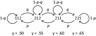
Figure 1: A Markov model representing transitions in a transitive (TAX) model between true preference states produced by changing the parameter γ. The dataset, Trans 1, was generated with p = q = 0.1
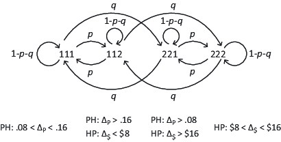
Figure 2: A Markov model representing transitions among preference patterns produced by changing parameters in Lexicographic Semiorders. The dataset, Intrans 1, was generated with p = 0.2 and q = 0.1.
Figure 1 illustrates a transitive stochastic process model in which there are just four true preference patterns that are compatible with the special TAX model (with different values for γ). In this particular stochastic model, a person’s parameter drifts gradually; that is, the person might transition from γ = 0.50 (response pattern 112) to γ = 0.55 (pattern 212) between two successive sessions (blocks of trials), but could not change in successive sessions from γ = 0.50 to γ = 0.65. Many other stochastic models among these four preference patterns are possible. With four states, there are 16 possible transition probabilities with 12 df (because the row sums must add to 1). The model in Figure 1 assumes the stochastic process is summarized by just two parameters, p and q.
Figure 2 illustrates an intransitive stochastic process model in which the four possible states correspond to those implied by different parameters in lexicographic semiorders. Like the model in Figure 1, there are exactly four possible true states, and transitions among them are described by two transition probabilities, but unlike Figure 1, the model in Figure 2 has intransitive patterns, 111 and 222.
The stochastic models in Figures 1 and 2 are both examples of gradual changing parameters, but they differ with respect to the issue of transitivity.
Like the Markov transition matrix, the error matrix is also 8 X 8. It contains entries, eij = the probability given a person is in True State i that the overt response is Pattern j.
The MARTER_sim.htm program is designed so that a user can enter up to 64 error probabilities, representing the conditional probabilities of responding with each response pattern, given each possible true pattern.
The program also allows the option of entering just three error rates, one for each choice problem. One can then push a button to generate all 64 error rates from a TE Model in which each item can have a different rate of error and errors are mutually independent. Thus, the 64 errors (which have 64 − 8 = 56 df, because the entries in each row sum to 1) are reduced by this model to just three parameters (with 3 df) when this version of TE model is implemented.
In this TE model implemented by MARTER_sim.htm, in which the error probabilities are mutually independent, the probability of any conjunction of errors is given by the product of the component errors. For example, if the error rates are e1, e2, and e3 for Choice Problems AB, BC, and CA, then the probability that a person who is in the True State of 112 would show the 112 response pattern is given by: (1 − e1)(1 − e2)(1 − e3) and the probability that the person in the True State of 112 would show the 111 response pattern is given by (1 − e1)(1 − e2)e3.
The theoretical probability in this TE model that a person would show a particular response pattern on two replications within a block, given a True State, is the product of six error terms, similarly constructed. For example, the probability that a person would show the observed pattern 211 and 211 given the true pattern was 111 is e12(1 − e2)2(1 − e3)2. For more information on TE models, see Birnbaum (2013), and for TE models with more complex error assumptions, see Birnbaum and Quispe-Torreblanca (2018).
Although errors in a TE model may be mutually independent, it does not follow that responses will be independent; instead, responses will not satisfy iid, except in special cases, such as when a person has only one true preference pattern (Birnbaum, 2013).
The JavaScript computer program, MARTER_sim.htm, is included in the journal’s supplement to this article. This program is also freely available online at http://psych.fullerton.edu/mbirnbaum/calculators/MARTER\_sim.htm
This program simulates data via the specified MARTER model by starting with a random state, which is set up to transition in one step to one of the permissible states, and then to (stochastically) follow the Markov model among those states according to the transition probabilities specified by the user. (The default values are currently set up to generate data according to a special case of the intransitive model of Figure 4, used to generate the Intrans 2 dataset, described in the next subsection.)
Table 1: Crosstabulation. Frequencies of response patterns in Intrans 2 dataset, simulated from the model in Figure 4.
Total n = 10,000.
To use the program for the first time (with the default values), simply press the button labeled "prepare", then scroll down to the error matrix and press the button labeled "calculate errors by TE"; next, press the button, "row sums errors". Finally, push the button labeled, "many trials with error," which will generate 10,000 true states (stored in the first textarea box), and 20,000 "observed" (simulated) responses containing error (in the second box). The error-filled responses will be selected and focused, so the user can simply copy them (via CTRL & C) and paste them into a program like Excel (CTRL & V), which might require use of the text to columns feature of Excel (they are comma delimited).
The generated data have two replications in each line (session), which are based on the same true state and differ only due to error. This is the standard TE model assumption. There is a button that can be clicked labeled "violation model" that allows the true state to change within a block (within a line), according to the same Markov transition probabilities. This feature allows a user to explore the consequences of this type of violation of the model.
By pasting the data into Excel and using the PivotTable feature, or via other suitable software, one can find the crosstabulation frequencies of each response combination. Table 1 shows the response frequencies for 10,000 simulated sessions, based on the generating model of Figure 4 and parameters used to simulate the Intrans 2 dataset.
A second JavaScript program, iid_sim.htm, available in the online supplement to this article, can be found at the following URL:
http://psych.fullerton.edu/mbirnbaum/calculators/iid\_sim.htm
This program generates data in the same format as that of MARTER_sim.htm, but does so according to the assumption of iid. The data generated by iid_sim.htm can be considered a "control" for comparison with data generated via MARTER models that violate independence.7
Additional instructions for using these programs are included in the Web pages that contain the programs.
The datasets described here were simulated according to seven different generating models; five are based on Markov models of gradual sequential effects, the sixth used a model with pattern sequence independence, and the seventh has binary choice responses satisfying independence and identical distribution (iid).
The dataset, Trans 1, was simulated from the Markov model in Figure 1 with p = q = 0.1, and e1=e2=e3=0.1. The four possible true states correspond to the four possible transitive response patterns: 112, 122, 211, and 221, corresponding to predictions of TAX with the parameter values indicated in Figure 1.
To calculate the steady state (long run) probabilities of being in these states, one can apply basic calculations of a finite Markov chain. A useful on-line Markov calculator for this purpose is available from Fukuda (2004). According to this Markov model, the steady state probabilities of being in these four states are equal; that is, p112 = p212 = p211 = p221 = 0.25. If we had used p = 0.1 and q = 0.2 instead, the steady state probabilities would instead have been 0.07, 0.13, 0.27, and 0.53, respectively.
The dataset, Trans 2, was generated from the Markov model depicted in Figure 3; note that the two possible states (112 and 221) are both transitive and are a subset of the possible patterns of Figure 1. The transition probabilities are given in Figure 3, and e1=e2=e3=0.1. These parameters imply that a person is more likely to remain in the 221 pattern from one block to the next than to remain the 112 pattern between successive blocks.
The steady state probabilities of being in these states (p221 and p112) calculated from the Markov model (Fukuda, 2004) are p221 = 0.67 and p112 = 0.33.
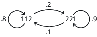
Figure 3: A Markov model that is a special case of the transitive model of Figure 1. This generating model was used to simulate the Trans 2 dataset, but it is also a special case of the intransitive model of Figure 2 in which only the transitive patterns appear.
The dataset, Trans 3, was generated from a transitive model (only transitive response patterns), but it includes patterns not allowed by the model in Figure 1. In particular, the five possible states are 121, 122, 211, 212, and 221. Furthermore, one-step transitions were permitted only between adjacent states in this ordered list (For example, it is not possible to transition from 121 to 221 in one step, but one can reach 221 via the other states). Each transition between adjacent items, in either direction, had a probability of 0.1, except the probability of transition from 221 to 212 was fixed to 0.04, so the probability to stay in state 221 between successive blocks is 0.96. The error rates were e1=e2=e3=0.1. These values were chosen so that the steady state probabilities in the Markov model would be p121 = p122 = p211 = p212 = 0.15 and p221 = 0.40, and therefore, the binary choice proportions would be approximately the same in Trans 3 as in Trans 2. (This generating model is not illustrated in a figure).
The dataset, Intrans 1, was generated from the model in Figure 2 in which p = 0.2, q = 0.1, and e1=e2=e3=0.1. In this model, a person is more likely to transition to a state with only one of the three choices differing than to a state with two differing choice responses; it is not possible to transition from 111 to 222, except via one of the intermediate states. The four states possible in this model (111, 112, 221, 222) are compatible with the lexicographic semiorders, with differing parameters. According to the Markov model, the steady state probabilities of being in each of these four states are equal (i.e., all 0.25).
The dataset, Intrans 2, was generated from the model in Figure 4, in which the possible true patterns are a subset of those in Figure 2: 111, 221, and 222. The probabilities of transitions are shown in Figure 4; e1=e2=e3=0.1. These values were chosen so that the Markov model implies that the three possible states would be equally likely in the long run, and thus, the binary choice proportions would be approximately the same as those of Trans 2 and Trans 3.
The dataset, Intrans 3, was devised to have the same steady state probabilities as Intrans 2 and same error rates, but it differs with respect to the Markov transition matrix. In particular, each row of the transition matrix contained the steady state probabilities as transitions (0.33, 0.33, 0.33); this model thus satisfies pattern sequence independence, as if a person adopts a new set of parameters randomly and independently in each session. (The reader should not assume such a transition model only applies to intransitive cases, as this type of stochastic process could be combined with any of the RDM models.)
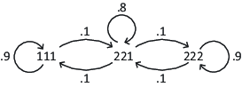
Figure 4: A Markov model, used to simulate Intrans 2 dataset; it is a special case of the intransitive model of Figure 2.
Table 2: Crosstabulation. Frequencies of response patterns in iid 1 dataset, simulated from response independence, and assuming p(AB) = 0.65, p(BC)=0.65,p(CA)=0.35.
Total n = 10,000.
The dataset, iid 1, was generated by the program, iid_sim.htm, which simply calls the random number generator for each response according to its probability, so (if the program’s random number generator works) responses will be independent and identically distributed within and across blocks. To match (approximately) the binary choice proportions of Trans 2, Trans 3, Intrans 2 and Intrans 3, the values 0.65, 0.65, and 0.35 were used for p(AB), p(BC), and p(CA) to simulate the data.
The crosstabulation tables (as in Tables 1 or 2) were analyzed using TE8x8_fit.xlsx, an Excel workbook adapted from Birnbaum (2013) and included in the online supplement to this article. This program uses the solver in Excel to find best-fit solutions to the TE fitting model. The program can be used to minimize either the standard χ2 index of fit or the G index (sometimes called G2), which is equivalent to a maximum likelihood solution. In this paper, we minimized G, defined as
| G = 2∑∑Oijln(Oij/Eij) (2) |
where the summation is over the 64 cells (8 rows by 8 columns), Oij is the observed frequency (count) in the cell, Eij is the "expected", or "predicted" frequency in the cell according to the particular model. The indices, i and j, represent the 8 response patterns for the rows and columns of tables (as in Table 1), respectively; i.e., i= 1, 2, 3, …, 8 correspond to 111, 112, 121, …, 222, respectively.
The 64 "expected" ("predicted") frequencies might better be called "fitted" frequencies because their values are based on the "best-fit" parameter values chosen from the data. Each value is equal to the number of blocks of data, n, multiplied by the model’s calculated probability of showing the given preference pattern.
| Eij = npij (3) |
where pij is the calculated probability of showing this response pattern, given the model and its best-fit parameters. The index G is asymptotically Chi-Square distributed.
The TE models have two components: the probabilities that a person is in each of the possible true states, and the error probabilities relating observed response patterns to underlying true states. The probabilities of the true states are denoted, p111, p112, p121, p122, p211, p212, p221, and p222. Because these 8 terms sum to 1, they have 7 df. In addition, each choice problem is allowed to have a different rate of error, using 3 df. Therefore, the 11 free parameters use 10 df. Because the 64 cell frequencies sum to the number of blocks, there are 63 df in the data. When fitting this TE model with all 11 parameters free, there are 63 − 10 = 53 df remaining to test the model.
Each of the 64 "predicted" or "fitted" frequencies is the sum of 8 terms, representing the probabilities of having each true preference pattern multiplied by the probability of the error pattern that would be required to produce that observed response pattern. For example, the theoretical probability that a person would repeat the 111 pattern on both replications within a block (i.e., 111111) is as follows:
|
where E11 is the calculated, "expected" or ’fitted" frequency of showing this response pattern, 111111. If the person were in the true state of 111, then she could have an observed response pattern of 111111 only if she made no error on all six binary choice problems; however, if she were in the true state of 222, then she would have had to make six errors. There are 64 equations like this one, corresponding to the theoretical frequencies of the 64 observed response patterns, as in Tables 1 and 2.
The specification that preferences are transitive leads to a special case of the TE fitting model in which we fix p111 = p222 = 0, and the probabilities of the other six patterns are free. This stipulation corresponds to the definition of transitivity that at no time is there ever a set of true preferences that are intransitive.
In this paper, we will fit a further special case of the transitive TE model, called transitive4 model, with only 4 transitive patterns, to match the possible true states of the TAX model with varying γ, as in Section 2.1. In this fitting model, p111 = p222 = p121 = p122 = 0, and probabilities of the other four patterns are free, as are the three error rates.
In addition, we fit an intransitive model, intransitive4, which allows the 4 possible patterns under lexicographic semiorders, as in Section 2.2; in this model, p121 = p122 = p211 = p212 = 0, and the probabilities of the other four patterns are free, as are the three error rates.
Each of these special case models, transitive4 and intransitive4, has 4 fewer free parameters than the TE model, so the difference in the indices of the fit between the more general TE model and each special case model is also, in theory, Chi-Square distributed with 4 df. The strategy is to first test the TE fitting model, and then test each of these special case models against the TE model.
In order to keep clear distinctions among a generating model with fixed parameters (used to generate, or simulate a set of data), a particular instance of simulated data produced by that model with fixed parameters, and the fitting model (a model fit to data with certain parameters freely estimated from the data and others fixed), the terms "generated", "dataset", or "fitting" will be appended where needed for clarity. Thus, the Trans 3 dataset, simulated by a transitive generating model with specific parameters might or might not be compatible with the transitive4 fitting model with parameters freely estimated from those data. Fitting models will also be written in Italics, to further remind the reader that certain parameters are fixed and other parameters are estimated from the data.
Table 3 shows the binary choice proportions found in the seven sets of simulated data. Note that although Trans 2, Trans 3, Intrans 2, Intrans 3, and iid 1 were generated from very different models, the resulting binary choice proportions are very nearly the same in these five cases.
Because the binary choice proportions are virtually the same for very different processes, it should be clear that any method of data analysis that relied strictly on binary choice proportions would not be able to correctly diagnose what models were used to generate the data.
The binary choice proportions for five datasets (Trans 2, Trans 3, Intrans 2, Intrans 3, and iid) are nearly identical and they all satisfy both Weak Stochastic Transitivity and the Triangle Inequality. When observed response proportions satisfy these properties, no statistical test is performed in the Regenwetter, et al. (2011) or QTest approach; the fit is considered perfect. In that approach, when binary choice proportions satisfy predictions of a mixture of transitive linear orders, for example, it is argued there is no reason to reject transitivity. An investigator using the that approach in this case, therefore, would incorrectly conclude that data generated from intransitive models (Intrans 2 and Intrans 3) might have arisen from a transitive process. However, by proper analysis of response patterns, we can correctly diagnose the generating models and reject transitivity in these cases, as shown in the next section.
Table 3: Binary choice proportions.
From the crosstabulation frequencies (e.g., as in Tables 1 and 2), one can find the (marginal) binary choice proportions. For example, P(AB) = the sum of row sums for 111, 112, 121, 122, divided by 10,000; one can do the same for columns, and then average the two results.
Table 4: Estimated parameters of the TE model and index of fit (G) to seven sets of simulated data.
Estimated error parameters were all 0.10, rounded to nearest 0,01, except in iid 1, where e1 = 0.34, e2 = 0.35, and e3=0.35. Critical χ2(53) for α=0.05 = 71.0, so TE model fits acceptably in all cases.
In order to fit the simulated data to TE fitting models, we used a slightly modified version of Birnbaum’s (2013) Excel workbook, which uses the solver in Excel to estimate TE parameters to minimize G. This workbook, TE8x8_fit.xlsx, is included as a supplement to this article in the journal’s Website. The program takes as input for each dataset the 8 X 8 crosstabulation frequency matrix, as in Tables 1 or 2, and it finds the best-fit estimates of the error rates for the choice problems and of the probabilities of the 8 true preference patterns.8
Table 4 presents the estimated parameters and fit of the TE model (with all 11 parameters free), applied separately to each of the seven sets of simulated data. In all six sets of data generated by MARTER models, estimated error rates were all 0.10, rounded to the nearest 0.01, closely matching the values used to generate the data. Furthermore, the estimated probabilities of true preference patterns were all within 0.02 of the calculated stable state probabilities of the generating Markov models in all cases.9
The indices of fit of the TE models are all not significant (the critical value of χ2(53) at the 0.05 level of significance is 71.0). Thus, the TE models fit the simulated data acceptably in all seven cases (including iid 1).
Table 5 shows fit indices for the special case fitting models, transitive4 and intransitive4. These fitting models correspond to the particular TAX and LS models stated in Sections 2.1 and 2.2, respectively. They are thus the models that an investigator would naturally want to evaluate for an empirical test between these particular models. For comparison, the first column presents (again) the fit index of TE model with all parameters free (rounded to the nearest integer). It should be no surprise that the Trans 1 data satisfy the transitive4 fitting model, and the Intrans 1 data satisfy the intransitive4 fitting model. It is more noteworthy that Trans 1 data do not satisfy the intransitive4 fitting model, and the Intrans 1 data do not satisfy the transitive4 fitting model. These results show that the TE method of analysis correctly diagnoses data simulated from these two models.
For example, the difference in the G indices for the Intrans 1 data fit to transitive4 compared to the TE fitting model is 4620 − 58 = 4562. This index is theoretically Chi-Squared distributed with 4 df, for which the critical value at the .05 level of significance is 9.5. Of course, with 10,000 blocks of data, it is easy to reach statistical significance; nevertheless, if the same relative frequencies were observed with only 50 blocks of data, the difference would still be more than double that required for significance. (The index of fit is directly proportional to the number of blocks; consequently one can simply divide each G value by 200 and take the difference to make this calculation, 4620/200 − 58/200 = 22.8).
Table 5 also shows indices of fit for transitive4 and intransitive4 fitting models applied to datasets Trans 2, Trans 3, Intrans 2, and Intrans 3. The Trans 2 data, generated from the transitive model in Figure 3, can be fit with acceptable accuracy to both the transitive4 and intransitive4 models. The reason should be clear: the two transitive response patterns (112 and 221) in the data generating model are subsets of the permissible response patterns of both the transitive and intransitive models in Figures 1 and 2, and they are thus common to both fitting models. Thus, the analysis correctly leads to the conclusion that the data in this case provide no reason to reject either the transitive or intransitive models: Both models can be retained.
The Trans 3 data, generated from a transitive model cannot be fit accurately to either the transitive4 or intransitive4 models, and the reason should again be clear: although the response patterns generated are all transitive, they include patterns not allowed by the transitive4 fitting model or the intransitive4 fitting model. This case illustrates that by fitting TE models, the approach has the capability of rejecting one transitive model in favor of another transitive model. In this case, the investigator would correctly reject both of the particular RDM models, in favor of another transitive model.
Table 5 shows that the Intrans 2 and Intrans 3 data violate the transitive4 fitting model, G = 7705 and 7816. Even the transitive model that allows all six transitive response patterns (all patterns except 111 and 222), does not fit appreciably better, G = 7705 and 7815, so we can confidently reject transitivity. But the intransitive4 model fits these datasets, G=68 and 70, so we can retain the Lexicographic Semiorders model of Section 2.2. This analysis via TE fitting models allows us to correctly recognize data that are compatible with an intransitive process and which systematically violate any transitive model.
It is important to note that the binary response proportions of Intrans 2 and Intrans 3 (0.64, 0.64, and 0.37) satisfy both weak stochastic transitivity and the triangle inequality, which some researchers would have taken as evidence "for" or "supporting" transitivity (Appendix B). These examples illustrate how easily one might reach wrong conclusions regarding transitivity from analysis of WST, TI, or other properties of binary response proportions.
The iid 1 data also have approximately the same binary choice proportions as Trans 2, Trans 3, Intrans 2, and Intrans 3. The data of iid 1, generated by iid, satisfy the TE fitting model, G= 47.99. The iid 1 data can be fit acceptably by a TE model in which there is only one true pattern, p221 = 1, and e1 = 0.35, e2 = 0.36, and e3 = 0.35; G = 52.28. When such data are created by an iid random preference model, which is the simplest special case of MARTER model, many interpretations are possible. These data are also compatible with a random utility model consisting of a mixture of linear orders, but it is not possible to identify the probabilities of the true preference patterns in the mixture.
Table 5: Indices of fit of TE models to the simulated data (G). Rows represent the generating models used to simulate the data; Columns represent the models fit to the data with free parameters.
All solutions fit to 64 frequencies. TE, transitive4, and intransitive4 models have 53, 57, and 57 df, respectively; critical value of χ2(57) and χ2(4) at α = 0.05 level of significance = 75.7 and 9.5, respectively.
The five examples with similar binary choice proportions were devised to illustrate four possible cases that are all indistinguishable in QTest or any other method that is based on binary choice proportions, but which can be distinguished with proper analysis of response patterns via TE fitting models: the data might be compatible with both of the (substantive) RDM models (Trans 2), data might refute both RDM models (Trans 3), the data might agree with one model and reject the other (Intrans 2 and Intrans 3), or the data might be non-diagnostic (iid 1).
As we see in the next section, different MARTER models can be diagnosed by different, special-case independence tests that are implied by iid.
Four specific tests of independence are employed here. These can be usefully separated into two categories: response independence and sequential independence. Another distinction is between tests that are appropriate with large samples and those that can be evaluated with small samples.
According to response independence, the probability of any combination (pattern) of responses (as in Table 1) is the product of the constituent binary probabilities. In our tests, the predicted frequency of the response pattern 111111, for example, is calculated from independence as follows:
| E11 = nP(AB)P(BC)P(CA)P′(AB)P′(BC)P′(CA) (4) |
where P(AB), P(BC), and P(CA) are the observed binary response proportions for the AB, BC, and CA choices in the first replicate, respectively, and P′(AB), P′(BC), and P′(CA) are the corresponding binary choice proportions in the second replicate. Each of the other 63 entries in the predicted 8 by 8 table is calculated similarly, as the product of the marginal, binary proportions. One can then calculate G (as in Equation 2) or calculate a standard Chi-Square index of fit. This test of response independence is calculated in the Excel Workbook, TE8x8_fit.xlsx, which can thus be used to compare the fit of response independence to the fit of TE models for the same data.
Table 6: Crosstabulation of Session t (rows) and Session t + 1 (columns) for Dataset Intrans 2
With n = 10,000 sessions, the total is n−1 = 9,999.
Table 7: Crosstabulation of Session t (rows) and Session t + 1 (columns) for dataset Intrans 3.
With n = 10,000 sessions, the total is n−1 = 9,999.
A test of Sequence response Independence could be performed on a different, 8 by 8, crosstabulation matrix, similar to Table 1, but constructed with rows representing the 8 response patterns on one replicate of Session t and the columns representing the 8 response patterns on one replicate of Session t+1. Tables 6 and 7 show this crosstabulation for the first replicate of Intrans 2 and Intrans 3, respectively. If there are n = 10,000 sessions (blocks), then there are n − 1 = 9,999 pairs of successive sessions. These frequencies become the Oij for a test of fit as in Equation 2.
Predicted values (based on independence), Eij, are similar to Equation 4, except E11, for example, now represents the fitted (or "predicted") frequency of the 111 pattern on Session t and 111 on Session t+1, P(AB), P(BC), and P(CA) are the observed binary response proportions for the AB, BC, and CA choices for Session t, and P′(AB), P′(BC), and P′(CA) are the corresponding choice proportions in Session t+1, and n is replaced by n−1, respectively.
A test of Pattern Sequence Independence can also applied to this latter crosstabulation matrix (as in Tables 6 and 7), as follows:
| Eij = (n − 1)P(i, t)P′(j, t+1) (5) |
where Eij is the predicted (fitted) frequency of pattern i on Session t and pattern j on Session t+1, i= 111, 112, 121, …, 222; P(i, t) and P′(j, t+1) are the marginal proportions of response pattern i on Session t and response pattern j on Session t+1 for a given replicate. Given n sessions there are n −1 successive pairs of sessions. Note that if sequence response independence holds, pattern sequence independence follows, but pattern sequence independence does not imply sequence response independence; e.g., P(i, t) may or may not equal P(AB)P(BC)P(CA).
Birnbaum (2012) devised two tests of iid that can be used with small samples, such as one might obtain from individual participants in a small study, as in Regenwetter, et al.’s (2011) replication of Tversky (1969). A slightly revised version of Birnbaum’s (2012) computer program, iid_test.R, which computes these tests (and bootstraps the p-values) is included in this journal’s Website as a supplement to this article.
Both of Birnbaum’s (2012) tests are based on counts of the number of preference reversals (by the same person to the same items) between all possible pairs of repetitions. For example, with 3 choice problems and 2 replications of each problem within each block, there are 6 choice responses per block, so the number of reversals between two blocks can range from 0 (perfect agreement on all six responses) to 6 (six reversals of preferences). If there are 20 blocks of trials, one can choose two blocks 190 different ways, and compute the number of preference reversals between each pair of blocks.
Birnbaum’s (2011, 2012) correlation test computes the correlation coefficient between the mean number of preference reversals between two sessions and the number of intervening sessions (related to the difference in time) between the sessions. According to iid, the number of preference reversals between sessions should be independent of how far apart in time the two sessions are (how many sessions intervene between), but if people can be described by an RDM model with parameters that tend to persist or change gradually, then a positive correlation can occur; i.e., more preference reversals (less similarity) between sessions farther apart than between sessions that occur closer together in time. Birnbaum (2013, Table 11) found that 17 of the 18 participants in Regenwetter, et al. (2011) had positive correlations, 9 of which were significant (p < 0.05).
Birnbaum’s (2012) variance test computes the variance of the number of preference reversals between all pairs of sessions. If responses to related items are governed by an underlying system of true preferences, and if that system differs between sessions, then we expect some pairs of sessions with very few reversals and others with a large number of reversals, so the variance will exceed what is expected by iid. Put another way, the variance of a total will be greater than the sum of the variances when the components of the sum are positively correlated; but if choice problems are independent, then preference reversal on one item will not predict reversal of preference on other items. Birnbaum (2013, Table 11) reported 10 of the 18 participants in Regenwetter, et al. (2011) significantly violated iid by this variance test.
For both test statistics, a bootstrapping procedure is used that randomly permutes each column of data independently. Then the test statistic (variance or correlation) for the original data can be compared to the bootstrapped distribution of the test statistic in randomly permuted data. Birnbaum (2012) showed that the variance test, as bootstrapped by this procedure, gives very similar results to that of the Fischer exact test of response independence for the example cases analyzed.10
Table 8: Tests of response independence and sequence independence.
Critical values of χ2(57) and χ2(49) at α = 0.05 significance = 75.6 and 66.3, respectively. "Resp Ind" = response independence, "Seq Ind" = sequence independence. Small sample tests of iid were fit to 20 subsamples of 20 sessions each. "No. sig var" = number of simulated subjects with significant variances, p < 0.05. "No. sig pos" and "No. sig neg" = number of significant positive and negative correlations, respectively.
Table 8 presents a summary of tests of iid by four procedures. The first column of numbers shows the tests of response independence (Equation 4), applied to the crosstabulation matrices (as in Table 1). All six cases generated by MARTER models with more than one true state systematically violate response independence. Only the dataset of iid 1 (Table 2) satisfies response independence by this test. Even Intrans 3, which has new parameters chosen randomly in each session, violates response independence.
The second column of Table 8 shows the tests of pattern sequence independence (Equation 5), applied to the crosstabulations between response patterns on Block t and on Block t+1, as in Tables 6 and 7. Note that the first five datasets generated by MARTER models have significant violations of this property, whereas Intrans 3 and iid 1 satisfy this property.
To compare Intrans 2 and 3, examine Tables 6 and 7: In Table 6 responses are highly consistent between successive sessions (note the large frequencies on the diagonal for Patterns 111, 221, and 222), but in Table 7 (Intrans 3), response patterns are as likely to change from one session to the next as to stay the same (e.g., in the first row of Table 7, note the large frequencies of transitions to 221 and 222 following 111).
In order to understand what MARTER models imply for experiments in which each participant only serves in a small number of repetitions, we simulated data of hypothetical individuals, as if they had performed only 20 sessions (blocks). We extracted 20 successive blocks of data to generate a "subject," and then did this 20 times in each dataset. Keep in mind that these "subjects" are clones, simulated from of the same MARTER model with the same parameters. Each "subject" (with 20 blocks) was analyzed separately by the program iid_test.R.
The last three columns in Table 8 show results for 20 simulated "subjects" with 20 blocks each in each dataset. The numbers in the last 3 columns represent the number of simulated "subjects" who had "significant" variances, positive, and negative correlation coefficients. Because there were 20 significance tests at the 0.05 level, one would expect a (mean) tally of 1 in each cell of the variance test, if iid held in the data. Also assuming iid, one would expect an equal number of significant positive and negative correlations, and the sum of both positive and negative significant correlations would also be expected to equal (on average) 1 in each dataset.
Instead, Table 8 shows that every dataset generated by a gradual MARTER model with a mixture of true preference patterns has an excessive number of "significant" variance tests (from 7 to 17 out of 20), that there are more significant positive correlations than negative ones (30 versus 2), and that the total number of significant correlations is excessive (32 out of 100). These results indicate that MARTER models generate the kinds of violations reported by Birnbaum (2012, 2013) in his reanalyses of the small-sample data of Regenwetter, et al. (2011).
In contrast, the "control" condition of iid 1 showed no significant deviations by any of the tests of iid. Intrans 3 had significant violations in all 20 cases of the variance test (response independence), but only two "significant" correlations by the correlation test. Because the Intrans 3 dataset was generated by a process that creates independence between sessions, it should not produce violations of the correlation test. But it is also a TE model with a mixture of true states, so it violates response independence, which are revealed via the variance test.
The distinction between the generating models of Intrans 2 and Intrans 3 illustrates the distinction between Birnbaum’s (2012) correlation and variance tests. To illustrate further, we selected an additional 100 simulated "subjects" with 20 sessions (20 blocks) from each of Intrans 2 and Intrans 3. In Intrans 2, there were 69 and 40 significant violations of iid by the variance and correlation tests, (39 of 40 significant correlations were positive). In Intrans 3, there were 99 significant variance tests and only only 5 significant correlations (as expected when p < 0.05). Intrans 2 has fewer violations by the variance test because of the sequential effects in which a person is likely to remain in the same true state in a short study, leading to lower variance of true states compared to Intrans 3, in which a person jumps states randomly. But Intrans 3 has only a chance level of significant correlations because it has no sequential dependence from block to block, so it should theoretically not produce significant correlations except by chance.
Even though the first six MARTER datasets were constructed by a process that violates iid, not all individual "subjects" (subsamples of 20 blocks) showed significant deviations by these small-sample tests of Birnbaum (2012). For example, in the Trans 1 condition, only 7 and 5 of the 20 simulated subjects with 20 blocks of data showed significant violations of iid by variance and correlation tests, respectively.11
In sum, the MARTER models generate data that violate iid, and the tests proposed to test iid correctly detect those violations, but when we use only small subsamples of the data, as in the small samples obtained in studies with individuals, not all tests are significant.12
The violations of response independence, evident in Table 1 (but not in Table 2 for iid 1) and measured by the index in the first column of Table 8, can be described by the TE model. But the violations of pattern sequence independence, evident in Table 6 for Intrans 2 (but not in Table 7 for Intrans 3) and tested in the second column of Table 8, require theory beyond the basic TE model for their description. That is, the TE model is compatible with such violations, but it does not predict them without additional theory. That additional theory in MARTER is the Markov model of changing parameters.
The msm package in R by Jackson (2011, 2019) can be used to fit Markov models to empirical data. To fit our simulated data, we applied msm using a latent Markov model with "misclassification" ("error" in MARTER). In msm each datum must be linked to a time (because the probability of a transition is a function of time interval). We assigned successive integers for the times of successive sessions (blocks), but we added 0.001 to the second replicate in each block. The response patterns, 111, 112, 121, ..., 222, were re-coded with successive integers from 1 to 8, respectively, representing the 8 states. We treated each dataset as if from a different, single participant, so there were 20,000 lines of data for each case.
There are 64 transition intensities and 64 error rates to estimate from the data. However, because the sum of entries in each row must sum to 1 in each of these matrices, there are 128−16 = 112 degrees of freedom in the parameters to be estimated by msm from the data. For initial estimates of the transition intensity matrix, we set all off-diagonal entries to 0.125 and all off-diagonal entries of the error matrix to 0.05. These are not optimal starting values, but the program did a good job of recovering the generating models.13
Table 9: Estimated Markov Transition Matrix from Session t (rows) to Session t + 1 (columns) for dataset Trans 1
Fit to 20,000 response patterns via msm. Probabilities of transitions to other patterns were estimated to be 0, rounded to the nearest 0.0001.
The msm program yields estimates of the 8 by 8, one-step transition matrix and of the 8 by 8 error matrix. For Trans 1, all 32 transition probabilities to states other than 112, 212, 211, and 221 were estimated to be zero, rounded to the nearest 0.0001. That is, the msm program correctly identified the set of true states. The estimated transition probabilities among these four states are shown in Table 9. In all cases, the estimated values, rounded to the nearest 0.01, are within 0.01 of the values used in the generating model to simulate the data (Figure 1).
The estimated error matrix is also 8 by 8; however, error probabilities from states that cannot be reached are moot (they play no role in fitting the data), so the relevant numbers in Trans 1 are the 4 True States by 8 Observed States matrix. All of these 32 estimated error rates were also within 0.01 of the values used in the generating model.
Results for the other four datasets generated from MARTER models were similar. All estimated transition probabilities to states that could not reached in the generating model were correctly estimated to be near zero. The largest deviation in these five datasets was 0.03. All estimated transition probabilities among states possible in the generating model were close to the values used in the generating models, with a largest deviation of 0.01. Finally, all estimated error rates for states possible in the model were close to the values used in the generating model, with the largest deviation being 0.01. In sum, msm was able to come quite close in estimating the parameters used to simulate the data.
When fitting the iid 1 data by msm in the same way, the estimated transition probabilities were all 1.00 from any state to 221, except for the transition from 111 to 221, estimated to be 0.99. The estimated error rates for responding 111, 112, 121, 122, 211, 212, 221, and 222, given the true state of 221 were 0.08, 0.05, 0.14, 0.08, 0.15, 0.08, 0.28, and 0.14, respectively. Thus, msm correctly diagnosed the iid data as a case with no systematic sequential transitions among states, since there was just one true state.
The program msm also correctly detected the distinction between Intrans 2 and Intrans 3, which are not distinguished by the TE fitting models (Table 4). The transition probabilities estimated by msm in Intrans 3 were all approximately 1/3 for any transition among the three possible states (largest deviation = 0.02); thus, msm correctly indicated that the data of Intrans 3 fit a process in which the true preference pattern on one session is independent of that on the previous session.
In this paper, we have addressed five related topics: (1) We have developed the MARTER theory of stochastic effects in choice tasks and have presented new software that simulates data according to this theory. (2) We have shown that the MARTER models can create systematic violations of iid, that these violations resemble those previously reported in the literature, and we have proposed specific tests of iid that distinguish different stochastic processes. (3) We have shown that software previously developed to fit TE models and Markov models can be used to correctly diagnose data simulated by MARTER models. (4) Our examples illustrate how the MARTER approach can be used to test a critical property like transitivity. TE and Markov analyses correctly diagnosed the simulated data, whereas (5) Methods based on binary choice proportions (Appendix B) are not able to distinguish whether a transitive or intransitive model had been used to generate the data.
In the next five sub-sections we discuss these themes and in the sixth sub-section, we describe wider applications and extensions of MARTER models and appropriate methods of data analysis.
MARTER models are special cases of a general theory in which one specifies three modules: (1) a "substantive" model of the underlying task. In the cases illustrated here, the substantive models are rival models of risky decision making that allow different true preference patterns under variation of their parameters. (2) A Markov process is used to describe how parameters change from time to time. We think that people tend to be consistent in the short run, and may change over time gradually, as in the first five MARTER models illustrated here; such models can be contrasted with random preference models in which responses are represented as an independent random sample from the set of possible true preferences on each trial (iid 1) or in each session (Intrans 3). (3) An error model is used to represent the relationship between true preference patterns and overt response patterns. In the TE model we used to represent errors, errors are mutually independent.
As we have shown here, MARTER models are testable descriptive models that can reproduce phenomena observed in empirical studies. They allow one to describe variability of response, violations of iid, and sequential effects observed in previous research, such as those reported in Birnbaum and Bahra (2007b, 2012a, 2012b), Birnbaum, et al. (2016, Appendix A), and other studies.
Aside from its role as a descriptive theory, MARTER serves as a framework for statistical analysis of empirical data, in which the investigator wants to evaluate rival substantive theories that can be stated as special cases. We consider the data-analytic framework (of fitting and testing nested MARTER models) to be more appropriate than the use of "off the shelf" statistical methods derived from assumptions of iid.
Birnbaum and Quispe-Torreblanca (2018) showed that the classic test of correlated proportions, which had been the standard statistical test of the Allais paradox for five decades, can easily reach wrong conclusions if the error rates for different choice problems in TE models are not equal. A reanalysis of empirical data using TE models found that the paradoxical behavior is indeed real and not merely an artifact of an inappropriate assumption concerning the error rates.
In the simulations analyzed here, transitive and intransitive models were specified and tested as special cases of MARTER. Many other rival theories of choice and judgment could be evaluated and compared as special cases. It is precisely because this approach does not force properties such as transitivity that it can be used as a relatively neutral statistical judge for the comparison of rival models. MARTER can thus be viewed as analogous to Analysis of Variance.
Our simulations show that MARTER models produce violations of iid that resemble results observed in empirical data.
The clearest evidence that iid is not empirically descriptive was reported by Birnbaum and Bahra (2007b, 2012b). In tests of transitivity of preferences among gambles, they found a number of participants who had perfect reversals of preference (on 20 out of 20 choice problems) between sessions, similar to the reversals implied by the MARTER models specified here. Many others had 18 or 19 reversals between sessions. But the same people had very few reversals between replications within the same session.
In this paper, we defined and tested specific independence properties including response independence and pattern sequence independence. The TE model, by itself, implies violations of response independence when there are multiple true patterns in a mixture. By adding the Markov model to the TE model, the MARTER model can fit both types of violations of iid reported. Pattern sequence independence is violated by MARTER models in which people change parameters gradually, and it is satisfied only in special (and we think, unrealistic) cases such as Intrans 3, where parameters are randomly and independently selected in each new session.
To simulate violations of iid that resemble previous findings, we used MARTER models in which parameters change gradually. We found that the MARTER models can produce positive correlations between the number of preference reversals and the gap between sessions, as found in Birnbaum’s (2012) reanalysis of Regenwetter, et al. (2011) data and in other datasets. But even though the small subsamples of simulated data were all drawn from the same process (all clones), not all small sample tests were significant.
Our analyses of simulated data via TE fitting models illustrate that the Markov model of sequential effects for changing parameters combines seamlessly with the TE fitting model for data analysis. In every case we have examined so far, estimated probabilities of the response patterns in the TE fitting model solution matched very closely the stable state probabilities of the Markov generating model used to create the data.
In every case we have examined so far, states not possible in the MARTER generating model were correctly estimated in both the TE fitting model (via TE8x8_fit.xlsx) and in the Markov fitting model (via msm) to have near-zero probability; therefore, these methods of analysis appropriately distinguished RDM models that allow different true response patterns.
Data generated by the transitive TAX model were correctly diagnosed as transitive and consistent with that model, data generated by intransitive LS models were correctly identified as intransitive and consistent with LS, data generated by a process that might have been governed by either model were correctly diagnosed as compatible with either model, and data generated by a model violating both models under consideration were also correctly identified as such. Thus, the use of TE fitting models correctly identified the RDM models used to generate the data. The success of the TE fitting models in diagnosing the simulated data is noteworthy because other approaches fail to correctly diagnose these data.
Luce (1997) reviewed several unsolved problems of mathematical psychology, including an issue that Regenwetter, et al. (2010) called "Luce’s challenge". In particular, Luce noted the tensions among deterministic, axiomatic algebraic theories (of the structure of such problems as risky decision making), stochastic models of choice, and statistical analysis of numerical data. Algebraic models are stated in the form of deterministic qualitative axioms; it was not clear how to test such axioms empirically in the presence of error. We think Luce sought a fundamental, qualitative, axiomatic theory that would include these separate systems in a single coherent structure.
Regenwetter, et al. (2010, 2011) reformulated these unsolved problems as a program to recast deterministic axioms as probabilistic models and to develop appropriate statistical methodology to test these probabilistic restatements of deterministic axioms. They called this program "Luce’s challenge". Their method advocates testing the triangle inequalities or more generally, testing whether a set of binary response proportions are compatible with implications of a mixture of (transitive) linear orders using binary response proportions. But as shown here (and see Appendix B), this approach cannot be relied upon to correctly identify whether data were generated from a transitive or intransitive model.
Regenwetter, et al. asserted that their approach was "the currently most complete solution to the [Luce’s] challenge in the case of transitivity of binary preference." But that approach cannot distinguish whether the generating model was transitive or intransitive in the cases we simulated.
We analysed five cases with virtually identical binary response proportions that perfectly satisfied both weak stochastic transitivity and the triangle inequality. The mixture of (transitive) linear orders fits "perfectly" in all five of these cases. Although the Regenwetter, et al. (2011) approach would declare all five cases to be perfect fits to a mixture of transitive orders, we know that Intrans 2 and Intrans 3 were generated from an intransitive model and we found that the TE fitting model correctly identifies these cases as intransitive.
Therefore, we do not agree that that the Regenwetter, et al. approach is the "currently most complete" solution to Luce’s challenge in the case of transitivity, because it cannot be trusted to correctly identify whether data were generated from transitive or intransitive models. The conclusions of Regenwetter, et al. (2011) that transitivity of preference was acceptable for their 18 participants should therefore be taken with a grain of salt, even though this conclusion is compatible with other recent findings that employed better methods of data analysis. A brief review of recent research in which incidence of transitive and intransitive behavior can be estimated is included in Appendix C.
A major factor limiting the QTest approach is that binary choice proportions do not contain enough information in the data to reliably distinguish cases where transitivity is or is not satisfied. Although there are extreme cases where binary choice proportions might lead to correct rejections of transitivity (e.g., as in Appendix B, when TI can be rejected), there are many cases, as illustrated here, where binary choice proportions simply cannot correctly assess transitivity. And even when the method leads to rejection of transitivity, it is not capable of estimating the incidence of intransitive patterns.
The assumption of iid in the QTest method is used in the statistical tests of properties such as the TI, so one would certainly prefer that such tests ought to be based on more realistic statistical assumptions. But we consider the statistical assumption of iid for significance testing to be a less serious problem than the conceptual assumption of iid to justify analysis of binary response proportions without checking response patterns.
It is the violations of iid (e.g., via response patterns as in Table 1) that inform us that binary choice proportions are not the whole story, and it is the information in those violations of iid that allow the TE fitting model to correctly reject transitivity, even in cases where the TI fits perfectly and significance testing is moot.
It is the response patterns corresponding to violations of iid that not only permit TE analysis to distinguish data constructed from transitive or intransitive models but also to estimate the proportion of participants who have true intransitive patterns or the proportion of sessions where an individual has true intransitive preferences. So, rather than ignore violations of iid, to hope they don’t matter, or to try to "avoid" them by experimental procedures, we should welcome and analyze them because of the information they provide.
It is a major problem that methods based on binary proportions can achieve perfect fit for the wrong theory and could thus lead to wrong conclusions even with population data. One might argue that if a mixture model of (transitive) linear orders can "mimic" a truly intransitive process with respect to binary response proportions, we might as well adopt such a model for its ability to "mimic" data. However, we disagree. Rather than blame (or praise) the models, as if they intended to (succeeded) fool us, we should simply admit that binary choice proportions simply don’t distinguish the models. We need to look deeper in the data, such as the response patterns.
Regenwetter, et al. (2010, 2011) disparaged what they called "pattern counting," apparently because certain early attempts to analyze the frequencies of response patterns lacked theoretical rigor to separate errors from true preferences. However, once we can model them, frequencies of response patterns contain information about binary choice proportions. From the perspective of response patterns, one can view models of binary proportions as under-identified and over-simplified special cases. Any model of response patterns makes predictions for the binary choice proportions.
The TE models provide for at least two statistical tests: First, one can test a TE model. Second, within that model, one can test a substantive property as a special case of that model. So, rather than assume that iid holds, that errors are of a certain arbitrary magnitude, or that all choice problems have the same error rate, one can test these assumptions in the MARTER framework. An example comparing six models (with three nested TE models that impose various assumptions concerning errors and in each of which EU is a special case)is presented in Birnbaum and Quispe-Torreblanca (2018) and discussed further from a Bayesian perspective in Lee (2019) and Birnbaum (2019).
In the TE fitting model used here, it is assumed that the two replications within each session are governed by the same underlying true preferences. Suppose, however, that within sessions, people might change true preferences. Would we be able to detect this violation of the modelling assumption? The MARTER_sim.htm program allows one to explore this issue: By clicking a button marked "Violation model" in the program, one can generate data by a model in which the second, so-called "replication" is actually based on true states that reflect one step in the Markov process (the same Markov transitions that apply between sessions is applied within the session between two "replications").
We simulated data according to the six MARTER models used here, except with this "Violation model" button clicked. In all six cases, the TE fitting program correctly detected that the TE model does not fit. Instead of G values less than the critical value of 71 (α = 0.05 significance level), as found in Table 4, the six G values for the violation model ranged from 277 to 8681, all significant. Interestingly, even though the TE model did not fit, it gave estimates near zero for response patterns that were zero in the generating model; therefore, the TE fitting model still correctly distinguished transitive from intransitive generating models. We are currently exploring the ability of the TE fitting model to detect violations, and the robustness of parameter estimation. Our initial simulations show that for the six cases studied here, one would have detected the violations and yet the conclusions regarding transitivity would nevertheless have been correct.
A reviewer asked how MARTER models might be applied in a multi-day experimental design, such as in Birnbaum and Bahra (2007b, 2012b). In those studies, participants served in many sessions, with two replications per session; they then returned one week later to serve again in a number of sessions with replications. Sessions were separated by intervening judgment tasks. There were three, 5 by 5 interlocked tests of transitivity, each with all 10 pairwise comparisons among the five stimuli. That study found extreme violations of iid, which were observed in several studies despite changes in experimental procedures.
The nature of violations of iid observed was clearest for a subject whose data are presented in Birnbaum and Bahra (2012b, Table 2). By the seventh session of the first day, all 60 pairwise judgments (3 designs by 10 pairwise choices among the 5 stimuli by 2 replications) were perfectly consistent with transitive preference orders, ABCDE, FGHIJ, and KLMNO. That same subject had similar preferences in the first session of second week, but by the 8th session of that week, all 60 responses were exactly opposite those of the 7th session of the first week. Such complete reversals of preference are possible (and predicted) under MARTER models. The reviwer’s question of how to model such data can be rephrased as a question of how to measure the effect of time between sessions that might occur on the same day or different days.
In a continuous time Markov model as implemented in Jackson’s (2019) msm, the probability of a transition between states is assumed to be the same in any equal interval of time. One can ask if the probability of a transition between two successive sessions would be the same if they occur on the same day or on different days. This issue seems to be an empirical question that could be analyzed via MARTER models. One could fit the data using multiple scales of the time variable, and then choose that scaling of time that provides the best fit. In principle, the Birnbaum and Bahra (2007b, 2012b) design could be fit by a MARTER model, but in practice one would need a greater number of sessions and days to be able to properly estimate and test such MARTER models.
What would one need to do to properly investigate this family of data-hungry models? Such an experiment would be a long one, but not impossible to do. The requirements exceed what has been done as of yet to our knowledge, but are not excessive compared to certain studies in cognitive psychology. Such a study might be designed to test the hypothesis that specific educational interventions might produce systematic violations of the Markov assumption. Imagine a study in which participants are randomly assigned to one of two groups in a five month experiment. In both groups, students return to the lab for one hour once every week and serve each time in 10 sessions with 2 replications in each session. In one hour per week for 20 weeks, each individual in each group could generate sufficient data to fit and test MARTER models.
In the treatment group, participants would be enrolled in a course on Decision Making, in which students learn about normative and descriptive decision making models, whereas the control group would receive no such specialized education (beyond the regular curriculum). It seems plausible that in the treatment group, there might occur learning– insight, "ah ha" moments, when a person suddenly changes to a different (and perhaps more normative) way of making decisions. One could search for such evidence by fitting MARTER models in order to show that the estimated transition matrices before and after the intervention event are different. The null hypothesis, which might be more plausible in the control group, is that the transition matrix remains the same throughout.
Because MARTER models allow one to estimate error rates (as well as the probabilities of the true preference patterns), they seem well suited as fitting models for the investigation of such questions as follows: Are error rates higher when participants have less experience, when there is time pressure, when stimuli are closer in value, when alcohol has been consumed, when there is more information to process, or when visual or auditory displays are more complex? Rates of error appear to vary strongly among individuals (e.g., Birnbaum & Gutierrez, 2007); can one predict a person’s error rate from tests of personality, IQ, or other individual differences measures? TET and MARTER allow one to measure and evaluate such questions but these theories do not constrain the answers to such empirical questions. Rival models, such as those considered in Rieskamp, et al. (2006), Marley and Regenwetter (2016), Busemeyer and Townsend (1993) or Birnbaum and Jou (1990) might be evaluated by testing them as special cases of MARTER.
As a simple example, Case V of Thurstone (1927) can be written as a special case of MARTER in which there is only one true, transitive preference ordering, and error rates are inversely related to the separation of the stimuli via the cumulative standard normal distribution. One could first apply the TE fitting model and ask if one true preference pattern has estimated probability of 1 and if the estimated error rates in the full model satisfy the implications of Case V; second, one can also build in the Case V constraints as a special case of MARTER.
Do any of the datasets analyzed here fit Thurstone Case V? The answer is that only the iid 1 data are compatible with one true preference order, so Thurstone Case V would be rejected for the other datasets, based on Table 4. In Table 4, we see that the estimated errors of iid 1, which are approximately equal to each other, do not satisfy Thurstone Case V because if e1=0.34 and e2=0.35, then Case V implies e3 should have been 0.21, contrary to the solution in Table 4. When we fit the special case of TE (fixing p221 =1 and constraining e3 to Case V and the others freely estimated)14), the best-fit TE solution of iid 1 to Thurstone Case V yields G = 586.9, so these particular data (Table 2) are not compatible with Thurstone’s Case V, even though they satisfy a TE fitting model with p221 =1.15
Table 10: Available software used in this study
All software listed here, together with example data files, are available from the supplement to this article in the journal’s website.
How can one combine MARTER models across individuals? Given extensive data for each of a number of individuals, one might fit a MARTER model to each participant separately. However, one might also specify a hierarchical set of models to represent individual differences. We think it a reasonable starting hypothesis that all participants might have the same underlying RDM model (the same set of possible true states) but participants differ in the Markov processes by which their parameters change from time to time and in their error rates. It would be interesting if data require rejection of this model in favor of a more general one in which different people are governed by different RDM models as well as in the parameters and transitions among parameters in the model.
The main software used in this project is listed in Table 10. The simulation programs are open source, free software that should be useful to help researchers understand these models. The software for analysis under the TE fitting model and for testing iid is also free and open source. Two items not listed in Table 10 are the msm software by Jackson (2019), for fitting Markov models, and a Python program used to automate the selection of subsamples of data (to simulate individual "subjects") and set up the files for testing iid. The Python software, along with a guide to using it, is also included in the journal’s online supplement to this article.
A reviewer requested clarification of terms used here, "theory", "model", and "approach." A theory is a set of statements proposed to explain certain observable phenomena, that satisfies five philosophical criteria for scientific explanation: (1) deductive: One can deduce the phenomena to be explained from the theory, (2) meaningful: one can specify operations of measurement and empirical tests that could in principle falsify the theory, (3) predictive: In principle, one could have predicted the phenomena, given the explanation, (4) causal: In principle, one could manipulate the phenomena to be explained, given the explanation, and (5) general: The premises can be used to explain other phenomena.
A model is a special case of a theory in which additional assumptions are made that make the theory easier to work with in practice; the simplifying assumptions are made to facilitate estimation of parameters, for example. It is often believed that these additional modelling assumptions are not actually true but reasonable approximations, so it is sometimes said, "all models are wrong".
For example, consider two theories: that the Earth is round (convex) or flat, to explain observable phenomena such as apparent positions of the stars viewed at different times and places on Earth. In order to estimate the size of the Earth within the "round earth" theory, Eratosthenes adopted simplifying assumptions: He assumed the earth is a perfect sphere and that the sun is so far from the earth that light rays from the sun are essentially parallel as seen from anywhere on Earth. The existence of mountains, valleys, and tides were already known to contradict the perfect sphere, and the idea of parallel light rays was understood to be an approximation. But by using these modelling assumptions, he was able to compute a reasonable estimate of the Earth’s diameter based on only two observations of the angles of sunlight relative to plumb lines at two points on Earth, separated by a measured distance.
In sum, a model is a special case of a theory that adds additional assumptions, which are often recognized as only approximations. Any model therefore also qualifies as a theory, but rejection of a model does not require rejection of the core theory. For example, rejection of the spherical earth model would not necessarily reject the theory that the earth is round.
With respect to TE (True and Error) theory, the core theory is that at any time, the individual has a set of true preferences. When asked to express preferences, a person may make errors, so observed responses may not match true preferences. If a person could (nonreactively) be asked the same question repeatedly (and time could be held still), any variation in response would be due to errors. However, when a person is asked the same question on two occasions that differ in time, two possible factors may produce different responses: changes of true preference or random errors.
By imposing approximations on TE theory, one can construct TE models, which facilitate estimations of the true and error components and also allow tests whether the models provide acceptable descriptions of actual data. In the TE fitting models used here, it is assumed that replications observed within the same session are governed by the same true preferences. That is, it is assumed that people do not change their true preference structure in the short period of time required for a session. We view this modelling assumption as analogous to the approximation that light rays from the sun to the Earth are parallel.
A modelling approach involves conducting experiments in which the parameters of the models under investigation can not only be estimated but in which there are multiple constraints that allow the models to be tested. In the TE approach, one collects replications from each individual in each session, which can be used via the modelling assumptions and appropriate software to estimate error rates. As noted by Birnbaum (2013) replication and the error assumptions lead to statistical tests of the model, including the testable property of error independence (which should be satisfied) and response independence (which will be violated, except in special cases).
A reviewer asked if TE theory and TE fitting models can be applied to represent substandard experiments, and the answer is "yes," but one might need to make less plausible modelling assumptions to fit such data. For example, in a study with many sessions but without replications, one might take pairs of successive sessions and treat each pair as a single session with two replications. We are currently studying the robustness of conclusions regarding transitivity with respect to violations of the assumption that two successive sessions can be treated as replications.
In this paper, we used a test of transitivity to illustrate how one can use the MARTER model and associated data analytic methods, along with proper experimental designs to assess formal properties such as transitivity. Although transitivity is not the main focus of this paper, there has been a long history of failed attempts to study this property, so we address some of this history in this appendix, in order to explain why those old-fashioned approaches can easily fail to diagnose whether the underlying RDM model is transitive or not transitive.
The old method attempted to look at average behavior and ask if average behavior was "transitive" according to "stochastic" re-definitions of "transitivity" based on binary choice probabilities.
Transitivity is defined on binary relations: if A ≻ B and B ≻ C, then A ≻ C, for all A, B, and C. But because occasional violations might be produced by random error, it had been proposed to re-define transitivity as a property of binary choice proportions, rather than on binary relations (Davidson & Marshak, 1959).
For example, the property of weak stochastic transitivity (WST) was once regarded as a property to test with error-filled data that would be relevant to determining if people were transitive, aside from random error.
WST is defined as follows:
if p(AB) > 1/2 and p(BC) > 1/2 then p(CA) < 1/2,
where p(AB) is the probability that A is chosen over B, which is estimated from the observed choice proportion, denoted P(AB).
In a now out-dated research paradigm (e.g., Tversky, 1969), choice problems were presented repeatedly and binary choice proportions calculated.16
This old-fashioned approach summarized results with binary choice proportions, P(AB), P(BC), and P(CA); for example, the proportions (0.7, 0.7, 0.3) would be considered consistent with WST and the proportions (0.7, 0.7, 0.7) would be suspected of violating WST. If the observed proportions do not satisfy the property, they still might be statistically compatible with the null hypothesis that underlying probabilities might satisfy the property. Regenwetter, et al. (2010) proposed a statistical test, based on the assumption of iid, that binary choice proportions are compatible with the null hypothesis that WST holds.
If the data allow one to reject the null hypothesis of WST, some were ready to conclude that transitivity is violated (Tversky, 1969). However, violation of WST does not mean that anyone was ever actually intransitive in the sense that at some time t, they had individual binary preferences that violated transitivity; that is, violation of WST does not mean that a person ever had an intransitive pattern of true preferences. Instead, systematic violation of WST might simply mean that a person at different times may have had different transitive preferences; that is, maybe the person has a mixture of purely transitive preference patterns. Thus, testing WST is not an appropriate test between transitive and intransitive RDM models if we allow that people can change preferences over time.17
In Choice Problem AB, let 1 = expressed preference for A over B and 2 = preference for B over A. For three choice problems, AB, BC, and CA, let pattern 111 = expressed preference for A over B, B over C and C over A. This pattern (111) is an intransitive cycle. The pattern, 112 = preference for A over B, B over C and A over C, is transitive. There are a total of 8 possible patterns, 2 of which are intransitive (111, and 222) and the other 6 are transitive.
Suppose a person changes his or her preferences from session to session among three transitive preference patterns: 112, 121, and 211. Let p112 represent the probability that the person has the transitive preference pattern, 112. If p112 = p121 = p211 = 1/3, then WST is violated, because p(AB)=2/3, p(BC)=2/3, and yet p(CA)=2/3, even though the person only has transitive preference patterns. So, if a person can have a mixture of preference patterns, the test of WST is not really diagnostic for testing transitivity. WST can be violated when the person is at all times perfectly transitive, and it can be satisfied when the person has intransitive patterns in the mixture. Thus, the average behavior can appear intransitive by WST even though the individual behavior is always transitive. As shown in example Intrans 2 of this paper, average behavior can satisfy WST even though the individual preference patterns are intransitive more than half the time.
Because a mixture of transitive response patterns can produce violations of WST, it was suggested (e.g., by Morrison, 1963) that experimenters should test not only WST but that they should also test the triangle inequality (TI). The TI can be written as follows:
1 ⩽ p(AB)+p(BC)+p(CA) ⩽ 2
If p(AB)=2/3 and p(BC)=2/3, WST requires that p(CA)<1/2, but TI requires only that p(CA) ⩽ 2/3. The TI has the advantage over WST that if a person had a mixture of purely transitive response patterns, she or he will satisfy TI.
Because of this advantage of the TI (over WST), Regenwetter, et al. (2011) crticized Tversky’s (1969) test of WST and argued that one should test the TI, and when there are a greater number of stimuli, one should test the linear order polytope.18
When the binary proportions do not perfectly satisfy the constraints implied by a mixture of linear orders, the statistical test of Regenwetter, et al. (2011) evaluates whether observed binary proportions should require us to reject this mixture model. If the evidence permits rejection of TI, one could conclude that transitivity has been violated (Müller-Trede, Sher & McKenzie, 2015). Regenwetter, et al. (2011) concluded that transitivity could not be rejected based on their tests applied to their data.
However, it is possible that a mixture can include intransitive patterns and still perfectly satisfy the TI and the linear order polytope. In fact, data that perfectly satisfy both WST and the TI can contain true violations of transitivity, as illustrated in Intrans 2 and Intrans 3 of this paper.
Furthermore, merely accepting or rejecting WST or TI does not provide a quantitative measure of the incidence of intransitive preference patterns estimated from the data.
Therefore, tests based on binary proportions cannot be relied upon to be unambiguous, definitive tests of transitivity of the RDM model. We can do better.19
An anonymous reviewer suggested the term "rabbit hole" in reference to the literature on transitivity of preference, presumably because of the long history of failed attempts to provide a proper test of transitivity with fallible data. We think this term is appropriate to describe the distractions in the scientific literature created by attempts to redefine transitivity with stochastic, averaged behavior, as in tests of WST and TI. Although averaged behavior might be of interest in itself, it does not necessarily reveal what is happening at the level of individual choice patterns–where preference relations are defined.
Instead of testing properties defined on binary choice probabilities, like WST, TI, or the linear order polytope, we contend one should directly test properties defined on response patterns. The question is, do people at any time actually have a truly intransitive pattern of binary preferences? That question can be better addressed in TE models including MARTER, and cannot be answered properly and definitively by analysis of binary response proportions.
Using gTET, one can estimate the percentage of participants who show intransitive behavior, and with iTET, one can estimate the percentage of time that an individual has intransitive true preference patterns. Birnbaum and Gutierrez (2007) used gTET analysis in a series of studies involving about 1400 participants and reported estimates of 1% to 6% who showed intransitive preference patterns consistent with a lexicographic semiorder. The highest rates of intransitivity were observed when probability was represented to undergraduates by pie charts without text, and lower rates were observed among college graduates who received both pie charts and numerical text specifying numerical probabilities. But even among those few who were the best candidates for intransitive preferences, the majority violated a property known as interactive independence, which is implied by lexicographic semiorders. Birnbaum (2010) also found these violations as well as violations of two other critical properties he deduced from the family of lexicographic semiorders. Consequently, one may conclude that the few cases of intransitive behavior were likely the result of assimilation in the subjective values of probabilities rather than the result of systematic use of lexicographic semiorders.
Birnbaum and Bahra (2012b) used iTET analysis of 136 individuals in three studies who served in many sessions. Few individuals had evidence of having intransitive true preference patterns even for occasional periods. Again, most of those few also showed systematic violations of implications of lexicographic semiorders.20
Birnbaum and Schmidt (2008) and Birnbaum and Diecidue (2015) found little evidence of intransitive preference patterns consistent with a family of integrative contrast models that includes majority rule and regret theory. Few people showed intransitive patterns and recycling patterns implied by the models. Recycling refers to the implication that one can reverse the direction of an intransitive cycle by permuting the consequences over events (Birnbaum & Diecidue, 2015). Birnbaum and Diecidue also found direct evidence against this family of models, revealed by systematic violations of restricted branch independence, which is implied by this class of models. In a tailored test, Baillon, Bleichrodt, and Cillo (2015) could not confirm the intransitive predictions of regret theory.
Birnbaum, et al. (2016) tested the implications of an editing theory, that people would detect and conform to stochastic dominance in simpler choice problems and violate it in more complex ones; this theory would imply a predictable pattern of intransitive preferences. However, despite large incidence of violation of stochastic dominance in the "complex" choices problems, there was little evidence of intransitive preference patterns predicted by the editing theory.
Two recent studies, reanalyzed via TE fitting models, yielded small, but significant evidence of intransitivity. Müller-Trede (personal communication, Jan. 3, 2020) reanalyzed the data of Müller-Trede, et al. (2015, Experiment 1) and found that 5 of 22 participants had estimates of probability of the predicted intransitive pattern significantly exceeding 0; for these same 5, the authors had rejected the triangle inequality. Birnbaum (2020) reanalyzed data from Butler and Pogrebna (2018) and found that 3 of the 11 triples they tested showed significant probabilities of the intransitive preference pattern predicted by the most probable winner model, with rates of this violation ranging from 34% to 51% in the three cases that were significant.21
In sum, when TE models have been applied, they provided estimates of the incidence of intransitive true preference patterns, and empirical data have revealed small, but significant incidence of violation of transitivity of preference. At the moment, we think that it is less likely that these small effects observed to date represent a tip of the iceberg of potential evidence that intransitive processes are generally descriptive of human decision making than that they represent true, but small "side-story" phenomena, analogous to friction in physics demonstrations.
Baillon, A., Bleichrodt, H., & Cillo, A. (2015). A tailor-made test of intransitive choice. Operations Research, 63, 198–211.
Bayrak, O. K., & Hey, J. D. (2017). Expected utility theory with imprecise probability perception: explaining preference reversals. Applied Economics Letters, 24(13), 906-910.
Bayrak, O. K. (2018). Understanding the Preference Imprecision. CERE working paper. http://www.cere.se/documents/wp/2018/CERE_WP2018-2.pdf
Becker, G. M., DeGroot, M. H., & Marschak, J. (1963). Stochastic models of choice behavior. Systems Research and Behavioral Science, 8(1), 41-55.
Bhatia, S., & Loomes, G. (2017). Noisy preferences in risky choice: A cautionary note.Psychological Review, 124(5), 678-687.
Birnbaum, M. H. (2008). New paradoxes of risky decision making. Psychological Review, 115, 463-501.
Birnbaum, M. H. (2010). Testing lexicographic semi-orders as models of decision making: Priority dominance, integration, interaction, and transitivity. Journal of Mathematical Psychology, 54, 363-386.
Birnbaum, M. H. (2011). Testing mixture models of transitive preference: Comments on Regenwetter, Dana, and Davis-Stober (2011). Psychological Review, 118, 675-683.
Birnbaum, M. H. (2012). A statistical test of the assumption that repeated choices are independently and identically distributed. Judgment and Decision Making, 7, 97-109.
Birnbaum, M. H. (2013). True-and-error models violate independence and yet they are testable. Judgment and Decision Making, 8, 717-737.
Birnbaum, M. H. (2019). Bayesian and frequentist analysis of True and Error models. Judgment and Decision Making, 14(5), 608-616.
Birnbaum, M. H. (2020). Reanalysis of Butler and Pogrebna (2018) using true and error model. (unpublished manuscript).
Birnbaum, M. H., & Bahra, J. P. (2007a). Gain-loss separability and coalescing in risky decision making. Management Science, 53, 1016-1028.
Birnbaum, M. H., & Bahra, J. P. (2007b). Transitivity of preference in individuals. Society for Mathematical Psychology Meetings, Costa Mesa, CA. (abstract)
https://www.cogsci.uci.edu/mathpsych2007/authors/all_presentations_alphabetically.htm
Birnbaum, M. H., & Bahra, J. P. (2012a). Separating response variability from structural inconsistency to test models of risky decision making, Judgment and Decision Making, 7, 402-426.
Birnbaum, M. H., & Bahra, J. P. (2012b). Testing transitivity of preferences in individuals using linked designs. Judgment and Decision Making, 7, 524-567.
Birnbaum, M. H., & Diecidue, E. (2015). Testing a class of models that includes majority rule and regret theories: Transitivity, recycling, and restricted branch independence. Decision, 2, 145-190.
Birnbaum, M. H., & Gutierrez, R. J. (2007). Testing for intransitivity of preference predicted by a lexicographic semiorder. Organizational Behavior and Human Decision Processes, 104, 97-112.
Birnbaum, M. H., & Jou, J. W. (1990). A theory of comparative response times and "difference" judgments. Cognitive Psychology, 22, 184-210.
Birnbaum, M. H., Navarro-Martinez, D., Ungemach, C., Stewart, N. & Quispe-Torreblanca, E. G. (2016). Risky decision making: Testing for violations of transitivity predicted by an editing mechanism. Judgment and Decision Making, 11, 75-91.
Birnbaum, M. H., & Quispe-Torreblanca, E. G. (2018). TEMAP2.R: True and error model analysis program in R. Judgment and Decision Making, 13(5), 428-440.
Birnbaum, M. H., & Schmidt, U. (2008). An experimental investigation of violations of transitivity in choice under uncertainty. Journal of Risk and Uncertainty, 37, 77-91.
Birnbaum, M. H., Schmidt, U., & Schneider, M. D. (2017). Testing independence conditions in the presence of errors and splitting effects. Journal of Risk and Uncertainty, 54(1), 61-85.
Blavatskyy, P. R., & Pogrebna, G. (2010). Models of stochastic choice and decision theories: Why both are important for analyzing decisions. Journal of Applied Econometrics, 25, 963–986.
Brandstätter, E., Gigerenzer, G., & Hertwig, R. (2006). The priority heuristic: Choices without tradeoffs. Psychological Review, 113, 409–432.
Busemeyer, J. R., & Townsend, J. T. (1993). Decision field theory: A dynamic-cognitive approach to decision making in an uncertain environment. Psychological Review, 100(3), 432-459.
Butler, D. & Loomes, G. (2007). Imprecision as an account of the preference reversal phenomenon. American Economic Review 97, 277-297.
Butler, D., Isoni, A., & Loomes, G. (2012). Testing the ‘standard’ model of stochastic choice under risk. Journal of Risk and Uncertainty, 45, 191–213.
Butler, D. J., & Pogrebna, G. (2018). Predictably intransitive preferences. Judgment and Decision Making, 13, 217-236.
Carbone, E., & Hey, J. D. (2000). Which error story is best? Journal of Risk and Uncertainty, 20, 161–176.
Cavagnaro, D.R., & Davis-Stober, C. P. (2014). Transitive in our preferences, but transitive in different ways: An analysis of choice variability. Decision, 1, 102-122.
Cha, Y.-C., Choi, M., Guo, Y., Regenwetter, M. & Zwilling, C. (2013). Reply: Birnbaum’s (2012) statistical tests of independence have unknown Type-I error rates and do not replicate within participant. Judgment and Decision Making, 8, 55-73.
Davidson, D., & Marshak, J. (1959). Experimental tests of stochastic decision theories. In C. W. Churchman and Ph. Ratoosh (Eds.), Measurement: Definitions and theories (pp. 233-269). New York, NY: John Wiley.
Fechner, G. T. (1860, 1966). Elements of psychophysics. New York: Holt, Rinehart and Winston.
Fukuda, H. (2004). Calculator for stable state of Markov chain. WWW document (visited May 1, 2019).
https://kilin.clas.kitasato-u.ac.jp/software/markov/markov.html
Harless, D. W., & Camerer, C. F. (1994). The predictive utility of generalized expected utility theories. Econometrica, 62(6), 1251–1289.
Hey, J. D., & Orme, C. (1994). Investigating generalizations of expected utility theory using experimental data. Econometrica, 62(6) , 1291-1326.
Jackson, C. H. (2011). Multi−state models for panel data: The msm package for R. Journal of Statistical Software, 38(8), 1-28.
Jackson, C. H. (2019). Multi−state modeling with R: the msm package. https://cran.r-project.org/web/packages/msm/vignettes/msm-manual.pdf (visited May 31, 2019).
Lee, M. D. (2018). Bayesian methods for analyzing true-and-error models. Judgment and Decision Making, 13(6), 622-635.
Lichtenstein, S., & Slovic, P. (1971). Reversals of preference between bids and choices in gambling decisions. Journal of Experimental Psychology, 89, 46–55.
Loomes, G., & Sugden, R. (1998). Testing different stochastic specifications of risky choice. Economica, 65, 581–598.
Loomes, G., Starmer, C., & Sugden, R. (1991). Observing violations of transitivity by experimental methods. Econometrica, 59, 425–439.
Luce, R. D. (1959). Individual choice behavior: A theoretical analysis. New York: John Wiley.
Luce, R. D. (1997). Some unresolved conceptual problems in mathematical psychology. Journal of Mathematical Psychology, 41, 79-87.
Luce, R. D. (2000). Utility of gains and losses: measurement-theoretical and experimental approaches. Mahwah,NJ:Lawrence Erlbaum Associates.
Marley, A. A. J., & Regenwetter, M. (2016). Choice, preference, and utility: Probabilistic and deterministic representations. In W. Batchelder, H. Colonius, E. Dzhafarov, & J. Myung (Eds.), New handbook of mathematical psychology (Vol. 1, pp. 374–453). New York, NY: Cambridge University Press.
Morrison, H. W. (1963). Testable conditions for triads of paired comparison choices. Psychometrika, 28, 369–390.
Müller-Trede, J., Sher, S., & McKenzie, C. R. M. (2015). Transitivity in context: A rational analysis of intransitive choice and context-sensitive preference. Decision, 2, 280-305.
Rieskamp, J. (2008). The probabilistic nature of preferential choice. Journal of Experimental Psychology: Learning, Memory, and Cognition, 34, 1446–1465. http://dx.doi.org/10.1037/a0013646
Rieskamp, J., Busemeyer, J. R., & Mellers, B. A. (2006). Extending the bounds of rationality: Evidence and theories of preferential choice. Journal of Economic Literature, 44, 631-661.
Regenwetter, M & Cavagnaro, D.R. (2019). Removing the shackles of regression analysis: How to stay true to your theory of binary response probabilities. Psychological Methods, 24(2), 135-152.
Regenwetter, M., Dana, J., & Davis-Stober, C. P. (2010). Testing transitivity of preferences on two-alternative forced choice data. Frontiers in Psychology, 1, 148. http://dx.doi.org/10.3389/fpsyg.2010.00148.
Regenwetter, M., Dana, J., & Davis-Stober, C. P. (2011). Transitivity of Preferences. Psychological Review, 118, 42–56.
Regenwetter, M., & Davis-Stober, C. P. (2018). The role of independence and stationarity in probabilistic models of binary choice. Journal of Behavioral Decision Making, 31, 100-114.
Regenwetter, M., Davis-Stober, C.P., Lim, S.H., Cha, Y.-C., Guo, Y., Messner, W., Popova, A., & Zwilling, C. (2014). QTEST: Quantitative Testing of Theories of Binary Choice. Decision, 1, 2-34.
Schramm, P. (2019). The individual true and error model: Getting the most out of limited data. https://doi.org/10.31234/osf.io/p3m4v (WWW document viewed Jan 11, 2020).
Sopher, B., & Gigliotti, G. (1993). Intransitive cycles: Rational Choice or random error? An answer based on estimation of error rates with experimental data. Theory and Decision, 35, 311–336.
Thurstone, L.L. (1927). A law of comparative judgement. Psychological Review, 34, 273-286.
Tsai, R. C., & Böckenholt, U. (2006). Modelling intransitive preferences: A random-effects approach. Journal of Mathematical Psychology, 50, 1-14.
Tversky, A. (1969). Intransitivity of preferences. Psychological Review, 76, 31-48.
Tversky, A., & Kahneman, D. (1992). Advances in prospect theory: Cumulative representation of uncertainty. Journal of Risk and Uncertainty,5, 297–323.
Wilcox, N. T. (2008). Stochastic models for binary discrete choice under risk: A critical primer and econometric comparison. In J. C. Cox, & G. W. Harrison (Eds.), Risk Aversion in Experiments (Research in Experimental Economics; Vol. 12, pp. 197–292). Bingley, UK: Emerald Group Publishing Limited.
Zwilling, C.E., Cavagnaro, D.R., Regenwetter, M., Lim, S.H., Fields, B., & Zhang, Y. (2019). QTEST 2.1: Quantitative Testing of theories of binary choice using Bayesian inference. Journal of Mathematical Psychology, 91, 176-194.
We thank Edika Quispe-Torreblanca for suggestions on the paper, Chris Jackson for helpful suggestions regarding his program, msm, and Bonny Quan for her assistance replicating our simulations and analyses of Table 4.
Copyright: © 2020. The authors license this article under the terms of the Creative Commons Attribution 3.0 License.
For the simulated data with 100 blocks per subject, all 20 out of 20 variance tests were significant in each of the first five MARTER datasets, and only 1 of 20 was significant in the iid 1 dataset. With 100 blocks per subject, there were 38 and 5 significant positive and negative correlations in the five MARTER datasets combined. No correlations were significant in the iid 1 data. For Intrans 3, 18 and 20 variance tests were significant with 10 and 100 reps, but only 2 correlations were significant in these two conditions combined. Python software used to select "subjects" and setup in test_iid.R for these analyses is available along with instructions in the Journal’s Website supplement.
Presumably, Cha, et al. had contended that if a subject shows significant violations of iid in one study, that same subject should also show significant violations in another study with similar stimuli. The analyses in Table 8 address that contention, since all "participants" were actually clones with the same stimuli; they are simply small samples from the same MARTER process that violates iid. We see that not all significance levels are the same in different subsets of data taken from the same "subject". Thus, one should not be surprised if not all tests by the same subject are significant, even when the null hypothesis is false.
Birnbaum (2013) disputed the Cha, et al. argument. If we send 20 soldiers into a minefield and 5 die, we can conclude that a minefield is dangerous, but we should not conclude that those who survived have been shown invincible to mines. Indeed, if we send the survivors into another minefield, we should not expect them all to survive. The fact that soldiers who survived one minefield do not survive another should not be considered a "failure of replication within subjects," as argued by Cha, et al. (2013).
This document was translated from LATEX by HEVEA.