Judgment and Decision Making, Vol. 14, No. 4, July 2019, pp. 395-4111
A universal method for evaluating the quality of aggregators
Ying Han*
David Budescu#
|
We propose a new method to facilitate comparison of aggregated forecasts based on different aggregation, elicitation and calibration methods. Aggregates are evaluated by their relative position on the cumulative distribution of the corresponding individual scores. This allows one to compare methods using different measures of quality that use different scales. We illustrate the use of the method by re-analyzing various estimates from Budescu and Du (Management Science, 2007).
Keywords: forecasting, aggregation, elicitation, calibration measure
1 Introduction
Forecasting can be defined as a process of making predictions about future events based on past events and present information. Researchers and practitioners can use various elicitation formats reflecting what is being forecasted – values of some target quantity or probabilities of future events – and the precision level of the forecasts – point estimates, precise interval estimates or vague interval estimates – that are calibrated by different measures which rely on different metrics. Hence it is almost impossible to compare the relative accuracy of forecasts obtained from different elicitation methods (e.g., Brier scores of point probabilities and hit rates of probability intervals) or from the same elicitation but using different calibration measures (e.g., hit rates and Q scores of probability intervals).
The quality of forecasting can be also influenced by the aggregation method applied and variations in the size of the group of individual forecasts aggregated (Chen et al., 2016; Larrick & Soll, 2006; Park & Budescu, 2015). Yet meaningful comparisons of aggregation methods can be conducted only between forecasts obtained by identical elicitation methods. This problem plagues many real-life forecasting scenarios where forecasts are often collected by various elicitation methods in various formats prior to being optimally aggregated.
In this paper, we propose a new measure – the quantile metric – that can
address this problem, and we illustrate its potential by showing how it can
answer several research questions related to aggregation of forecasts.
1.1 Forecast elicitation formats and corresponding calibration measures
Point estimates of quantities. Forecasters1 are sometimes asked to estimate a target quantity using a single numerical value. For example, analysts often forecast the Earning per Share (EPS) of a security in $ in the next quarter. Hyndman and Koehler (2006) summarized various measures that have been proposed to calibrate such point estimates of arbitrary quantities. If Yt denotes the true value of the target quantity, and Ft represents the forecast, the forecasting error can be defined as
et = Yt − Ft. Hyndman and Koehler (2006) discussed four types of measures. The first type involves scale-dependent measures which are usually based on squared, or absolute, errors such as Mean Square Error (MSE) = mean (et2) and Mean Absolute Error (MAE) = mean (|et|). The second type consists of measures based on percentage errors pt = 100et/Yt, for example, Mean Absolute Percentage Error (MAPE) = mean (|pt|). The third class measures relative errors and relative measures, for example, Mean Relative Absolute Error (MRAE) = mean (|et/Ft|). The last class includes relative measures (usually ratios), such as relative MAE = MAE/MAEB where MAEB is the MAE obtained
from a chosen benchmark method (e.g., the “naïve” method based on the most recent observation).
Point-probability estimates. Point-probability forecasts of target events are very popular in finance, meteorology, intelligence, etc. For example, an analyst might need to estimate the probability that a stock price will exceed a certain threshold, and he/she can decide to buy or sell it. There are many methods for obtaining these probabilities (e.g., Abbas, Budescu, Yu & Haggerty, 2008).
The most common calibration measure for point probability forecasts is the Brier score:
|
Brier = a + b | | |
(Ft − Ot)2,
(1) |
where N is the number of categories, Ft denotes estimated point probability of category t, and Ot is the outcome of the category ( Ot = 1 when the target event t occurs and Ot = 0 if it does not) and a and b are arbitrary scaling constants. Brier score can be further decomposed into three additive components: uncertainty, reliability and resolution (Murphy, 1973). Brier scores take on values between 0 (for a perfect forecaster) and 2 (the worst possible forecaster) and, in general, the lower the Brier score, the more accurate the forecast. Many alternative proper scoring rules can be used in this context (see Merkle and Steyvers, 2013 for a recent review).
Subjective probability intervals2 of quantity. Alternatively, forecasters can be asked to provide an interval of a target quantity corresponding to a pre-stated level of confidence. For example, an economist might need to forecast a 90% probability interval of the growth of the annual gross domestic product (GDP). The judge may be asked to directly report upper and lower limits of the target interval, or to report multiple quantiles (e.g., .01, .25, .50, .75 and .99) which can be used to infer lower and upper limits of the probability interval (e.g., .05 and .95 can be used to obtain 90% interval) (Alpert & Raiffa, 1982).
Eliciting full probability distributions can be extremely time-consuming (Whitfield & Wallsten, 1989), so these subjective intervals can be viewed as simplified and crude approximations to the forecasters’ full subjective probability distributions. On the other hand, recent studies developed forecasting methods that can approximate a more refined subjective probability distribution in a relatively efficient way (Abbas et al., 2008; Haran, Moore & Morewedge, 2010; Wallsten, Shlomi, Nataf & Tomlinson, 2016). For example, Haran, Moore and Morewedge (2010) developed the Subjective Probability Interval Estimates (SPIES) method where judges are asked to allocate probabilities to several predefined bins (intervals) to approximate the full distribution. A similar elicitation method was adopted by the European Central Bank (ECB; Garcia, 2003) and the Federal Reserve Bank of Philadelphia (Croushore, 1993) in surveys of expert forecasters regarding macroeconomic indicators such as inflation and GDP growth rate. Abbas et al. (2008) took a different approach where participants were asked to use a “probability wheel” to make pair-comparisons between (a) a fixed value of a variable and probabilities or (b) values of a variable and a fixed probability to find any quantile (upper and lower limits of a probability interval) in a dynamic process.
The most common method of calibration for probability intervals is the hit rate, i.e., the proportion of intervals that contain the true value. For instance, if a judge is asked to construct 90% probability intervals for 10 quantities (e.g., prices for 10 different stocks at a specific time point) and if 8 of these intervals include the corresponding true values, the hit rate is 80%.
The Q score is another measure of calibrating probability intervals (Jose & Winkler, 2009):
|
| | Q(L, U, T) | = | −(α/2)(U − L) − max{L − T, 0} |
| | | − max{T − U, 0},
|
|
(2) |
where L and U are lower and upper bound of 100(1-α)% probability interval reported, and T is the true value of the target quantity. The −(α/2)(U − L) portion of the Q score penalizes overly wide probability intervals and the last two terms (only one of them applies in any given case) impose an additional penalty when the true value falls below the lower bound or above the upper bound of the interval specified.
1.2 Comparison of different forecasting formats
Point-estimates of target quantities and probabilities are simple, straightforward and intuitive, but in many cases it is unrealistic to expect judges to generate them. Klayman et al. (1999) argued that probability intervals have real-life counterparts. When one is not sufficiently informed, or certain, and choses to accompany the best guess by a “margin of error” the subjective interval format provides a natural way to express the uncertainty.
Empirical studies have found that individual forecasts are often
miscalibrated (over- or under-confident) and biased (e.g., Alpert & Raiffa, 1982; Gilovich et al., 2002; Juslin, Wennerholm & Olsson, 1999; McKenzie, Liersch & Yaniv, 2008; Soll & Klayman, 2004). For point probability estimates, over-confidence (under-confidence) is defined as forecasted probabilities that are higher (lower) than the fraction of actual occurrences of the target event. For example, if a weather forecaster expressed 70% confidence in his/her forecasts, but it rains in 50% (or 80%) of the cases where predictions were made with this confidence, the forecaster is considered over-confident (under-confident). For probability interval estimates, over-confidence (under-confidence) is associated with probability intervals that are too narrow (too wide).
Empirical research suggested both point probability estimates and
probability intervals are, mostly, overconfident (Fischhoff, Slovic & Lichtenstein, 1977; Alpert & Raiffa, 1982; Klayman et al.,
1999). However, only a few studies compared different elicitation methods directly in terms of forecasting quality, and they yielded inconsistent results (Klayman et al. 1999; Juslin et al. 1999; Budescu & Du, 2007). Klayman et al. (1999) and Juslin et al. (1999) found that the probability interval format induces more severe mis-calibration than the point probability format. Klayman et al. (1999) compared the rate of overconfident cases when using point probability (5%) and probability-interval format (45% overconfidence in 90% probability intervals). Juslin et al. (1999) compared the two elicitation methods in terms of the difference between forecasted value and true value (for the probability interval format the error was measured by the difference between the targeted confidence level and the hit rate). Budescu and Du (2007) utilized a more refined within-subject design to compare different elicitation modes and found out the level of mis-calibration did not differ between point-probability estimates and probability-interval estimates.
Previous studies also yielded different results regarding the judges’ sensitivity to the target confidence level for the probability intervals. Some concluded that forecasts are insensitive to the target confidence level so, for example, 50% and 80% intervals are indistinguishable (Teigen & Jorgensen, 2005; Langnickel & Zeisberger, 2016). In contrast, Budescu and Du (2007) found out the 50% probability intervals resulted in under-confidence, 90% probability intervals induced over-confidence and the 70% intervals were well calibrated. Park and Budescu (2016) argued that this difference is due, at least in part, to different experimental designs. Teigen and Jorgensen (2005) and Langnickel and Zeisberger (2016) adopted between-subject designs, where people are required to report a single probability interval without any reference and, therefore, were insensitive to confidence levels. On the other hand, Budescu and Du (2007) used a within-subject design, where people could adjust their forecasting results by referring to their own predictions and their forecasts were much more likely to be influenced by the level of probability intervals (Park & Budescu, 2016).
1.3 Aggregation of forecasts
The quality of forecasting can also be improved by combining individuals’ forecasts using mathematical aggregates (Davis-Stober, Budescu, Dana & Broomell, 2014; Larrick & Soll, 2006; Soll & Larrick, 2009). This approach, labeled “wisdom of crowd” (WOC), suggests that mathematical aggregation of individual estimates will yield more accurate result than the average individual estimate of the same quantity because of the benefits of error cancellation (Larrick et al., 2011). The most commonly used aggregation methods are mean and median (Gaba, Tseltin & Winler, 2017). Both methods are suitable for both point and interval estimates. For point estimates, one simply takes the mean/median of individuals’ forecasts and for interval estimates, one can calculate the mean/median of both the upper and lower bounds of the individuals’ forecasts. Enveloping3, probability averaging and quartiles are aggregation methods suitable for interval estimates (Gaba et al., 2017; Park & Budescu, 2015). Park and Budescu (2015) compared simple mean, trimmed mean, median, enveloping, probability averaging and quartile aggregation method for interval estimates and concluded that the quartile method outperformed other aggregation methods in terms of accuracy and informativeness.
All the aggregation methods discussed above implicitly suppose equal weighting for all forecasters. However, this may be suboptimal in the presence of different levels of expertise and experience of different forecasters. To refine the original unweighted procedure of aggregation, Budescu and Chen (2015) developed the contribution weighted model (CWM) which was used to quantify the contribution of each individual based on the historical forecasting accuracy and then obtain weighted average (or applying various aggregation heuristics) of individual estimates using individual contribution as weight. They found that the CWM was 28% more accurate than simple average (see also Chen et al., 2016).
Aggregates of multiple forecasters often outperform the average individual forecaster, but the approach may fail if the entire group is biased in the same direction, since they cannot benefit from the error cancellation. Soll and Larrick (2009) empirically proved this point in experiments using simplified groups (2 judges) and demonstrated that when bracketing4 rate was low, mean aggregation performed worse than the “best” judge. Grushka-Cockayne et. al (2017) mathematically showed that the combined forecasts of quantiles should be preferred compared to a randomly selected forecaster only when the forecasts bracket the true value. Davis-Stober et al. (2014) provided a more general analysis of the cases where aggregation outperforms individual judges in terms of reducing the MSE of the forecasts.
1.4 The current study
Numerous methods have been developed to elicit, calibrate and aggregate different types of forecasts in order to improve the accuracy of the forecasts and reduce mis-calibration and other forecasting biases. For this reason, it is particularly important to compare the quality of forecasts from different elicitation methods, calibration measures, aggregation methods (and different combinations of elicitation, calibration and aggregation methods) in order to choose the most appropriate forecasting format, calibration measure and aggregation methods.
Yet there is a serious gap in the literature in this respect. First, comparative studies of different elicitation methods are rare and yield inconsistent conclusions. Second, no prior studies have compared aggregation methods of forecasts using different elicitation formats. Third, even under the same elicitation method, different calibration measures use different scales and therefore are hard to compare. For example, both the Q score and the hit rate measure forecasting accuracy of probability intervals, but if they yield inconsistent results there is no way to resolve the incongruence.
These limitations highlight the need to develop a method that facilitates comparisons across different elicitation, calibration, and aggregation methods. Such a methodology would map all the methods on the same scale, so that they can be compared in an efficient, flexible and elegant fashion. These considerations lead to the development of quantile metric, a standardized, easy-to-implement and interpret comparison metric that can be used across different elicitation methods, different calibration measures and different aggregation methods (or across different combinations of elicitation, calibration and aggregation methods).
In the quantile metric the aggregated raw performance measure score (e.g., Brier score, Q score, hit rate, MAE, etc.) is mapped onto the empirical cumulative distribution of the appropriate individual performance measure scores (i.e., the empirical cumulative distribution of individual Brier scores, Q scores, hit rates, MAEs, etc.). Thus, the quality of the aggregated procedure is evaluated in the context of the individual forecasting performance. For example, if the aggregated Brier score is at the 80th percentile of individual forecasting performance, the aggregate is interpreted as being as good as, or better than, 80% of the individual forecasters. The appeal of this simple approach is that the procedure is scale free and can be used for different aggregation methods, different elicitation methods, different calibration measures and different combinations of these methods.
There is a simple and direct analogy between this approach and standard interpretation of measures of optimal (e.g., aptitude tests) or typical (e.g., personality tests) performance. It is impossible to compare directly person A’s score on a test of verbal ability and person B’s score on a test of spatial ability, but it is meaningful to compare their percentiles in the relevant distribution of scores and infer that A’s verbal ability exceeds B’s spatial ability. Since quantile metric scores are always in the same scale (0 – 100%), it is easy and convenient to compare meaningfully aggregated performance of different elicitation methods, aggregation methods (including different aggregation group sizes) and differently scaled calibration measures. Moreover, this approach can also help people decide, based on the relative ranking of aggregated result compared to the individual forecasters, whether it is better to rely on aggregated result or to seek experts.
The present study introduces the new quantile metric method and demonstrates various applications. To achieve these goals, we analyze previously published data from Budescu and Du (2007) and illustrate how the quantile metric answers five distinct research questions regarding aggregated forecasts. They are:
-
Which aggregation method is better: Mean or Median?
- Which elicitation method benefits more from aggregation of forecasts? Point probabilities or probability intervals?
- Do Q scores and hit rates based on the same intervals yield similar aggregated forecasting results? If not, which one benefits more from the aggregation?
- Under what circumstances, should one look for “the best expert” rather than aggregate multiple individual forecasts?
- Does extremization improve the accuracy of aggregated forecasts?
2 Method
2.1 Data
We selected the Budescu and Du’s (2007) dataset because (a) it has large enough number of subjects (N = 63) to create robust empirical cumulative distribution of individual forecasts; (b) it provides both point-probability estimate and probability-intervals estimates collected from a within-subject experiment; and (c) it contains multiple probability intervals. Therefore, the quantile metric can be applied to multiple forecasts in various formats, and we can compare multiple aggregation methods applied to forecasts based on different elicitation methods (point probabilities or probability intervals), various interval widths (50%, 70%, and 90%), and various metrics (Hit rates or Q scores).
We analyze the data from Experiment 1 in Budescu and Du (2007). The researchers recruited 63 graduate accounting students (31 women and 32 men) at the University of Illinois at Urbana-Champaign. The subjects were shown price series of 40 (unidentified) real stocks for the 12 months of Year 1 and asked to forecast 50%, 70% and 90% probability intervals for the 40 stocks at the end of Month 3 of Year 2. They were also asked to estimate the (point) probability that the price of each stock would exceed $20 at the same time.
The original study also collected lower and upper bounds for the best estimate of point probability and median of stock price, but we do not analyze these measures. Three subjects were removed from the dataset because of incomplete responses, so the final dataset includes 60 subjects and 40 different stocks as forecasting items and 7 estimates (1 point probability estimate and 3 pairs of upper and lower bound estimates defining 50%, 70% and 90% probability intervals) per subject per stock.
2.2 Applying the quantile method
We computed for each subject three measures of forecasting performance. The point probability estimates (that each stock will exceed $20 at the end of Month 3 of Year 2) were calibrated by a linear transformation of regular Brier score:
|
Transformed Brier = 100 − 50 (Brier).
(3) |
This transformation generates a score ranging from 0 to 100 with 100 indicating a perfectly calibrated judge (who reports probability = 0 for all events that do not occur and/or probability = 1 for all events that occur) and 0 indicating the worst possible judge (who assigns probability = 0 for all events that do occur and/or a probability = 1 for all the events that occur).
We computed Q scores for 50%, 70% and 90% probability intervals – (based on three pairs of lower and upper bound estimates of the stock price at the end of Month 3 of Year 2) of the 40 stocks. We obtained individual Q scores by averaging the 40 Q scores of each subject.
We computed hit rate deviances for 50%, 70% and 90% probability intervals for each subject. These measure how close hit rates were to the target probability intervals:
|
Hit Rate Deviance = (−1) |Hit Rate − Target Rate|.
(4) |
Hit rate deviance is non-positive score, and the closer it is to 0, the better forecasting quality it represents.
Next we obtained empirical cumulative distributions of the seven individual forecasting performance measures (the Brier scores for point probabilities, and Q scores and hit rates for 50%, 70% and 90% probability intervals) by compiling all judges’ data.
To examine the group size effect on the aggregation method, we selected randomly 32 (of the 60) judges, randomly assigned them to smaller groups and analyzed their judgments as 16 groups of size k = 2 (k represents the number of subjects in each group), 8 groups of size k = 4, 4 groups of size k = 8, 2 groups of size k = 16 and 1 group of size k = 32. This approach guarantees that all aggregates are based on the same information. For each group we calculated both the mean and median aggregate for all performance measures. This process was repeated 100 times to reduce the random selection effect. The design is presented in Table 1.
For each of the 100×32/k groups with equal group size
(k), we averaged the aggregated results and constructed 90% empirical confidence interval for each measure of aggregated group performance using 5th and 95th percentiles of 100×32/k aggregated measures in any given condition (same performance measure, same aggregation method and same group size). For instance, there were 800 (transformed) Brier scores with the k = 4, for the median aggregation, and we recorded the 5th and 95th percentiles (corresponding to the 40th and 760th observation of these 800 scores).
| Table 1: The Number of observations and group sizes used in analyzing Budescu and Du (2007) |
| | Number of |
| groups |
| in each dataset |
| | | Total number of |
| observations |
|
| 2 | 16 | 100 | 1600 |
| 4 | 8 | 100 | 800 |
| 8 | 4 | 100 | 400 |
| 16 | 2 | 100 | 200 |
| 32 | 1 | 100 | 100 |
| Table 2: Mean and Median Aggregation Percentiles of Aggregated Brier Scores, Q Scores and Hit Rates for 50% CI, 70% CI and 90% CI for Different Group Sizes.
|
| | k=2 | k=4 | k=8 | k=16 | k=32 | n=60 |
|
| Mean | Median | Mean | Median | Mean | Median | Mean | Median | Mean | Median | Mean | Median |
| Brier | 92.624 | 92.585 | 92.959 | 93.041 | 93.116 | 93.230 | 93.189 | 93.354 | 93.229 | 93.441 | 93.231 | 93.595 |
| Percentile | 0.600 | 0.600 | 0.750 | 0.750 | 0.750 | 0.767 | 0.767 | 0.817 | 0.767 | 0.867 | 0.767 | 0.900 |
| Q50% | -2.774 | -2.777 | -2.651 | -2.550 | -2.599 | -2.463 | -2.579 | -2.423 | -2.568 | -2.400 | -2.559 | -2.380 |
| Percentile | 0.583 | 0.583 | 0.667 | 0.683 | 0.683 | 0.733 | 0.683 | 0.783 | 0.683 | 0.817 | 0.683 | 0.833 |
| Q70% | -2.040 | -2.027 | -1.948 | -1.895 | -1.898 | -1.842 | -1.866 | -1.814 | -1.848 | -1.799 | -1.832 | -1.777 |
| Percentile | 0.583 | 0.600 | 0.700 | 0.750 | 0.750 | 0.833 | 0.783 | 0.833 | 0.833 | 0.850 | 0.833 | 0.850 |
| Q90% | -0.956 | -0.957 | -0.867 | -0.875 | -0.824 | -0.837 | -0.804 | -0.823 | -0.796 | -0.825 | -0.792 | -0.819 |
| Percentile | 0.683 | 0.683 | 0.817 | 0.800 | 0.900 | 0.883 | 0.933 | 0.900 | 0.933 | 0.900 | 0.933 | 0.933 |
| HR 50% | -0.168 | -0.170 | -0.180 | -0.161 | -0.186 | -0.165 | -0.187 | -0.167 | -0.191 | -0.167 | -0.175 | -0.150 |
| Percentile | 0.550 | 0.550 | 0.467 | 0.550 | 0.467 | 0.550 | 0.467 | 0.550 | 0.467 | 0.550 | 0.533 | 0.650 |
| HR 70% | -0.109 | -0.106 | -0.091 | -0.083 | -0.084 | -0.069 | -0.076 | -0.053 | -0.076 | -0.037 | -0.075 | -0.025 |
| Percentile | 0.500 | 0.500 | 0.617 | 0.617 | 0.617 | 0.700 | 0.617 | 0.700 | 0.617 | 0.817 | 0.683 | 0.950 |
| HR 90% | -0.080 | -0.080 | -0.059 | -0.053 | -0.046 | -0.035 | -0.036 | -0.023 | -0.032 | -0.016 | -0.025 | 0 |
| Percentile | 0.550 | 0.550 | 0.600 | 0.600 | 0.767 | 0.767 | 0.767 | 0.917 | 0.767 | 0.917 | 0.917 | 1 |
Finally, the mean and 90% empirical confidence intervals of the aggregated results of the same condition were mapped onto the corresponding individual cumulative distributions (e.g., aggregated Q scores for 50% probability interval of k = 2, 4, 8, 16 and 32 were mapped onto empirical cumulative distribution of individual Q scores for 50% probability interval) to obtain quantile metric scores (equivalent to percentiles of these group performance measures in corresponding individual cumulative distribution). Aggregation of all 60 judges was also mapped on the same cumulative distribution as a reference.
3 Results
3.1 Which aggregation method is better: Mean or Median?
We compare directly the forecasting quality of different aggregation methods and different group sizes. Table 2 summarizes group performance measures and corresponding quantile metric scores of 70 different forecasting conditions - seven measures × two aggregation methods (mean and median) × five group sizes (k = 2, 4, 8, 16 and 32). We can compare directly any subset of quantile scores obtained from different combinations of elicitation methods, calibration measures and aggregation heuristics. For example, when the forecasts of 32 randomly selected subjects were aggregated, the aggregated Brier5 score percentiles of mean and median aggregation are .767 and .867, respectively, indicating that mean aggregation exceeds 76.7% of individual forecasters and the median aggregation is as good as or better than 86.7% of the individual forecasters.
When we focus on the comparison of the aggregation methods and group sizes, two patterns emerge. First, for any group size and elicitation method the median aggregates are as good, or better than, the mean aggregates. This pattern is observed for six performance measures (transformed Brier scores, Q scores for 50%, 70% probability intervals and hit rates for 50%, 70% and 90% probability intervals) and all group sizes (k = 2, 4, 8, 16 and 32), suggesting that the median aggregation generally leads to better forecasting quality compared to the mean aggregation (see also Hora, Fransen, Hawkins & Susel, 2013). The most likely explanation for the superiority of the median relates to the distributions of all the scores. Most of them are skewed with longer tails in the direction of poor performance, on the relevant metric. Inclusion of some of these low performing judges has a negative impact on the aggregates. It is well known that the mean (minimizing least squares) is more sensitive that the median (minimizing least absolute deviations) to the presence of outliers, so the median tends to outperform the mean.
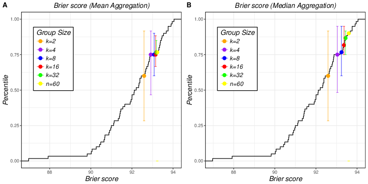
| Figure 1: Mean and median aggregation of transformed Brier scores of 5
different group sizes plotted on empirical cumulative distribution of
individual Brier scores (Figure 1A for mean aggregation and Figure 1B for
median aggregation). Error bars that match the colors of dots represent
90% empirical confidence interval of averaged aggregated Brier scores of
different group sizes. |
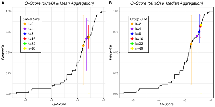
| Figure 2: Mean and median aggregation of Q scores of 50% CIs of 5
different group sizes plotted on empirical cumulative distribution of
individual Q scores of 50% CI (Figure 2A for mean aggregation and Figure
2B for median aggregation). Error bars that match the colors of dots
represent 90% empirical confidence interval of averaged aggregated Q
scores of 50% CI of different group sizes. |
The only exception is Q scores for 90% probability interval where the mean aggregation outperforms the median aggregation for k = 4, 8, 16 and 32.6 However, these differences are very small (smaller in absolute values than those for Q70% and Q50%) so, for all practical purposes the two aggregation methods perform identically in this case.
The second regularity is that, for all elicitation and aggregation methods, the larger group sizes have almost always higher scores than the smaller groups, suggesting that forecasting quality improves as a function of the number of forecasts being combined. The only exception is mean aggregation of hit rates of 50% probability intervals where dyads (k = 2) yields higher score than other groups sizes (k = 4, 8, 16 and 32).
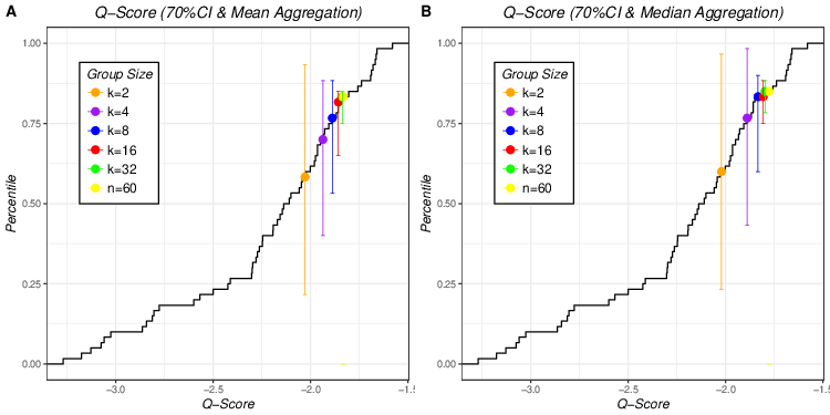
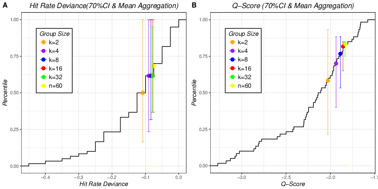
| Figure 3: Mean and median aggregation of Q scores of 70% CIs of 5 different
group sizes plotted on empirical cumulative distribution of individual Q
scores of 70% CI (Figure 3A for mean aggregation and Figure 3B for median
aggregation). Error bars that match the colors of dots represent 90%
empirical confidence interval of averaged aggregated Q scores of 70% CI of
different group sizes. |
| Figure 4: Mean and median aggregation of Q scores of 90% CI of 5 different
group sizes plotted on empirical cumulative distribution of individual Q
scores of 90% CIs (Figure 4A for mean aggregation and Figure 4B for median
aggregation). Error bars that match the colors of dots represent 90%
empirical confidence interval of averaged aggregated Q scores of 90% CI of
different group sizes. |
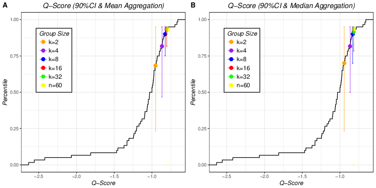
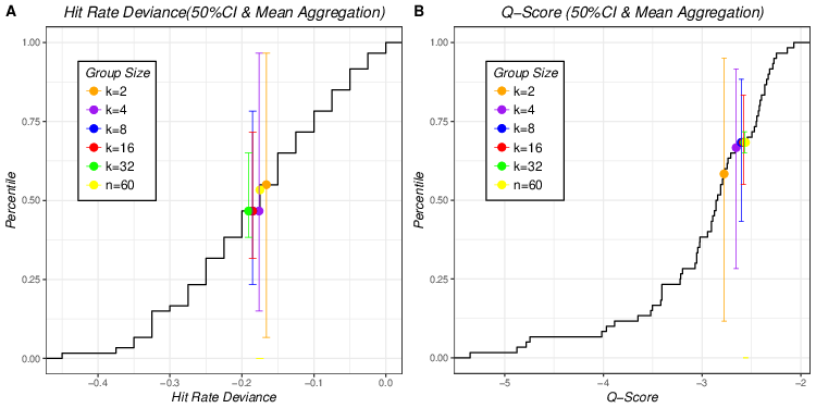
Figure 1 plots the aggregated Brier scores (means in Figure 1A and medians
in Figure 1B) of different group sizes (k = 2, 4, 8, 16 and 32) on
the empirical cumulative distribution of the individual Brier
scores. Different colored dots represent the aggregated Brier scores for
five different group sizes (orange for k = 2, purple for k = 4, blue for k = 8, red for k = 16 and green for k = 32). The error bars that match the colors of dots represent 90% empirical confidence intervals of averaged aggregated Brier scores of different group sizes. For example, in Figure 1A, the error bar of k = 4 (purple) ranges approximately from 0.50 to 0.91, which indicates that 90% of the aggregated Brier scores based on mean aggregation with group size of 4 fall in this range.
| Figure 5: Aggregated Brier scores, Q scores of 50% CI, 70% CI and 90% CI
of 5 different group sizes using mean (5A) and median aggregation (5B). |
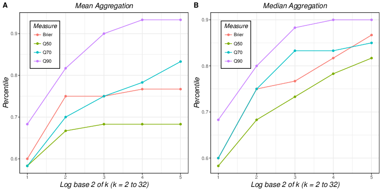
The key patterns observed in Table 2 – superior performance of median aggregation compared to mean aggregation, and monotonicity in group size – can also be clearly seen in the figure. Figure 1 also illustrates that the effect of group size is more salient in median aggregation where different colored dots are more spread out than in mean aggregation, where all the dots for k > 2 (red) are clumped together indicating similar forecast qualities. Comparison of error bars of the same color (equal group size) from Figure 1A and 1B does not show any particular pattern whereas comparison of different colored error bars show that the variation of the aggregated results is reduced when the group size increases for both mean and median aggregation.
Figure 2 shows aggregated Q scores for 50% probability intervals (means in Figure 2A and medians in Figure 2B) of different group sizes plotted on the empirical cumulative distribution of individual Q scores for 50% probability interval. The superiority of the median over the mean aggregation is demonstrated by two features. First, for the same group size, median aggregation leads to higher percentile than the mean aggregation. Second, the effect of group size is more pronounced for median aggregation. A visual inspection of the error bars confirms the conclusions from Figure 1, highlighting the group size effect on the width of 90% confidence intervals for both aggregation method.
Figures 3 and 4 plots the aggregated Q scores of 70% and 90% probability intervals in individual cumulative distribution (means in Figure 3A and Figure 4A and medians in Figure 3B and Figure 4B). The median aggregation yields equal, or higher, scores than the mean aggregation for aggregated Q scores of 70% (Figure 3), but this superiority does not hold for aggregated Q scores of 90% (Figure 4). In Figure 3, the different color dots are more spread out in mean aggregation (Figure 3A) than in median aggregation (Figure 3B) where aggregated performance of k = 8, 16 and 32 clump together. Therefore Figure 3 suggests a stronger group size effect for the mean, unlike the pattern seen for the Brier scores. In Figure 4 the positions of the same colored dots in left and right panels are quite similar, suggesting there is no significant difference in the group size effect between mean and median aggregation methods.
| Figure 6: Aggregated hit rates and Q scores of 50% CI of 5 different group
sizes plotted on empirical cumulative distribution of individual hit rates
and Q scores of 50% CIs using mean aggregation (Figure 6A for aggregated
hit rates of 50% CI and Figure 6B for aggregated Q scores of 50% CI). |
3.2 Which elicitation method benefits more from aggregation of forecasts: Point probabilities or probability intervals?
One could argue that the comparisons in first example could have been done without using the new metric. In this section we use the quantile method to compare forecasting performance of different measures based on different elicitation methods. More specifically, we compare point probabilities and probability intervals (three different widths 50%, 70% and 90% CIs). Such comparisons could not have been performed without invoking the quantile metric.
Figure 5A and 5B summarize aggregated forecasting quality of four measures (Brier
scores for point probability format and Q scores for 50%, 70% and 90%
for probability interval format) across different group sizes under mean
(Figure 5A) and median (Figure 5B) aggregation. The 90% probability
intervals yield the highest aggregated forecasting quality and 50%
intervals lead to the lowest aggregated performance with 70% probability
intervals and point probabilities lying in between. When the probabilities
were elicited by interval format, wider probability intervals benefit more
from aggregation compared to the narrower intervals, for both mean and
median aggregation: Percentile (Q90%) ≥ Percentile (Q70%)
≥ Percentile (Q50%). Part of the explanation for this pattern has
to do with the definition of the Q score itself that penalizes more heavily
narrow intervals. Assume the target variable has a standardized normal
distribution and our judge is perfectly calibrated (so only the first part
of the Q score matters), and predicts 50% intervals of width 1.35, 70%
intervals of width 2.07 and 90% intervals of widths 3.29. This judge would
be penalized −0.25*1.35 = −0.338 for the 50% interval, −0.15*2.07 =
−0.311 for the 70% intervals and 0.05*3.29 = −0.165 for the 90%
intervals.7 In addition, the inter-individual variance of the Q90% is higher than the variance of the narrower intervals, reflecting the higher variance for extreme cases, so the benefits of aggregation for Q50% and Q70% are more limited.
The ranking of the Brier scores and the Q scores for the 70% intervals varies slightly across aggregation methods and group sizes. More specifically, under mean aggregation point probabilities outperform 70% intervals based on smaller group sizes (k = 2, 4 and 8), yet it is defeated by 70% intervals for larger group sizes (k = 16 and 32). In contrast, when aggregated by the median, the point probabilities outperform 70% probability intervals when the group size equals 32. Moreover, when the group size is fixed, the variation of mean aggregation is larger than that of median aggregation, suggesting that the effect of elicitation format is more salient in mean aggregation than in median aggregation.
3.3 Do Q scores and hit rates based on the same intervals yield similar aggregated forecasting results? If not, which one benefits more from the aggregation?
The new quantile method can help “equate” various evaluation measures that are on different and unrelated scales by mapping them on the common percentile scale and facilitate comparisons among them. To illustrate this point we compared the aggregated performance of probability intervals calibrated by hit rate deviances and Q scores.
| Table 3: Mean Percentiles and Corresponding Empirical 90% CI of Aggregated Q Scores for 50% CI, 70% CI and 90% CI for Different Group Sizes Using Mean Aggregation. |
| | | 50% Probability Intervals | 70% Probability Intervals | 90% Probability Intervals |
| | | Mean | 90% CI | Width | | Mean | 90% CI | Width | | Mean | 90% CI | Width |
| k=2 | Q score | 0.583 | [0.117, 0.950] | 0.883 | | 0.583 | [0.233, 0.950] | 0.717 | | 0.683 | [0.233, 0.950] | 0.717 |
| | HR | 0.550 | [0.067, 0.967] | 0.900 | | 0.500 | [0.167, 1.000] | 0.833 | | 0.550 | [0.083, 1.000] | 0.917 |
| k=4 | Q score | 0.667 | [0.283, 0.950] | 0.667 | | 0.700 | [0.400, 0.900] | 0.500 | | 0.833 | [0.500, 0.950] | 0.450 |
| | HR | 0.467 | [0.150, 0.967] | 0.817 | | 0.617 | [0.233, 1.000] | 0.767 | | 0.600 | [0.233, 1.000] | 0.767 |
| k=8 | Q score | 0.683 | [0.400, 0.883] | 0.483 | | 0.750 | [0.533, 0.883] | 0.350 | | 0.933 | [0.750, 0.950] | 0.200 |
| | HR | 0.467 | [0.233, 0.783] | 0.550 | | 0.617 | [0.317, 1.000] | 0.683 | | 0.767 | [0.550, 1.000] | 0.450 |
| k=16 | Q score | 0.683 | [0.600, 0.833] | 0.233 | | 0.783 | [0.683, 0.850] | 0.167 | | 0.933 | [0.833, 0.950] | 0.117 |
| | HR | 0.467 | [0.317, 0.717] | 0.400 | | 0.700 | [0.367, 1.000] | 0.633 | | 0.767 | [0.600, 1.000] | 0.400 |
| k=32 | Q score | 0.683 | [0.650, 0.717] | 0.067 | | 0.833 | [0.750, 0.850] | 0.100 | | 0.933 | [0.917, 0.950] | 0.033 |
| | HR | 0.467 | [0.383, 0.650] | 0.267 | | 0.700 | [0.500, 0.950] | 0.450 | | 0.767 | [0.767, 1.000] | 0.233 |
| Figure 7: Aggregated hit rates and Q scores of 70% CI of 5 different group
sizes plotted on empirical cumulative distribution of individual hit rates
and Q scores of 70% CIs using mean aggregation (Figure 7A for aggregated
hit rates of 70% CI and Figure 7B for aggregated Q scores of 70% CI). |
| Figure 8: Aggregated hit rates and Q scores of 90% CI of 5 different group
sizes plotted on empirical cumulative distribution of individual hit rates
and Q scores of 90% CIs using mean aggregation (Figure 8A for aggregated
hit rates of 90% CI and Figure 8B for aggregated Q scores of 90% CI). |
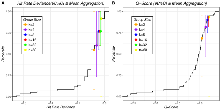
Figure 6 summarizes aggregated results for 50% probability intervals (hit rate deviances in Figure 6A and Q scores in Figure 6B) of different group sizes plotted on the corresponding individual cumulative distributions using mean aggregation. It is easy to observe that aggregated Q scores of 50% intervals benefit from aggregation more (have higher percentile scores) than the corresponding aggregated hit rate deviances across all group sizes (dots of the right panel always yield higher y-axis values than the same colored dots of the left panel). The error bars of aggregated hit rate deviances are wider than those of the corresponding aggregated Q scores for all group sizes (see Table 3). This suggests that for 50% probability intervals, aggregated hit rate deviances might produce less “stable” forecasting performance than Q score. Lastly, one unusual pattern of group size effect is observed in Figure 6A: group size of 2 yields highest percentile and exceeds all other group sizes (k = 4, 8, 16 and 32) even the aggregated forecast including all subjects (n = 60).
Figures 7 and 8 display results for 70% and 90% probability intervals, respectively. Similar to Figure 6, aggregated Q scores yield higher percentiles than aggregated hit rate deviances for all group sizes for both probability intervals and Q scores are more stable, as their narrower error bars indicate.
The general superiority of the aggregated scores Q-scores can be attributed to the fact that they include more information (coverage and magnitude of over- and under-estimates) and the inter-judge variance of the Q-scores is considerably higher than their hit rate counterparts. The benefits of aggregating Q-scores reflects the ability to reduce this variance effectively. Interestingly, both measures perform better (higher percentile scores) as the confidence level increases, replicating findings from the previous example.
3.4 Under what circumstances, should one look for experts rather than aggregate multiple individual forecasts?
The quantile metric can also address another question that comes up often in forecasting contexts: Should one select a random sample of k judges and aggregate their forecasts, or should one seek a few, properly selected, “experts” and rely on their judgments (e.g., Larrick & Soll, 2006). Conceptually, one can frame this as a choice between “quantity” and “quality”. Naturally, the answer depends on several parameters such as the value of k, the nature of the aggregation function and, importantly, on one’s ability to reliably identify expertise. The quantile metric is exceptionally well suited to address this question.
Consider a case where one seeks to forecast 70% probability intervals of a
target variable and uses the Q score as the measure of quality of
forecasts. The results in Table 3 indicate that taking the mean of
k = 16 forecasters would, on average, beat 78.3% of the
individual forecasters and there is a 95% chance of outperforming 68.3%
of them (based on the lower bound of the 90% CI). Thus, it makes sense to
seek an expert if, and only if, one can reliably identity the top (100 − 68.3 =) 31.7% forecasters and choosing one of them. Otherwise, it is better to rely on the average of k = 16 randomly selected judges. The ability to identify top forecasters based on their past performance depends on the stability of the performance over time. Assuming that the performance of the judges at times t1 and t2 follows a bi-variate normal distribution with a correlation of ρ, it is possible to calculate the chance that a judge who is in the top X% at t1 would also be in the same category at t2. Table 4 summarizes these probabilities for X = 20% and 30% and for ρ’s ranging from 0.5 to 0.9. Overall, the chances of finding an expert who will beat the mean of k = 16 forecasters at t2, based on the fact that she did this at t1, are quite low and they do not favor chasing the experts.
To further investigate this issue, we ran a small simulation using the Budescu and Du (2007) data. We randomly split the 40 stocks into two subsets of 20 each, and identified the top forecasters, as measured by their Brier scores, in each subset. We first identified top performers from the training set (subset 1 or 2) and compared their performance in the testing set (subset 2 or 1, respectively) with the performance of the two aggregation rules (mean and median) of the same set. We replicated the process with 100 different random assignments of stocks into two subsets and averaged their quantile metric scores over 200 trials (100 random assignments × 2 subsets). The median (Kendall) rank correlation between the two rankings of the 60 judges across the 100 replications is 0.30, and 90% of these correlations are between 0.11 and 0.48.
| Table 4: Probability That a Judge Who Is in the Top X% at t1 Would Also Be in the Top X% at t2 for Different Bivariate Normal Distributions. |
| ρ(t1, t2) | Top 30% | Top 20% |
| 0.5 | 0.157 | 0.087 |
| 0.6 | 0.173 | 0.099 |
| 0.7 | 0.190 | 0.113 |
| 0.8 | 0.211 | 0.129 |
| 0.9 | 0.237 | 0.15 |
| Table 5: Performance of Top Judges and Mean & Median Aggregations |
| Rule | Mean Quantile Score | 95% CI |
| Top 5% Judges | 0.641 | [.619 - .663] |
| Top 10% Judges | 0.711 | [.696 - .726] |
| Top 15% Judges | 0.750 | [.737 - .763] |
| Top 20% Judges | 0.765 | [.753 - .777] |
| Mean of k = 60 | 0.747 | [.741 - .753] |
| Median of k = 60 | 0.830 | [.823 - .837] |
For each trial, the performances of top judges (top 5%, 10%, 15% and 20%) in the testing set were mapped onto the cumulative distribution of individual Brier scores of the same set and corresponding quantile scores were obtained. The mean and 95% empirical CI of these quantile scores were computed based on the results of 200 trials separately for top 5%, 10%, 15% and 20% and presented in Table 5.
Table 5 shows that the median aggregation handily beats all competitors and the mean also beats most attempts to select experts. The only exception is that the top 20% of the judges are slightly better than the mean.
3.5 Does extremization improve the accuracy of aggregated forecasts?
In the previous analyses, we combined raw probability estimates, but this is not always the most effective approach. Aggregation can benefit from transforming the original judgements, using some predefined function, and aggregating the transformed estimates. Various transformation methods have been proved to enhance the aggregated forecasting accuracy (Ariely et al. 2000; Baron et al., 2014; Satopää et al., 2014; Mandel, Karvetski & Dhami, 2018; Turner, Steyvers, Merkle, Budescu & Wallsten, 2014). The quantile metric can also be used to evaluate the effectiveness of these transformations. We will use one common transformation method, extremization, as an example. Extermization pushes probabilities to be closer to 0 or 1 (become more extreme) by applying functions such as:
Baron et. al (2014) justifies such transformation to counter two
distorting factors – end-of-scale effects8 and forecasters’ tendency to confuse and conflate individual confidence with confidence in the best forecast – and showed that the extremization function in (5) can reduce both, and contribute to more accurate aggregated forecasts (see also Turner, 2014).
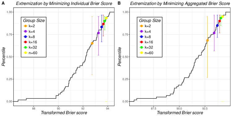
| Figure 9: Aggregated point probabilities under two extremization approaches
(Figure 9A for extremization based on α1 and Figure 9B for extremization
based on α2). |
| Table 6: Performance of Two Extremization Methods and Median Aggregation of Raw Forecasts. |
| Transformation | Brier | Percentile | | |
| 3*2 | No Transformation | 0.148 | 0.600 | 0.283 | 0.917 |
| | Minimizing individual Brier | 0.145 | 0.667 | 0.283 | 0.983 |
| | Minimizing aggregated Brier | 0.145 | 0.667 | 0.217 | 1 |
| 3*4 | No Transformation | 0.139 | 0.750 | 0.500 | 0.950 |
| | Minimizing individual Brier | 0.135 | 0.767 | 0.517 | 1 |
| | Minimizing aggregated Brier | 0.132 | 0.833 | 0.517 | 1 |
| 3*8 | No Transformation | 0.135 | 0.767 | 0.600 | 0.950 |
| | Minimizing individual Brier | 0.130 | 0.883 | 0.700 | 1 |
| | Minimizing aggregated Brier | 0.126 | 0.917 | 0.717 | 1 |
| 3*16 | No Transformation | 0.132 | 0.850 | 0.700 | 0.950 |
| | Minimizing individual Brier | 0.127 | 0.900 | 0.750 | 1 |
| | Minimizing aggregated Brier | 0.122 | 0.967 | 0.8 | 1 |
| 3*32 | No Transformation | 0.131 | 0.883 | 0.767 | 0.917 |
| | Minimizing individual Brier | 0.125 | 0.917 | 0.867 | 0.983 |
| | Minimizing aggregated Brier | 0.199 | 0.983 | 0.900 | 1 |
| 3*60 | No Transformation | 0.128 | 0.900 | — | — |
| | Minimizing individual Brier | 0.122 | 0.950 | — | — |
| | Minimizing aggregated Brier | 0.116 | 1 | — | — |
We applied the same transformation function (Equation 5) to the point probability estimates in the Budescu and Du (2007) data and used two different approaches to estimate the parameter α in Equation 5. First, we estimated α for each forecaster by finding the value that minimizes individual Brier score (computed from probability estimates of 40 stocks), and we used the median of these 60 individual αs to transform all the original probability judgements using this α1 = 1.211.9 For the second method, we estimated the parameter α by minimizing aggregated Brier score with median aggregation. Then, all raw probability estimates were extremized more severely with optimal α2= 2.169.
We applied the Quantile method, as in the previous analyses, using the median aggregation, which we showed to be superior. We emphasize that the aggregated Brier score of the transformed probabilities was mapped onto the cumulative distribution of Brier scores of raw probability estimates (not onto the distribution of individual Brier scores of transformed probabilities). Thus the aggregated extremized forecasts can be directly compared to the original ones.
Figure 9 compares the two extremization approaches. It shows that the second approach (based on α2 that was estimated by minimizing aggregated Brier score) was slightly, but systematically, better than the approach using α1 for all group sizes. Comparison with Figure 1B (median aggregation of point forecasts without extremization) shows that both transformations improved aggregated forecasting quality compared to the median aggregation of the original probabilities, for all group sizes. A complete and detailed comparison among three conditions (two extremizations and original median aggregation) is presented in Table 6.
4 Discussion
We proposed a new, easy-to-implement, use and interpret comparison based on the quantile metric and illustrated its application to answer various research questions using the data from the experiment of Budescu and Du (2007). The quantile metric was applied to compare (a) different aggregation methods (mean and median) and aggregation group sizes (k = 2, 4, 8, 16 and 32), (b) different forecasts and elicitation methods (point probability estimates and probability intervals), (c) different calibration measures based on the same judgments (Q scores and hit rates), (d) performance of top experts and aggregation of individuals, (e) aggregates based on raw and extremized judgments. These examples not only showed the versatility of quantile metric that can be easily and efficiently applied to various circumstances, but also led to some meaningful findings about aggregated forecasting qualities.
First, we illustrated the superiority of median aggregation over mean aggregation for both point probabilities and 50% and 70% probability intervals when all other conditions were fixed. This finding is consistent with Park and Budescu’s (2015) re-analysis of the Budescu and Du (2007) data (only 90% probability intervals). Park and Budescu (2015) used a slightly different approach by comparing hit rates obtained from different aggregation methods and found that median aggregation produced hit rates that were closer to the target confidence level than the means for all group sizes. Similarly, Hora et al. (2013) also demonstrated that the median aggregate is better calibrated than the mean when the judges are independent and well-calibrated.
A second regularity uncovered was that larger groups yield, systematically, better aggregated performance for all aggregation, elicitation and calibration methods.10 Typically the gains in performance diminish as the group size increases and, typically, there are only little gains to aggregating more than 16 forecasters. However, we also found out an interactive pattern — the impact of group size varies across aggregation methods, suggesting that one can optimize the process, i.e., maximize accuracy at minimal cost, by, simply, selecting the most appropriate aggregation method for a given problem.
A comparison of forecasting quality of aggregated probability-intervals with different confidence targets suggests that performance is sensitive to the desired level of confidence. We found that in all cases and everything else being equal one can achieve higher benefits of aggregation for wider intervals (90%) than for narrower ones (e.g. 50%).
The comparison of different evaluation measures of the same forecasts by the same elicitation method and the same group of judges, documented systematic differences between the different evaluation measures that are based on different scales. Aggregation of Q scores produced "higher", and more "stable" forecasting results, than aggregating hit rate deviances for all group sizes for 50%, 70% and 90% probability intervals. This result reaffirms that hit rate and Q score measure slightly different aspects, but it also indicates that the benefits of aggregation across multiple judges are magnified for Q scores.
Lastly, a comparison of aggregation based on raw and extremized forecasts
using the same one-parameter function proposed by Baron et al. (2014) and confirmed the benefits of extremization (also presented by Turner et al., 2014).
The newly proposed quantile metric is flexible enough to allow comparisons between different combinations of elicitation, calibration and aggregation methods. For example, by referring to Table 2, one can find matching percentile scores obtained from different sets of conditions (e.g., percentile score of mean aggregation of Q90% in groups of size 4, is equivalent to the percentile score of median Brier scores in groups of size 16). Such comparison can help identify the most appropriate set of forecasting conditions. For example, for Brier scores, aggregated forecasting performance of a group size of 8 using median method is similar to that of a group size 32 using mean method (both yielded quantile score of 0.767). Therefore choosing median aggregation over mean method can reduce effort and cost of forecasting by a factor of (32/8=) 4. Similarly, when all the other conditions are fixed, the quantile method can help finding the optimal group size. For example, the mean hit rate of 90% intervals does not improve as group size increases beyond k = 8, so we can conclude that k = 8 is the optimal group size in this context.
Interpretation of quantile score is more meaningful compared to direct interpretation of calibration measures, especially for evaluation measures do not have meaningful units, such as Brier score and others that have scale-dependent measures, such as the Q scores. When we compare directly aggregated performance using raw scores of calibration measures (e.g., Q score), we can easily determine the magnitude, however, no further interpretation of the numerical difference is available because these measures do not necessarily have meaningful units. For example, Table 2 shows that when k = 32, the median aggregation obtained a Q50% score of −2.400 which is clearly closer to 0 than a Q50% score of −2.568 obtained from the mean aggregation, suggesting that the median yields better forecasts that the mean. Yet it is hard to determine the meaning of this difference of 0.168 in the Q-scale. However if we convert them into quantiles (Q50% score of −2.400 is converted to quantile score of 0.817 and Q50% score of −2.568 is converted to quantile score of 0.683), it is easy and meaningful to interpret the difference between the two aggregation methods: the median forecasts is as good, or better, than 81.7% individual forecasters and the mean aggregate outperforms 68.3% of the individual forecasters. Thus using the median beats 13.4% more individual forecasters than the mean.
Next, we list some recommendations for the future use of the new metric.
The quantile metric is not an absolute measure, but relies on the
individual cumulative distribution, so in order to make valid comparisons,
it is important to map aggregated performance obtained from different
forecasting conditions on the same, or equivalent, cumulative
distributions. Thus, the quantile scores used to compare aggregated
performance of different forecasting conditions should be obtained from (1)
cumulative distributions from the within-subject design, using the same individuals (each forecaster reports multiple forecasts under different forecasting conditions) or (2) cumulative distributions from equivalent groups of individuals which are based on either random assignment or matched assignment of judges to different forecasting conditions.
Second, this method should not be used when the sample size is too small. The quantile metric is based on individual cumulative distributions and a small number of data points will lead to relatively crude, and possibly, misleading, results.
Third, a high percentile score does not necessarily imply high forecasting
performance thus interpretation of quantile score should be careful. The
quantile score is a relative measure, indicating the position of a
forecasting result in the individual cumulative distribution. Consider a
situation where all forecasters provided extremely poor forecasts, say they
are all biased in one direction (either all severely overconfident or
underconfident). Some aggregates will yield a high percentile score,
indicating that they are better than most individuals. However, this
percentile score should not be interpreted as high forecasting performance
because the aggregated estimate itself is also biased. We recommend that
the quantile score should be interpreted in conjunction with raw calibration measures that can provide information about absolute magnitude of forecasting quality.
Lastly, we list some directions for future research and extensions. The first, and most natural, direction is to apply the new methodology to more aggregation methods and various calibration measures in distinct domains to obtain more comprehensive conclusions about the relative merit of various aggregation methods and calibration measures on the overall quality of the aggregates. One interesting case is the surveys of expert forecasters collected by the European Central Bank (ECB; Garcia, 2003) and the Federal Reserve Bank of Philadelphia (Croushore, 1993). They involve (1) multiple macroeconomic indicators, such as inflation, unemployment and GDP growth rate and (2) pertain to multiple time horizons, e.g., next quarter, next year, etc.), so it may be useful to use our metric to identify the single best approach across all indicators and time horizons.
The method can be extended by using cumulative distribution functions of certain parametric forms, such as the normal distribution, as an alternative mode to obtain percentile scores, possibly in cases where the available samples are small. Another interesting direction is to re-analyze previous comparison studies that used method-specific metrics to verify that their conclusions about the quality of different aggregation methods and forecasting conditions are replicated using this new universal method.
References
Abbas, A. E., Budescu, D. V., Yu, H. T., & Haggerty, R. (2008). A comparison of two probability encoding methods: Fixed probability vs. fixed variable values. Decision Analysis, 5(4), 190–202. http://dx.doi.org/10.1287/deca.1080.0126.
Alpert, M., & Raiffa, H. (1982). A progress report on the training of probability assessors. In D. Kahneman, P.Slovic & A. Tversky (Eds.), Judgment under Uncertainty: Heuristics and Biases (pp. 294–305). Cambridge, England: Cambridge University Press. http://dx.doi.org/10.1017/CBO9780511809477.022.
Ariely, D., Tung Au, W., Bender, R. H., Budescu, D. V., Dietz, C. B., Gu, H., Wallsten T. S., & Zauberman, G. (2000). The effects of averaging subjective probability estimates between and within judges. Journal of Experimental Psychology: Applied, 6(2), 130–147. http://dx.doi.org/10.1037/1076-898X.6.2.130.
Armstrong, J. S., & Collopy, F. (1992). Error measures for generalizing about forecasting methods: Empirical comparisons. International Journal of Forecasting, 8(1), 69–80. http://dx.doi.org/10.1016/0169-2070(92)90008-W.
Baron, J., Mellers, B. A., Tetlock, P. E., Stone, E., & Ungar, L. H. (2014). Two reasons to make aggregated probability forecasts more extreme. Decision Analysis, 11(2), 133–145. http://dx.doi.org/10.1287/deca.2014.0293.
Budescu, D. V., & Chen, E. (2015). Identifying expertise and using it to extract the Wisdom of the Crowds. Management Science, 61(2), 267–280. http://dx.doi.org/10.1287/mnsc.2014.1919.
Budescu, D. V., & Du, N. (2007). Coherence and consistency of investors’ probability judgments. Management Science, 53(11), 1731–1744. http://dx.doi.org/10.1287/mnsc.1070.0727.
Budescu, D.V, & Park, S. (2016). Subjective prediction intervals for events involving internal and external sources of uncertainty. Manuscript submitted for publication.
Chen, E., Budescu, D. V., Lakshmikanth, S. K., Mellers, B. A., & Tetlock, P. E. (2016). Validating the contribution-weighted model: Robustness and cost-benefit analyses.
Decision Analysis, 13(2), 128–152. http://dx.doi.org/10.1287/deca.2016.0329.
Croushore, D. (1993). Introducing: The Survey of Professional Forecasters. Business Review - Federal Reserve Bank of Philadelphia 3, November/ December, 3–15.
Davis-Stober, C.P., Budescu, D.V., Dana, J., & Broomell, S.B. (2014). When is a crowd wise? Decision, 1(2), 79–101.
Erev, I., Wallsten, T. S., & Budescu, D. V. (1994). Simultaneous over- and underconfidence: The role of error in judgment processes.
Psychological Review, 101(3), 519–527. http://dx.doi.org/10.1037/0033-295X.101.3.519.
Fischhoff, B., Slovic, P., & Lichtenstein, S. (1977). Knowing with certainty: The appropriateness of extreme confidence. Journal of Experimental Psychology: Human Perception and Performance, 3(4), 552–564. http://dx.doi.org/10.1037/0096-1523.3.4.552.
Gaba, A., Tsetlin, I., & Winkler, R. L. (2017). Combining interval forecasts.
Decision Analysis, 14(1), 1–20. http://dx.doi.org/10.1287/deca.2016.0340.
Garcia, J. A. (2003). An introduction to the ECB’s Survey of Professional Forecasters.
Occasional Paper Series, No 8. Frankfurt am Main, Germany: European Central Bank.
Gilovich, T., Griffin, D. W., & Kahneman, D. (2002).
Heuristics and Biases: The Psychology of Intuitive Judgment. Cambridge University Press, Cambridge, UK. https://doi.org/10.1017/CBO9780511808098.
Grushka-Cockayne, Y., Jose, V. R. R., Lichtendahl Jr. K. C., & Winkler, R. L. (2017). Quantile evaluation, sensitivity to bracketing, and sharing business payoffs. Operations Research, 65(3), 712–728.
Haran, U., Moore, D. A., & Morewedge, C. K. (2010). A simple remedy for overprecision in judgment.
Judgment and Decision Making, 5(7), 467–476.
Hora, S. C., Fransen, B. R., Hawkins, N., & Susel, I. (2013). Median aggregation of distribution functions. Decision Analysis, 10(4), 279–291.
Hyndman, R. J., & Koehler, A. B. (2006). Another look at measures of forecast accuracy.
International Journal of Forecasting, 22(4), 679–688.
Jose, V. R. R., & Winkler, R. L. (2009). Evaluating quantile assessments.
Operations Research, 57(5), 1287–1297. http://dx.doi.org/10.1287/opre.1080.0665.
Juslin, P., Wennerholm, P., & Olsson, H. (1999). Format dependence in subjective probability calibration.
Journal of Experimental Psychology: Learning Memory and Cognition, 25(4), 1038–1052. http://dx.doi.org/10.1037/0278-7393.25.4.1038.
Klayman, J., Soll, J., González-Vallejo, C., & Barlas, S. (1999). Overconfidence: It depends on how, what, and whom you ask.
Organizational Behavior and Human Decision Processes, 79(3), 216–247. http://dx.doi.org/10.1006/obhd.1999.2847.
Langnickel, F., & Zeisberger, S. (2016). Do we measure overconfidence? A closer look at the interval production task.
Journal of Economic Behavior and Organization, 128, 121–133. http://dx.doi.org/10.1016/j.jebo.2016.04.019.
Larrick, R. P., & Soll, J. B. (2006). Intuitions about combining opinions: misappreciation of the averaging principle. Management Science, 52(1), 111–127. http://dx.doi.org/10.1287/mnsc.1050.0459.
Larrick, R. P., Mannes, A. E., & Soll, J. B. (2011). The social psychology of the wisdon of crowds. In J. I. Krueger (Ed.), Social Judgement and Decision Making, (pp. 227–242). New York, NY: Psychology Press.
Mandel, D. R., Karvetski, C. W., & Dhami, M. K. (2018). Boosting intelligence analysts’ judgment accuracy: What works, what fails?
Judgment and Decision Making, 13(6), 607–621.
McKenzie, C. R. M., Liersch, M. J., & Yaniv, I. (2008). Overconfidence in interval estimates: What does expertise buy you?
Organizational Behavior and Human Decision Processes, 107, 179–191. http://dx.doi.org/10.1016/j.obhdp.2008.02.007.
Merkle, E. C., & Steyvers, M. (2013). Choosing a strictly proper scoring rule.
Decision Analysis, 10(4), 292–304. http://dx.doi.org/10.1287/deca.2013.0280.
Murphy, A. H. (1973). A new vector partition of the probability score.
Journal of Applied Meteorology, 12(4), 595–600.
Park, S., & Budescu, D. V. (2015). Aggregating multiple probability intervals to improve calibration.
Judgment and Decision Making, 10(2), 130–143.
Fletcher, R., & Reeves, C. M. (1964). Function minimization by conjugate gradients.
The Computer Journal, 7(2), 149–154. https://doi.org/10.1093/comjnl/7.2.149.
Satopää, V. A., Baron, J., Foster, D. P., Mellers, B. A., Tetlock, P. E., & Ungar, L. H. (2014). Combining multiple probability predictions using a simple logit model.
International Journal of Forecasting, 30(2), 344–356. http://dx.doi.org/10.1016/j.ijforecast.2013.09.009.
Soll, J. B., & Klayman, J. (2004). Overconfidence in interval estimates.
Journal of Experimental Psychology: Learning, Memory, and Cognition, 30(2), 299–314. http://dx.doi.org/10.1037/0278-7393.30.2.299.
Soll, J. B., & Larrick, R. P. (2009). Strategies for revising judgment: How (and how well) people use others’ opinions.
Journal of Experimental Psychology: Learning, Memory, And Cognition, 35(3), 780–805. http://dx.doi.org/10.1037/a0015145.
Teigen, K. H., & Jøgensen, M. (2005). When 90% confidence intervals are 50% certain: on the credibility of credible intervals.
Applied Cognitive Psychology, 19(4), 455–475. http://dx.doi.org/10.1002/acp.1085.
Turner, B. M., Steyvers, M., Merkle, E. C., Budescu, D.V., & Wallsten, T. S. (2014). Forecast aggregation via recalibration.
Machine Learning, 95, 261–289. http://dx.doi.org/10.1007/s10994-013-5401-4.
Wallsten, T. S., Shlomi, Y., Nataf, C., & Tomlinson, T. (2016). Efficiently encoding and modeling subjective probability distributions for quantitative variables.
Decision, 3(3), 169–189. http://dx.doi.org/10.1037/dec0000047.
Whitfield, R., & Wallsten, T. (1989). A risk assessment for selected lead‐induced health effects: An example of a general methodology.
Risk Analysis, 9(2), 197–207. http://dx.doi.org/10.1111/j.1539-6924.1989.tb01240.
Yates, J. F. (1990). Judgment and Decision Making. Englewood Cliffs, NJ: Prentice Hall
This document was translated from LATEX by
HEVEA.