Judgment and Decision Making, Vol. 13, No. 4, July 2018, pp. 322-333
Testing the ability of the surprisingly popular method to predict NFL gamesMichael D. Lee*
Irina Danileiko#
Julie Vi# |
We consider the recently-developed “surprisingly popular” method
for aggregating decisions across a group of people (Prelec, Seung
and McCoy, 2017). The method has shown impressive performance in a
range of decision-making situations, but typically for situations in
which the correct answer is already established. We consider the
ability of the surprisingly popular method to make predictions in a
situation where the correct answer does not exist at the time people
are asked to make decisions. Specifically, we tested its ability to
predict the winners of the 256 US National Football League (NFL)
games in the 2017–2018 season. Each of these predictions used
participants who self-rated as “extremely knowledgeable” about the
NFL, drawn from a set of 100 participants recruited through Amazon
Mechanical Turk (AMT). We compare the accuracy and calibration of
the surprisingly popular method to a variety of alternatives: the
mode and confidence-weighted predictions of the expert AMT
participants, the individual and aggregated predictions of media
experts, and a statistical Elo method based on the performance
histories of the NFL teams. Our results are exploratory, and need
replication, but we find that the surprisingly popular method
outperforms all of these alternatives, and has reasonable
calibration properties relating the confidence of its predictions to
the accuracy of those predictions.
Keywords: surprisingly popular method, wisdom of the crowd, sporting predictions, expertise, majority rule
Note: A correction has been made to this article as of Nov. 25, 2018.
1 Introduction
(Prelec et al., 2017) recently proposed the “surprisingly popular”
method for aggregating multiple-choice decisions over a group of
people. The method is motivated by the challenge of finding an
accurate answer to a single question, especially in situations where
many people in the group could believe in the wrong answer. For
example, if asked whether Seattle is the capital city of the state of
Washington, many people mistakenly answer “yes”. The key feature of
the surprisingly popular method is that, as well as providing their
answer, people are asked to estimate what percentage of other people
they expect will also give the same answer. Thus, if somebody knows
the capital of Washington is Olympia, but also realizes that most
people mistakenly believe it is Seattle, both of these pieces of
information can be expressed.
The surprisingly popular method combines the cognitive judgment (the
basic decision) and the meta-cognitive judgment (the estimate of the
decisions of others) by comparing the expected and observed
proportions of people making a decision. The observed proportion is
simply how many say “yes” to Seattle being the capital. The expected
proportion combines the estimated percentages for those who say both
“yes” and “no”. A person who says “yes” and expects 90% of
people to agree contributes to the expected proportion in the same way
as person who says “no” but expects only 10% to agree. The final
decision made by the surprisingly popular method compares the observed
and expected proportions, and chooses the answer that has more
observed agreement than is expected (i.e., the answer that is
“surprisingly popular”). Intuitively, people who believe Seattle is
the capital of Washington will tend to believe others will say the
same, while those who know it is not will expect others to
disagree. Thus, the expected agreement is very high, but the observed
agreement is lower, because some knowledgeable people say “no”. This
means “no” will be the surprisingly popular answer.
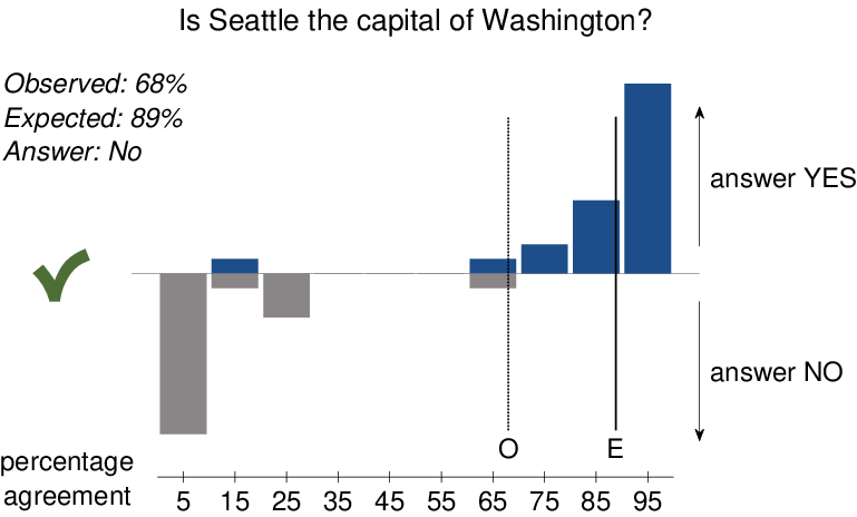
| Figure 1: An example of the surprisingly popular method choosing the
correct minority answer for the question “Is Seattle the capital of
Washington?” The upper (blue) distribution shows the meta-cognitive
estimates of agreement, in 10% bins centered from 5% to 95%,
provided by people who answered “yes”. The lower (gray)
distribution shows, on a downward oriented y-axis, the
meta-cognitive estimates of agreement provided by people who
answered “no”. The proportion of observed “yes” answers and the
proportion of expected “yes” answers based on these data are shown
by vertical lines, and listed. Also listed is the answer of the
surprisingly popular method, which is “no” because the observed
proportion is less than expected. The tick mark indicates the answer
is correct. |
Figure 1 provides a concrete
demonstration of the operation of the surprisingly popular method,
based on data for the Seattle question reported by
(Prelec et al., 2017). It uses a visual display that shows the
decisions and meta-cognitive estimates of agreement that people made,
and the expected and observed levels of agreement that produce the
final decision. The two bar graphs show the distribution of
meta-cognitive judgments. The distribution of estimated agreement from
participants answering that Seattle is the capital of Washington is
shown by the upper (blue) distribution, while the distribution of
estimated agreement from participants answering that Seattle is not
the capital of Washington is shown by the lower (gray)
distribution. Each bar in these distributions correspond to a 10%
range in the meta-cognitive estimates. The total of the upper bars
corresponds to how many people answered “yes”, while the total of
lower bars corresponds to how many people answered “no”.
The solid and broken vertical lines in
Figure 1 show, respectively, the expected
“E” and observed “O” levels of agreement calculated from the
decisions and meta-cognitive estimates. A majority of 68% of people
answered that Seattle was the capital, but the expected agreement was
89%, leading the surprisingly popular method to give the correct
answer that Seattle is not the capital of Washington. The key
contribution to the relatively high expected value is evident from the
distributions of meta-cognitive judgments. The large lower gray bar at
5% indicates that a significant number of people who answered “no”
expected that fewer than 10% of others would agree with
them. Intuitively, these people know that Seattle is not the capital,
but also know they are in a minority. Their meta-cognitive estimates
allow the surprisingly popular method to side with the minority.
(Prelec et al., 2017) evaluate the accuracy of the surprisingly
popular method in a number of domains, including trivia and general
knowledge questions, medical diagnoses, and art price category
evaluations. For all of these domains, the surprisingly popular method
achieves impressive levels of accuracy, outperforming standard
alternatives like the majority answer, and the answer in which people
express the greatest overall confidence. While the trivia and general
knowledge domains have limited real-world applicability — outside
the confines of a trivia competition, it is possible simply to look up
the answers — the medical diagnosis and art evaluation domains
clearly could have real-world application. In both cases, an accurate
decision based on cheap and simple behavioral judgments is a useful
capability, since determining the true answer involves expensive
medical testing in the first case, and time-consuming and complicated
mechanisms like auctions in the second case.
Perhaps the most interesting and important potential application of
the surprisingly popular method, however, is to situations requiring
genuine prediction, such as geopolitical forecasting or sporting
predictions (Silver, 2012,TetlockGardner, 2016), where the true
answer is in principle not knowable at the time people make
decisions. None of the domains considered by (Prelec et al., 2017) are
of this type, unless the argument is made that the value of art does
not exist until it is socially constructed by an auction or some other
valuation mechanism. Given this gap in evaluation, our goal is to
provide a direct predictive test of the surprisingly popular method,
by evaluating its performance forecasting the outcome of the 256 games
played in the regular season of the US National Football League (NFL)
in the 2017-2018 season.
The structure of this paper is as follows. We first describe the
empirical data, collecting people’s predictions, on which our
evaluation of the surprisingly popular method is based, and the
benchmark prediction data we use to assess performance. We then
analyze the empirical and benchmark data from a number of
perspectives, including overall accuracy, the relationship of the
surprisingly popular method’s predictions to those made by other
methods, and the calibration between confidence and accuracy. We
discuss insights into the potential applicability of the surprisingly
popular method suggested by our findings, and a number of avenues for
extending its empirical evaluation as well as improving its ability to
make predictions.
2 Data
The NFL regular season involves 256 games, with each of 32 teams
playing 16 games over a 17-week season, and each team having one bye
week. This means that there are between 13 and 16 games each week,
depending on how many teams have byes that week.
2.1 Experimental Data
During the 2017–2018 season we collected predictions each week on
Wednesday. These predictions were made about every game for that week,
which were typically played from Thursday night to the following
Monday night. Each week the predictions were made by 100 participants
recruited using the Amazon Mechanical Turk (AMT) system, with data
collected using the Qualtrics survey system. Different participants
were recruited for each week and all were paid US $1.
Participants first provided basic demographic information including
their gender, and their age range from the options 18–24, 25–34,
35–44, 45–54, 55–64, and 65+ years. They then rated their knowledge
of NFL football on a 5-point scale: extremely knowledgeable, very
knowledgeable, moderately knowledgeable, slightly knowledgeable, and
not knowledgeable at all. To make predictions about each game,
participants first made a prediction about which team they believed
would win, then they rated their confidence in this prediction on a
5-point scale: guess, low confidence, moderate confidence, high
confidence, and very high confidence. Finally, participants estimated
the percentage of others they believed would agree with their
prediction. This percentage estimation was done with a slider that
showed the exact integer from 0 to 100 being selected as the slider
was moved, as well as permanent indicators 0, 10, …, 100 on a
scale.
Once a participant had completed these three behavioral responses —
their prediction, confidence rating, and meta-cognitive estimation of
agreement — for a game, they pressed an “advance” button to move
to the next game. They could adjust the three behavioral responses for
a specific game while it was the current game, but could not return to
an earlier game once they had advanced. Each participant made
predictions about the games in a randomly-determined order. A
screenshot of the experimental interface is available in the on-line
supplementary material.
2.2 Benchmark Data
We also collected benchmark predictions for the 256 games coming from
two other sources. One benchmark source was the collation of media
expert predictions provided by nflpickwatch.com. These
predictions take the form of binary selections for each game. We use
the data from 94 experts who provided predictions for all, or almost
all, of the 256 games over the season.
The other benchmark data source is provided by the data-science
forecasting website fivethirtyeight.com. These predictions are
made by an algorithm that is a variant1 of the Elo statistical method used to
measure performance in chess (Elo, 1978). This benchmark is not
based on human judgments, but on the history of game results for the
NFL teams. The Elo predictions are probabilistic and take the form of
winning percentages for each team.
3 Results
We first analyze the overall accuracy of our AMT participants relative
to the media expert benchmark predictions. We find that the sub-group
of our participants who self-rated their NFL knowledge as “extremely
knowledgeable” have a similar distribution of accuracy to the media
experts. Accordingly, we apply the surprisingly popular method, and
the other prediction methods based on human judgments, to this
sub-group of expert AMT participants. We then compare the
effectiveness of these predictions to the media experts and Elo
benchmarks, considering first overall accuracy, then patterns of
agreement and disagreement between predictions, and finally the
calibration of the predictions.
3.1 Accuracy by Expertise
Figure 2 examines the behavior of the AMT
participants, in terms of the accuracy of their predictions, the
relationship between their confidence ratings and accuracy, and the
calibration of their meta-cognitive estimates of agreement.
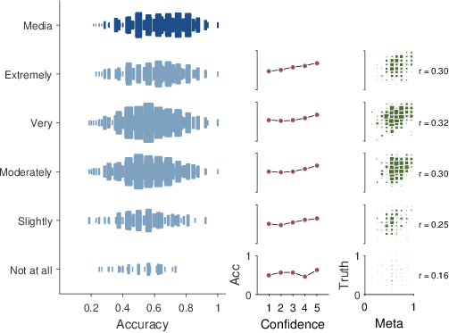
| Figure 2: The left panel shows the distribution of prediction accuracy
for six different groups of people. At the top is the distribution
for media experts and below are the distributions for AMT
participants with different levels of self-rated overall
knowledge. The middle panels shows the relationship between accuracy
and confidence ratings for each self-rated knowledge group. The
right panels show the relationship between the meta-cognitive
estimate and true level of agreement in each prediction for each
self-rated knowledge group. |
The left panels show the distribution of accuracy over all 256 games
for six different groups. At the top is the distribution for the media
experts. Below are the distributions for the AMT participants, divided
into the five categories of self-rated knowledge of NFL
football. Within each panel, the area of each square is proportional
to the number of people with that level of accuracy. The total area of
the squares in each distribution is proportional to the number of
participants in each category showing, for example, that more AMT
participants rated themselves as “very knowledgeable” or
“moderately knowledgeable” than “not knowledgeable at all”.
The middle panels of Figure 2 show the mean
accuracy of predictions made with different levels of confidence,
again broken into the self-rated knowledge groups. Thus, for example,
the top-most panel in the middle column shows how accurate decisions
made with confidence ratings of 1,…,5 are on average, for just
those AMT participants with the highest self-knowledge rating. These
results show that, in general, more confident predictions were more
accurate for all of the knowledge levels. The calibration of
confidence and accuracy is most impressive for the “extremely
knowledgeable” group. It is nearly linear and has no departures from
monotonicity.
The right panels of Figure 2 show the
relationship between the meta-cognitive estimate of agreement and the
true level of agreement, again broken into the self-rated knowledge
groups. The correlations between the estimate and the truth are around
0.3 for all of the groups, except for the “not knowledgeable at all”
group, which has a lower correlation.
Collectively, the results in Figure 2 led us
to focus, in an exploratory way, on the group of AMT participants who
rated themselves as “extremely knowledgeable”. The left panels show
that this group makes predictions with levels of accuracy that are
most similar to those of the media experts.2 The middle panels show that they also
supply meaningful confidence ratings for their individual decisions,
with a monotonic relationship between increased confidence and
increased accuracy. The right panels show that, while none of the
groups is especially good at making these judgments, the “extremely
knowledgeable” group is at least as good as the others.
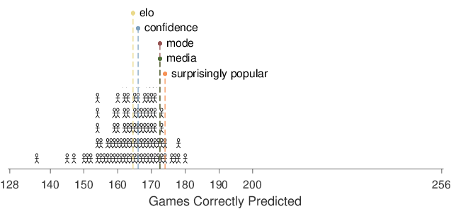
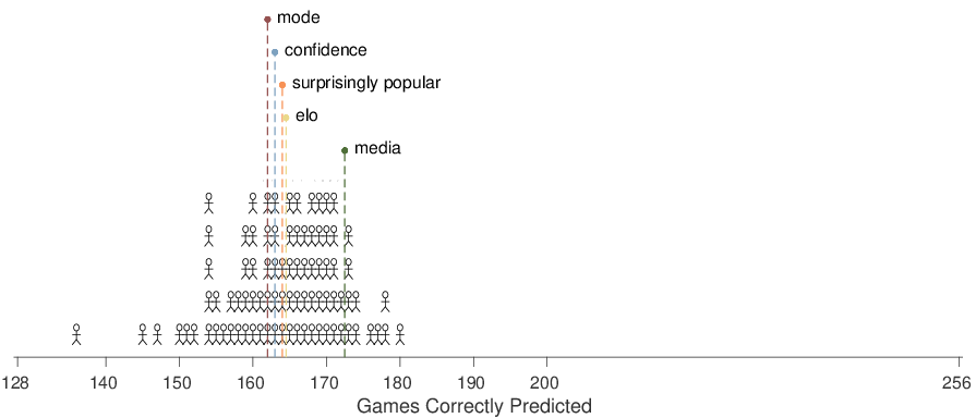
| Figure 3: The number of games correctly predicted by the surprising popular (sp), confidence-weighted tally (conf), mode of AMT participants (mode), mode of media experts (media), and Elo (elo) methods, and for 94 individual media experts. The stick figures represent the distribution of the number of games correctly predicted by the media experts. The labeled lines show the number of games correctly predicted by the methods. |
Given the goal of testing the ability of the surprisingly popular
method to make accurate predictions, it makes sense to focus on those
participants who are evidently supplying good predictions, calibrated
confidence judgments, and reasonable meta-cognitive estimates. Thus,
the following results focus exclusively on the AMT participants who
self-rated as “extremely knowledgeable” about the NFL. The ideal
experimental test of the surprisingly popular method would have been
to ask the media experts to provide meta-cognitive
judgments. Obviously, this was not possible, and so the group of AMT
participants who most closely match the media experts in terms of
prediction accuracy serves as a sensible surrogate group. The number
of “extremely knowledgeable” AMT participants varied from week to
week, from a minimum of 12 participants, to a maximum of 33
participants, with a mean of 18 participants.
It is worth noting that the basis for identifying this group is
self-rating data that were available before the games were
played, and so could form part of a real-world prediction method. We
emphasize, however, that there is an exploratory aspect to this method
of analysis. In particular, although we posted all of our raw data
before games were played, the analysis method was not
pre-registered. Thus, it is important to replicate our findings to
test the efficacy of self-rating in identifying accurate
participants. For completeness, in the supplementary information, we
present analyses of the surprisingly popular method based on all of
the AMT participants. In the on-line supplementary material, we also
provide the results of another variant suggested by a reviewer that
uses all but the least knowledgeable AMT participants. In both cases,
the prediction accuracy is much less impressive.
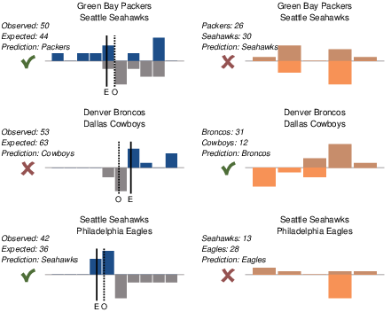
| Figure 4: Illustrative examples of the surprisingly popular and
confidence-weighted tally methods for three NFL games. The three
games correspond to the rows of panels, with the left-hand panel
corresponding to the surprisingly popular method, and the right-hand
panel corresponding to the confidence-weighted tally method. For the
surprisingly popular method, as in
Figure 1, the distributions of
meta-cognitive estimates of agreement are shown for people choosing
each team, and the observed and expected percentages of first-named
home-team prediction are detailed, along with the answer of the
method and its accuracy. For the confidence-weighted tally method,
the distributions of confidence on a 5-point scale are shown for
people choosing each team, and the confidence tallies are detailed,
along with the answer of the method and its accuracy. |
3.2 Accuracy of the Surprisingly Popular Method and Other Predictions
Figure 3 summarizes the overall performance
of the surprisingly popular method, in the context of the performance
of the individual media experts and other comparison methods. The
stick figures show the distribution of the total number of games in
the season correctly predicted by the 94 individual media experts. The
worst-performed experts correctly predicted the outcome of around 150
of the 256 games, the best-performed experts correctly predicted about
180 games, and most experts were correct for between 155 and 175 of
the games.
Note that, while the individual media experts made forced choices
between the two teams in a game, the aggregate methods can all produce
tied outcomes that favor neither team. The surprisingly popular method
can produce equal expert and observed percentages, although that never
happened for the current data. The confidence-weighted tallies can be
equal for both teams, which happened for five games. The number of
people favoring each team can be equal in determining a mode, which
happened for nine games for the AMT expert participants, and once for
the media experts. Finally, the Elo method can give a 50% winning
percentage to both teams, which occurred for five games. For these
games, the overall accuracies we report count these predictions as
half a game.
The surprisingly popular method, based on the group of AMT
participants self-rated as “extremely knowledgeable”, predicted 174
games correctly. This performance was inferior to five of the media
experts, the same as two more, and superior to the remaining 87. The
surprisingly popular method also slightly outperformed the modal (most
common) predictions of the “extremely knowledgeable” AMT
participants and the modal predictions of the media experts. These
mode-based predictions were both correct for 1721/2 of the
256 games. The confidence-weighted tally of the “extremely
knowledgeable” AMT made correct predictions for 166 games. These
predictions were based on the team with the larger sum of confidence
ratings across all of the participants favoring that team. The team
with the greater Elo predicted winning percentage was correct for
1641/2 games.
3.3 Examples of the Surprisingly Popular Method
Figure 4 presents three examples of the
performance of the surprisingly popular method, and the
confidence-weighted tally method, aimed at giving some insight into
the relative success of the surprisingly popular method. The detailed
results for every game are available in the supplementary
material. The three examples in Figure 4 were
chosen because the surprisingly popular and confidence-weighted tally
methods make different predictions and because, in two cases, the
surprisingly popular prediction does not follow the majority. It is
the ability of the surprisingly popular method to predict against
confidence-based and majority opinion that makes it theoretically
interesting.
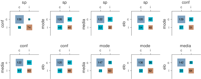
| Figure 5: Relationship between pairs of methods and the accuracy of
their predictions. Each panel corresponds to one of the 10 unique
pairings of the five methods: surprising popular (sp),
confidence-weighted tally (conf), mode of AMT participants (mode),
mode of media experts (media), and Elo (elo). Within each panel,
correct predictions are labeled as “c” and incorrect predictions
are labeled as “i”. The areas of squares and overlain numbers show
counts of games in which both methods made the same correct
prediction (top-left), the same incorrect prediction (bottom-right),
the left-labeled row method made a correct prediction but the
top-labeled column method did not (top-right), or the top-labeled
column method made a correct prediction but the left-labeled row
method did not (bottom-left) |
.
For each of the games in Figure 4 — between the
Green Bay Packers and Seattle Seahawks in week 1, the Denver Broncos
and Dallas Cowboys in week 2, and the Seattle Seahawks and
Philadelphia Eagles in week 15 — the surprisingly popular method is
shown on the left, and the confidence-weighted tally method is shown
on the right. The surprisingly popular method uses the same display
format used in Figure 1. The
confidence-weighted tally method is shown by histograms representing
the distribution of confidence ratings on the five-point scale. The
confidence distribution for predictions favoring the first-named team
is above and the confidence distribution for predictions favoring the
second-named team is below. The tally of these confidence ratings is
displayed as is the prediction made by the method.
In the Packers versus Seahawks game, the predictions of the
participants are evenly split between the two teams. The surprisingly
popular method predicts a Packers victory because many participants
favoring the Packers believe relatively few others will agree with
them. This means the relatively high percentage of participants
predicting a Packers victory is above the expectation. The confidence-weighted
tally method, however, predicts a Seahawks victory, because
participants favoring the Seahawks tended to do so with higher
confidence. This game provides a good example of the different
mechanisms by which these two methods break a 50–50 tie in the binary
predictions. As the tick and cross marks in
Figure 4 indicate, the winner of the game was the
Packers, and so the surprisingly popular method made the correct
prediction.
In the Broncos versus Cowboys game, the surprisingly popular method
chooses against the majority prediction. A total of 53% of
participants favored the Broncos, but many participants favoring the
Cowboys expected relatively few others to agree with them, leading to
a higher expectation of 63%. Thus, the observed percentage in favor
of the Broncos fell short of the expectation, and the “underdog”
Cowboys were predicted. Meanwhile, the confidence-weighted tally
method predicted a Broncos victory by some margin, since participants
favoring the Broncos generally expressed high confidence while
participants favoring the Cowboys generally expressed low
confidence. As it turned out, the Cowboys won the game, so the
confidence-weighted tally method made the correct prediction.
Finally, in the Seahawks versus Eagles game, there is an expectation
that the Eagles are heavy favorites. Most participants who predict an
Eagles win believe the majority of others will agree with them. Most
participants predicting a Seahawks win believe the majority will
disagree with them, but will instead favor the Eagles. Thus, even
though a minority of 42% of participants predicted the Seahawks to
win, this is higher than than the 26% expectation, and the
surprisingly popular method correctly predicts the eventual Seahawks
win.
3.4 Overlap in Predictions
Figure 5 provides a summary of the relationship between
the predictions of the different methods and their accuracies. The
panels correspond to all 10 possible pairings of the five aggregation
methods. Within each panel, a 2×2 table is shown counting how
often the pair of methods both made correct predictions, both made
incorrect predictions, or one method was correct and the other was
not. To measure these counts, we treated the tied predictions, in
which a method did not make a clear prediction, as errors. The left
column corresponds to correct predictions for the method labeled at
the top, and the top row corresponds to correct predictions for the
method labeled at the left. Within each cell, the area of the square
is proportional to how often the pattern of correct and incorrect
predictions across the pair of methods was observed, and the actual
count is also displayed.
The results in Figure 5 show that the surprisingly
popular method and the confidence-weighted tally method tend to
produce more similar predictions than other pairings of methods. The
two mode-based methods using expert judgments, for the AMT
participants and the media experts, are also quite similar in their
predictions. Meanwhile, the surprisingly popular method has the least
overlap in its predictions with those made by other data sources: the
media experts and the Elo method. Collectively, these results suggest
that both the data source and the aggregation method contribute to the
patterns of predictions.
Because the results show that the five methods have considerable
variety in their predictions, it is possible that further aggregation
across models could be useful. This is a familiar approach from
machine learning, known as boosting (Hastie et al., 2001), which
often leads to improved predictions. As it turns out, the modal
prediction of the five methods used in Figure 5 is
correct for 178 out of the 256 games, which is more accurate than any
of the individual methods. This result is obviously highly
exploratory, and needs to be replicated. It is also the case that the
five methods used were not chosen in an attempt to maximize the
accuracy of this type of aggregation, and it is possible that using
more or different methods would be a better approach.
3.5 Calibration
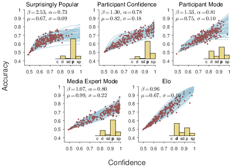
| Figure 6: Results of the calibration analysis for the five aggregation
methods. In each panel, the inset histogram shows the posterior
probability of the 5 possible logistic growth models (“c” =
chance, “d” = deterministic, “sd” = shifted deterministic, “p”
= probabilistic, “sp” = shifted probabilistic) used by
(LeeLee, 2017). The most likely model is labeled in
bold. The lines show samples from the posterior distribution of the
most likely calibration model, and the circular markers show samples
from the joint distribution of confidence and accuracy for the
predictions of the NFL games. |
Our final analysis considers the calibration of predictions made by the surprisingly popular and other methods. Ideally, a method would always make correct predictions, but, since errors are inevitable, it is important to know how much confidence should be placed in a prediction. Confidence guides decisions and actions that are made based on predictions, such as betting. We examine the calibration of each method in terms of a calibration curve that relates the confidence in predictions to their empirical accuracy (Lichtenstein et al., 1982).
For the Elo method, the confidence in a decision is given directly by the winning probabilities it produces. For the methods based on the majority prediction across people, the proportion of people in the majority is a natural measure of confidence (Grofman et al., 1983,KerrTindale, 2004). For the confidence-weighed tally method, an obvious measure of confidence is the tally in favor of the team predicted to win, expressed as a proportion of the sum of both tallies. For example, in the Houston Texans versus Tennessee Titans game in the top-right panel of Figure 4, the Titans are predicted to win, since their tally of 27 is greater than 22. The confidence in this prediction, according to the measure we use, is 27/(27+22)≈ 55%. For the surprisingly popular method, one possible way to measure confidence is the difference between the expected and observed percentages for a team, since it is this difference that determines the prediction. We add this difference to the chance probability of 50% to determine the confidence the surprisingly popular method has in each prediction it makes. For example, for the same Houston Texans versus Tennessee Titans game, the Texans are predicted to win, since the observed percentage of people predicting them to win is 47%, which is greater than the expected 45%. The confidence in this prediction, according to the measure we use, is 50+|47−45|= 52%.
To examine the calibration relationship between confidence and accuracy, we use the statistical approach developed by (LeeLee, 2017), which is summarized in the supplementary information. This approach infers calibration curves based on logistic growth functions. It aims first to infer what type of growth function best describes the calibration curve and then infers the parameters of the appropriate function. Both the type of curve and the parameters have meaningful psychological interpretations, which help to characterize and measure the calibration properties of a method. Figure 6 shows the results of the calibration analysis for the five methods. For each method, the inferred type of calibration curve is shown by the inset histogram. The curve relates the confidence a method has in a prediction on the x-axis to the probability the prediction is correct on the y-axis. The inferred posterior distribution for the calibration curve is shown by the lines, with the posterior for individual predictions shown by circular markers.
The inferred parameters from the (LeeLee, 2017) analysis for each method are also shown in Figure 6. The parameter β measures how quickly additional confidence leads to more accurate predictions (i.e., the slope of the calibration curve); α measures the upper-bound on accuracy (i.e., how accurate decisions made with 100% confidence are expected to be); µ measures the mean level of confidence a method has across all of its predictions; and σ measures the standard deviation of the distribution of confidence. The Elo method stands out as being extremely well calibrated. It has a slope near β=1. It is inferred to be deterministic, meaning that in theory a 100% confident prediction will be 100% accurate. The mean level of confidence is about 67% and rarely are predictions made with more than 80% certainty. This caution contrasts with the high confidence of the media modal decision, which has a mean confidence of µ=0.99 but has an upper-bound on accuracy of α=0.80. The participant mode and confidence-weighted tally calibration curves fall somewhere between these extremes. Both show a broader distribution of confidence. They have similar upper bounds on accuracy to the media mode method.
It does not make sense to compare the calibration curve of the surprisingly popular method to the calibration curves of the other methods, even though the surprisingly popular method is our focus. While the difference between expected and observed proportions is the obvious way to generate a measure of confidence, it is not obvious how this difference should be scaled. The current scaling assumes a difference of 50% is maximal, which seems reasonable, but not the only possible choice. In addition, it is not obvious that the scaling should be linear, as is currently assumed. Theoretical development is needed to provide a strong test of the calibration properties of the surprisingly popular method. What the results in Figure 6 do suggest, however, is that the surprisingly popular method is at least capable of reasonable calibration, in the sense that increasing differences between the observed and expected agreement correspond to more accurate decisions.
4 Discussion
Our results suggest there is promise in applying the surprisingly popular method to predicting the outcomes of NFL games. The surprisingly popular method outperformed most of the media experts, the majority opinion of these experts, the Elo method, and other measures based on our AMT participant data. While the improvement in accuracy was small, the nflpickwatch.com and Elo measures provide genuine real-world benchmarks. If the current level of improvement was replicated for other seasons, it would be have implications for real-world prediction and betting.
Despite this promise, we recognize the limitations of evaluating of any prediction method based on only one season, comprising a few hundred binary outcomes. Accordingly, we view this study as a motivating demonstration of the applicability of the surprisingly popular method to making predictions, with a particular focus on the important class of predictions represented by sporting contests. It seems clear that people were able to make decisions and provide meta-cognitive judgments in a prediction setting as naturally as they are able in previously studied non-prediction settings like general knowledge questions. Indeed, as the examples in Figure 4 highlight, the basic insight of the surprisingly popular method can generalize to predictive settings. If a subset of people have insight into a surprise winner, the surprisingly popular method provides a simple and effective way to capture and use that knowledge.
The key question, therefore, is whether and how often such subsets of people exist. Our study provided some first suggestive evidence that they can exist and suggests that domain knowledge, as measured by self-rating in our case, may be an important factor. Future work should try and isolate the type of expertise, or the types of games, that are likely to have the private knowledge or insight needed. As we mentioned, the ideal test is how well the surprisingly popular method performs when media experts provide meta-cognitive estimates of agreement, without being aware of the predictions others are making.
Another direction for future research is suggested by the meta-cognitive judgments that are the novel empirical feature of the surprisingly popular method. It is clear from the illustrative examples in Figure 4 that the distributions of these meta-cognitive estimates are generally broad. Whether this arises because of a individual differences in opinion about the percentage, individual differences in the cognitive processes in the way in the estimates are generated, or both, is an interesting cognitive modeling question. Potentially, a model-based account of these data could be incorporated into the surprisingly popular method to improve the precision of the meta-cognitive estimates (McCoyPrelec, 2017). Ideally, differences due to the cognitive processes involved in meta-cognition could be “factored out”, leaving the key signal of expected agreement.
The surprisingly popular method is a clever and simple approach to combining people’s judgments to make accurate group decisions, based on the insight that meta-cognitive information is important. Our results suggest that it may be useful in forecasting applications involving genuine predictions, as an alternative or complementary method to more elaborate approaches like prediction markets (Silver, 2012). We hope that our results encourage the further investigation of the surprisingly popular method, both in terms of its real-world performance, and the cognitive modeling challenges it poses for understanding the relationship between choice and meta-cognition.
References
-
[Elo, 1978]
-
Elo, A. E. (1978).
The rating of chessplayers, past and present.
Arco.
- [Grofman et al., 1983]
-
Grofman, B., Owen, G., & Feld, S. L. (1983).
Thirteen theorems in search of the truth.
Theory and Decision, 15, 261–278.
- [Hastie et al., 2001]
-
Hastie, T., Tibshirani, R., & Friedman, J. (2001).
The Elements of Statistical Learning.
New York, NY: Springer Verlag.
- [KerrTindale, 2004]
-
Kerr, N. L. & Tindale, R. S. (2004).
Group performance and decision making.
Annual Review of Psychology, 55, 623–655.
- [LeeLee, 2017]
-
Lee, M. D. & Lee, M. N. (2017).
The relationship between crowd majority and accuracy for binary
decisions.
Judgment and Decision Making, 12, 328–343.
- [Lichtenstein et al., 1982]
-
Lichtenstein, S., Fischoff, B., & Phillips, L. D. (1982).
Calibration of probabilities: The state of the art to 1980.
In D. Kahneman, P. Slovic, & A. Tversky (Eds.), Judgment under
uncertainty: Heuristics and biases (pp. 306–334). Cambridge, England:
Cambridge University Press.
- [McCoyPrelec, 2017]
-
McCoy, J. & Prelec, D. (2017).
A statistical model for aggregating judgments by incorporating peer
predictions.
arXiv preprint arXiv:1703.04778.
- [Plummer, 2003]
-
Plummer, M. (2003).
JAGS: A program for analysis of Bayesian graphical models using
Gibbs sampling.
In K. Hornik, F. Leisch, & A. Zeileis (Eds.), Proceedings of
the 3rd International Workshop on Distributed Statistical Computing (DSC
2003).
- [Prelec et al., 2017]
-
Prelec, D., Seung, H. S., & McCoy, J. (2017).
A solution to the single-question crowd wisdom problem.
Nature, 541, 532–535.
- [Rouder et al., 2009]
-
Rouder, J. N., Speckman, P. L., Sun, D., Morey, R. D., & Iverson, G. (2009).
Bayesian t-tests for accepting and rejecting the null hypothesis.
Psychonomic Bulletin & Review, 16, 225–237.
- [Silver, 2012]
-
Silver, N. (2012).
The signal and the noise: Why so many predictions fail – but
some don’t.
Penguin.
- [TetlockGardner, 2016]
-
Tetlock, P. E. & Gardner, D. (2016).
Superforecasting: The art and science of prediction.
Random House.
| Figure 7: The number of games correctly predicted by the surprising popular (sp) , confidence-weighted tally (conf), mode of AMT participants (mode), based on all of the AMT participants. The number of games correctly predicted by the mode of media experts (media) and Elo (elo) methods, and for 94 individual media experts, are shown. |

| Figure 8: The accuracy of the predictions made by the surprising popular (sp), confidence-weighted tally (conf), mode of AMT participants (mode), mode of media experts (media), and Elo (elo) methods, for every game of the NFL season. Panels correspond to weeks of the seasons, rows to methods, and columns to games. Dark blue circles indicate a correct prediction; light orange circles indicate an incorrect prediction; and grey circles indicate neither team was favored. |
Supplementary Information
Results For All AMT Participants
Our application of the surprisingly popular method relies on just those AMT participants who self-rated as being “extremely knowledgeable” about NFL football. The rationale for limiting the analysis to these participants is to use them as surrogate experts, from whom the meta-cognitive estimation of agreement was available. It is natural, however, also to consider the performance of the surprisingly popular method based on all of the available AMT participants. These results are summarized in Figure 7. It is clear the surprisingly popular method performs much more poorly, with an accuracy well below the mode of the media experts, and in the middle of the distribution of the individual accuracies for these experts. Presumably, this decrease in accuracy is the result of the less accurate judgments made by the non-expert AMT participants, as evident in the left-hand panels of Figure 2.
All Predictions
Figure 8 details the accuracy of every aggregate prediction method for every game. Each panel corresponds to a week, labeled “w1” for week 1, and so on. Within each panel, rows correspond to methods, and columns to games, ordered from left to right from best overall predicted to worst overall predicted. A dark blue circle indicates a correct prediction; a light orange circle indicates an incorrect prediction; a gray circle indicates neither team was favored by the method. Not surprisingly, there is often strong agreement across the methods. Most weeks include a number of games where all the methods make the same prediction: more often than not this prediction is correct, leading to a column of blue circles, but sometimes it is incorrect, leading to a column of orange circles.
Calibration Modeling
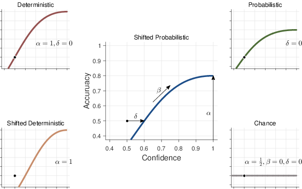
| Figure 9: Logistic growth calibration curves relating confidence on the x-axis to accuracy on the y-axis. The central panel shows the general model, with a growth parameter β, a bound parameter α, and a shift parameter δ. Surrounding panels show specific-case nested models with natural interpretations. Based on (LeeLee, 2017, Figure 3). |
Our calibration analysis is a natural extension of the approach developed by (LeeLee, 2017). Their approach applies directly only to the prediction methods based on the majority decision over a set of individuals, but can be generalized straightforwardly to include methods with other measures of decision confidence. Formally, in the (LeeLee, 2017) approach, there are n decisions, and the ith decision has ki people making the majority decision out of ni people, with an accuracy of yi=1 if the majority decision is correct, and yi=0 otherwise. The proportion θi represents the size of the majority and the probability φi representing the probability the decision correct.
This approach applies directly to the majority decisions based on AMT participants and media experts. The observed majority is assumed follows a binomial distribution with respect to the underlying majority proportion and the total number of people, so that ki ∼ Binomial(θi,ni). For the surprisingly popular, confidence-weighted tally, and Elo methods, which produce a continuous measure of confidence, ci for the ith decision, we assume this observed confidence reflects the underlying confidence with a small amount of noise, so that ci ∼ Gaussian(θi,1/(0.01)2). In both cases, the observed accuracy is a Bernoulli draw with respect to the underlying accuracy, yi ∼ Bernoulli(φi) and the distribution of confidence across all decisions is modeled as coming from an over-arching truncated Gaussian distribution, so that
θi ∼ Gaussian(0,1)(µ,1/σ2) where µ∼Uniform(1/2,1) and σ∼Uniform(0,1/2) are the mean and standard deviation, respectively.
To model the relationship between confidence and accuracy, (LeeLee, 2017) rely on a logistic growth model of the form
|
φi = α/ | ⎛
⎝ | 1+exp | ⎧
⎨
⎩ | −β | ⎡
⎣ | log | |
−log | |
− | | log | ⎛
⎝ | 2α−1 | ⎞
⎠ | ⎤
⎦ | ⎫
⎬
⎭ | ⎞
⎠ |
(1) |
with a growth parameter β, a bound parameter α, and a shift parameter δ. This model is shown in the central panel of Figure 9. The upper bound on accuracy is controlled by α. As the confidence in a decision increases, its accuracy increases at a rate controlled by β, with β=1 corresponding to a linear increase, values β>1 corresponding to faster increases, and values β<1 corresponding to slower increases. In the limit β=0, there is no growth in accuracy. The shift of the growth curve is controlled by δ. When δ=0 a decision made with no confidence has chance accuracy.
(LeeLee, 2017) also consider four special cases of the full shifted probabilistic model, shown in the surrounding panels of Figure 9. The deterministic model in the top-left corresponds to setting δ=0, α=1, and allowing only β to vary. The deterministic shift model in the bottom-left corresponds to setting just α=1, allowing for worse-than-chance performance. The probabilistic model in the top-right corresponds sets δ=0 so that accuracy starts at chance and grows to some upper bound α as confidence increases. Conceptually, α corresponds to the upper bound measuring the inherent (un)predictability of the domain, and β corresponds to how quickly that limit is approached. Finally, the chance model in the bottom-right corresponds to setting α=1/2, β=0, and δ=0, which reduces the model to θ=1/2 for all levels of confidence, so that accuracy is always at chance.
We follow (LeeLee, 2017) by implementing this model as a graphical model in JAGS (Plummer, 2003), which allows for fully Bayesian inference using computational sampling methods. The full shifted probabilistic model, and its four special cases, are treated as components of a latent-mixture model, allowing both the type of calibration curve and its parameters to be inferred.
This document was translated from LATEX by
HEVEA.