Judgment and Decision Making, Vol. 13, No. 5, September 2018, pp. 471-483
Time-varying risk behavior and prior investment outcomes: |
Risk behavior can be capricious and may vary from month to month. We study 62 clients of a private bank in Northern Italy. The individuals are of special interest for several reasons. As active traders, they manage the value-at-risk (VaR) of a portion of their wealth portfolios. In addition, they act alone, i.e., without input from a financial adviser. Based on VaR-statistics, we find that, in general, the subjects become more risk-averse after suffering losses and more risk-seeking after experiencing gains. The monthly gains and losses that alter investor risk behavior represent true changes in wealth but are “on paper” only, i.e., not immediately realized. Our results allow several interpretations, but they are not at odds with a house money effect, or the possibility that overconfident investors trade on illusions. Rapidly shifting risk behavior in fast response to unstable circumstances weakens individual risk tolerance as a deep parameter and key construct of finance theory.
Keywords: risk attitude, gains perception, losses perception, decision making
“There are two times in a man’s life when he should not speculate. When he can’t afford it, and when he can.” Mark Twain, Pudd’nhead Wilson’s New Calendar, 1897
Speculative gambling is risky business. While Mark Twain counsels against investment bets, no matter what, his words admit that people’s changing fortunes often have a bearing on what they decide to do.
Understanding how prior gains and losses affect risk attitudes is a significant question in the study of intertemporal choice. Research in this field has produced various perplexing results. Some experimental studies suggest that individuals often become more willing to gamble following gains (Thaler & Johnson, 1990). Other studies propose either that individuals become more risk-seeking after losses (Langer & Weber, 2008) or, the opposite, more risk-averse (Shiv et al., 2005; Liu et al., 2010).1 Here, we investigate the degree to which the experience of gains and losses influences subsequent asset allocation choices made by a sample of clients of an Italian private bank. Thus, we look at the risk behavior of real-world investors, the paper gains or losses in their portfolios, and their monthly asset allocation changes during the year 2015.2
As it happens, supervisory authorities in Italy and elsewhere require banks and other financial intermediaries to identify the risk profile of each client — commonly on a scale that runs between “no-risk” and “risk-seeking”. The level of hazard assumed by an investor’s portfolio is supposed to correspond to his or her risk profile. This is why financial service firms assess a value-at-risk (VaR) measure which determines the maximum amount of potential loss and its probability within a specific time frame. Banks and financial intermediaries gather information about clients through forms approved by supervisory authorities. The questionnaires list demographic and financial characteristics such as age, gender, level of education, work experience, financial knowledge and wealth. These characteristics determine the level of VaR that is suitable for a given investor.3 Banks and financial intermediaries must check whether the VaR of a particular portfolio matches its owner’s risk profile. The portfolio VaR fluctuates over time as an investor modifies his or her asset allocation, but it can never be allowed to exceed the investor’s VaR.
We examine monthly asset allocation changes made by clients of an Italian private bank. The bank in question considers six levels of VaR: 0 represents “no-risk”; 1, “low-risk”; 2, “prudent balanced risk”; 3, “balanced risk”; 4, “aggressive balanced risk”; and 5 “high-risk”. The greater the loss a specific investor is able to tolerate, the higher the VaR is permitted to be. To repeat, VaR itself assesses the level of risk of the portfolio. This aspect of our study is noteworthy since — as far as we know, without exception — past empirical research on investor trading assesses only the risks and returns associated with individual transactions.
Portfolio allocation decisions are often altered by an investor’s advisor (see, e.g., Foerster et al., 2017). Evidently, the fact that advisors guide investors makes it difficult to interpret the findings of an analysis like the one already outlined. That is why we opt for a much smaller sample comprised only of investors who act on their own (i.e., without experienced advisors) and who all qualify for the highest level of VaR.
Our paper contributes to the literature on dynamic choice under risk and uncertainty. How do past gains and/or losses influence the level of downside risk assumed by investors? Section ?? summarizes past research and “what we know” about risk behavior. Sections ?? presents our data collection effort. Section ?? presents the main hypothesis and the methods that are used. Section ?? discusses the results. Section ?? concludes.
A central feature of prospect theory and its successor, cumulative prospect theory, is that people are not consistently risk-averse (Kahneman & Tversky, 1979; Tversky & Kahneman, 1981; Tversky & Kahneman, 1992). Rather, people are risk-seeking in the domain of losses and risk-averse in the domain of gains, with gains and losses defined relative to a target or reference point. Also, individuals feel the pain of a loss more acutely than the pleasure of an equal-sized gain. These basic insights are corroborated by many experimental studies of risky decision making.4 Kahneman even dismisses as a “myth” the widespread belief among finance experts that the task of an advisor is to find a portfolio that fits the investor’s attitude to risk. The fundamental problem with individual risk tolerance, Kahneman submits, is that “there is no such thing” (2009, p. 1).5
Thaler and Johnson (1990) demonstrate that people tend to assume higher risk immediately following a previous gain. This psychological tendency is labeled the house money effect. It is supported by the further laboratory experiments of Battalio et al. (1990), Keasey and Moon (1996), and Ackert et al. (2006). Franken et al. (2006) study the Iowa Gambling Task of Bechara et al. (2000), which involves repeated choices among four decks of cards, two of which have negative expected value because they lead to large but infrequent losses. Young adults who experienced gains make more gainful and safer choices afterward than people who were subjected to losses. Then again, in an adaptation of Franken et al., Rosi et al. (2016) find that previous episodes makes no difference. As mentioned, Imas (2016) shows that many individuals with paper losses accept more risk but that, once a loss is realized, they take less risk. Imas also replicates selected findings of Shiv et al. (2005), Weber and Zuchel (2005), and Langer and Weber (2008).
Besides theory and laboratory-type experiments, there is limited empirical evidence. However, Malmendier and Nagel (2011) and Bucciol and Zarri (2015) look at the long-lasting effects on risk attitudes of traumatic experiences such as the Great Depression. Weber et al. (2012) use repeated surveys of British investors to study their risk taking during (and closely after) the 2008 financial crisis. Frino et al. (2008) consider the behavior of futures traders in Australia. Liu et al. (2010) look at market-makers in the Taiwan Futures Exchange. Gains earned during morning hours appear to produce above average risk-taking during afternoon trading. In addition, Hsu and Chow (2013) study individual investors in Taiwan. After substantial gains, investors assume greater risks. Hsu and Chow notice that, as time goes by, the house money effect slowly weakens. Lastly, Lien and Zheng (2015) look at slot machinge gambling.6
Clearly, it is difficult to tell what defines a gain or loss for a specific investor or to predict frames (Fischhoff, 1983; Barberis, 2013). For instance, investors may consider gains and losses in overall wealth, or in the value of their securities, or in the value of a certain asset. If we focus on a specific stock, a return that is positive may be considered a gain, or a return that exceeds the risk-free rate. Timing poses a further problem. Does the investor fixate on weekly, monthly, annual or lifetime gains and losses? This is the problem of choice bracketing Broad bracketing, which allows people to con¬sider all the consequences of their actions, often leads to superior decisions (Read et al., 1999).
Numerous studies attempt to connect risk preferences with demographic factors such as age, gender and education.7 As a rule, risk tolerance strengthens with a higher level of schooling, e.g., a university education (Riley & Chow, 1992; Halek & Eisenhauer, 2001; Hartog et al., 2002; Dwyer et al., 2002).
Generally, women are more risk-averse (e.g., Bajtelsmit & Bernasek, 1996; Powell & Ansic, 1997; Byrnes et al., 1999; Schubert et al., 1999; Eckel & Grossman, 2008; Lusardi & Mitchell, 2008; Croson & Gneezy, 2009) while men are more overconfident than women (e.g., Barber & Odean, 2000; Croson & Gneezy, 2009; Eckel & Grossman, 2008).
With respect to age, the evidence is more ambiguous. For example, Mikels and Reed (2009), Nielsen et al. (2008), and Albert and Duffy (2012) find that, compared to young adults, the elderly are more risk-averse for losses. Lauriola and Levin (2001), and Weller et al. (2011) indicate that the same is true for gains. On the other hand, Mather et al. (2012) suggest that aging instigates risk-seeking in the domain of losses, and Samanez-Larkin et al. (2007) and Thomas and Millar (2012) find no link, either for losses or gains, between risk attitudes and growing older. If measured by the ratio of risky assets to total wealth, risk tolerance may rise with age (Wang & Hanna, 1997). Regarding the link between age and the fraction of equity in investment portfolios (“the risky share”), there is no consensus.8
As a final point, we note that past gains and losses may also guide financial decisions for the reason that they change people’s beliefs, e.g., about their power to generate precise return forecasts or to control risk. Moore & Healy (2008) discuss various aspects of overconfidence. The experiments of Nosić & Weber (2010) imply that poor calibration encourages aggressive risk-taking. Merkle (2017) reports related empirical findings.9 Clearly, outcomes that validate a person’s beliefs or actions elevate confidence. People may fantasize that success primarily reflects personal ability. Self-assessments of competence correlate with self-assurance (Graham et al., 2009). That many people hold inflated views of themselves, and are also unaware of it (Kruger & Dunning (1999).
A private bank provided us with access to data. We are not allowed to disclose its name, but we can reveal that the bank is located in Northern Italy and that it is one of the five market leaders in financial planning, operating across Italy through a network of more than 1,000 financial advisers. As shown on http://www.assoreti.it, the website of the Associazione delle Società per la Consulenza agli Investimenti, the customers of banks such as ours typically have portfolios invested primarily, if not exclusively, in mutual funds, managed portfolios, insurance and pension funds. A fraction of clients, about 1 percent, use a part of their portfolio, usually between 5% and 10%, for direct investment in shares and/or bonds. With reference to this portion of the portfolio, managed autonomously, some clients adopt a buy-and-hold approach, i.e., they buy securities and hold them over extended periods of time. Others perform trading operations.
We created a data set using several criteria. First, we only consider investors with a total portfolio at the bank worth, on average, about €300,000 and with a portfolio that has two parts. The first piece, representing roughly 90% of its value, is administered with the supervision of a personal financial adviser. The second piece, corresponding to roughly 10%, is managed by the investor on his/her own via home banking. We label this part the “trading portfolio”. It is the main object of our study. Second, we study investors’ asset allocation decisions related to their trading portfolios during the calendar year 2015. In particular, we analyze data for clients who adjust their trading portfolios — at least once a month — but do not refashion the overall strategy of the total portfolio during 2015. This element is essential since, in some cases, financial advisers suggest specific asset allocation modifications, and clients may well apply the advice to their trading portfolios. To repeat, in order to be able to observe portfolio revisions made by clients in complete autonomy, we include only investors who never alter the asset allocation of the total portfolio under management but who do modify the trading portfolio.
Third, we exclude bank clients who add or withdraw funds (say, for consumption purposes) from their trading portfolio between January and December 2015. This makes it much easier for them to calculate and to mentally grasp monthly percentage returns and monetary gains or losses (in Euro).
Finally, we exclude clients who, for whatever reason, are not permitted by bank rules and procedures to raise their portfolio VaR into category 5, i.e., the maximum. Overall, our panel data set comprises data for 62 investors. For each, we have statistics regarding age, gender, level of education, the value of the trading portfolio, monthly gains and losses, and variations in portfolio risk exposure, i.e., the private bank’s estimates of the VaR of the trading portfolio. Our data are snapshots of portfolio value and VaR at the end of each month between January and December 2015.10 We note that the subjects in the sample have access to the same information and, of course, much more. On a bank website, they can inspect the composition of their trading portfolio, the account balance, and the VaR at any time, and as often as they wish. (The VaR is calculated around-the-clock.)11
Monthly changes in VaR are the dependent variable in the analysis that follows. In effect, we pretend that, at every month’s end, each individual subject faces a “decision point” where the performance of the trading portfolio over the most recent month is evaluated. At that time, the investor may resolve to vigorously correct the strategy. Only substantial adjustments would lead to a category change in VaR that becomes detectible, straightaway, over the current month. The main predictors of Δ VaR that we employ below are either a gain/loss dummy variable for changes in value of the trading portfolio during the prior month (priorGLD) (gain=1) or the percentage portfolio return (multiplied by 100) for the prior month (priorRET).
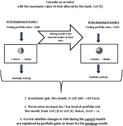
To be fully clear, consider an investor who at the beginning of month #1 has a trading portfolio of €100 (V1) invested in stocks and bonds with a VaR equal to 3. During the month, the investor performs at least one transaction that may modify the asset allocation within the trading portfolio and may produce a gain or a loss. Imagine that at the end of month #1 (which is also the start of month #2), the trading portfolio asset allocation is changed in terms of stocks and bonds so as to achieve a VaR equal to 4 and the value of the portfolio value is now €110 (V2). In this example, the investor obtains a gain of V2−V1 and records an increase in VaR from 3 to 4, so that the Δ VaR is +1. See Figure 1.
The main hypothesis tested below is that paper investment gains that are earned over an initial period embolden individuals to accept more risk during a later period. Conversely, current paper losses cause people to diminish risk afterward. We check whether changes in the VaR-category of the trading portfolio during month t (Δ VaR) are predicted by investor-specific portfolio gains or losses during month t−1.12
At first glance, the hypothesis appears to challenge prospect theory since we propose that achievement promotes adventure and failure invites prudence. This is false. We relate present changes in risk behavior (observed through fluctuations in VaR) to past returns. The time dynamics are key. Vis-à-vis decision-making under risk, not only future risk and return matter to investors, but so does history.
Our customized data set and empirical methods intend to reproduce a natural experiment, i.e., a study in which nature, i.e., factors outside our control, exposes clusters of individuals to dissimilar experimental and control conditions. Importantly, the process that governs exposures resembles random assignment. To repeat, we have access to portfolio values and VaRs at the end of each month between January and December 2015. This makes 62 investors ×11 months = 682 observations of Δ VaR, priorGLD, and priorRET. Since we relate changes in risk to prior month returns, the first set of 62 Δ VaRs that may be analyzed are for March 2015. The last set is for December 2015. All in all, we are able to examine investor behavior at 620 decision points which occur at the end of February 2015 through the end of November 2015 as subjects come to grips with the monthly performance of their trading portfolios.13
Since we have panel data, we estimate random-effects ordered logit regressions with changes in portfolio risk levels (Δ VaR) as a categorical dependent variable.14 Age, gender, education, and the total value of the trading portfolio at the end of the previous month serve as control variables. The main regression is:
|
Likewise, we run the same regression with priorGLD substituting for priorRET. We also conduct a string of robustness tests.
The main result is that, as hypothesized, the subjects become more risk-averse after suffering losses and more risk-seeking after experiencing gains, from month to month. Relevant details for this result are in Section 5.2. Section 5.1 provides basic descriptive statistics.
Tables ??, ?? and ?? offer descriptive statistics for 62 private bank clients. Hereafter, we briefly state — and further illustrate — the main facts in these tables.
Table 1: Descriptive statistics for 62 private bank clients. Panel A describes bank client age (in years), the value of the trading portfolio (Value, average of 12 monthly observations, in Euro), the change in portfolio value between end January and end December 2015 (ΔValue), and the value-at-risk category (1 to 5). Panel B shows means for subsamples of (1) men (M) and women (F), individuals (2) who are standard- or high-educated (LE and HE), (3) young or old, relative to the median sample age (Y and O), and hold (3) small or large trading portfolios, relative to the value of the median portfolio (SM and LG). We run t-tests for differences in means and Mann-Whitney U tests. The null hypothesis is that the sample means are equal. * (**) indicates statistical significance at the 5 (1) % level for t-tests; + (++) does the same for nonparametric tests.
Panel A: Full sample (62 observations) Age Value ΔValue VaR
Panel B: Subsamples Gender Education Age Portfolio value Obs. M(46) F(16) LE(35) HE(27) Y(31) O(31) SM(31) LG(31) Age 47.6 44.6 49.3 43.7 ** + 40.2 53.5 ** ++ 48.1 45.6 Value 32,001 27,935 * + 29,743 32,518 32,122 29,789 25,269 36,634 ** ++ ΔValue −118 13 −649 647 −344 174 −281 112 VaR 3.08 2.39 ** ++ 2.77 3.08 3.09 2.72 * 2.70 3.10 * +
Table 2: Pearson pairwise correlations, calculated for the 620 observations that correspond to the ordered logistic regressions estimated later in Table ??. Variables are measured monthly (at the end of month t) except Value, priorGLD and priorRET which are measured with respect to month t−1. Δ VaR is the portfolio value-at-risk category (1 through 5, with 5 indicating high risk) at the end of current month minus the value-at-risk at the beginning of the current month. VaR is the value-at-risk at the end of the current month. Age is measured in years. Gender is a dummy variable (female=1) and so is Education (high education=1). Value denotes portfolio value (in Euros) at the end of the previous month (which is the start of the current month). priorGLD is a dummy variable equal to one if the portfolio gained in value during the previous month. priorRET denotes the portfolio return during the previous month. RET is the portfolio return during the current month.
Δ VaR Age Gender Education Value priorGLD priorRET RET Age -0.025 1 Gender -0.015 -0.159 1 Education -0.002 -0.332 0.082 1 Value -0.059 -0.114 -0.247 0.186 1 priorGLD 0.200 -0.007 0.003 -0.033 0.117 1 priorRET 0.183 -0.016 -0.001 0.034 0.166 0.656 1 RET 0.440 -0.006 0.001 0.030 -0.125 0.217 0.286 1 VaR 0.250 -0.230 -0.376 0.191 0.319 0.183 0.200 0.112
The mean VaR across 682 monthly observations was 2.90. The 2015 age of the individuals in the sample varied between 35 and 65 years. On average, the subjects were 47 years old. Sixteen (26%) were women; 44% were university-educated. (Women were equally distributed between education levels.)
The mean trading portfolio balance, across investors and months, was €30,952. The minimum was €20,204 (investor #14, female, with a high-school education, age 55, and an average monthly VaR of 2.00) while the maximum was €46,125 (#25, male, high-school educated, 57, VaR 3.00).
The largest recorded loss in portfolio value between January and December 2015 was €13,000 (an 11-month return of −38.2% for #37, male, high-school educated, 41, VaR 2.92); the largest recorded gain came to €9,000 (a return of 32.1% for #33, female, university-educated, 40, VaR 2.42). The median investor lost €150.
Table 3: Portfolio VaRs, values, gains and losses, by month. Panel A shows VaRs by month, averaged across 62 subjects; the monthly fraction of subjects who raise or cut VaR; monthly cross-sectional averages of portfolio values, and of the ratios of the smallest and the largest portfolios relative to the mean portfolio. Panel B shows mean, minimum and maximum returns by month (in percent). In addition, it lists the fraction of all portfolios that rise in value during the month; the average gain or loss (in Euros) across all portfolios; and the matching monthly cross-sectional average of the absolute changes in value (in Euros).
Value of portfolios (in Euros) Panel A Mean VaR Δ VaR%+ Δ VaR %− Mean Min/Mean Max/Mean January 2.71 na na 29,181 0.69 1.44 February 2.74 0.03 0.00 30,364 0.66 1.47 March 2.89 0.16 0.02 31,089 0.65 1.48 April 3.05 0.18 0.02 31,931 0.62 1.50 May 3.18 0.15 0.02 32,820 0.62 1.51 June 3.15 0.05 0.08 33,541 0.61 1.52 July 3.19 0.05 0.00 33,887 0.60 1.53 August 3.13 0.02 0.08 33,192 0.62 1.63 September 2.76 0.00 0.34 29,573 0.61 1.45 October 2.65 0.03 0.15 28,281 0.62 1.45 November 2.65 0.03 0.03 28,463 0.63 1.44 December 2.76 0.15 0.03 29,096 0.64 1.45 ALL 2.90 0.08 0.07 30,952 0.57 1.74 Panel B Portfolio returns (in %) Portfolio gains or losses (in Euros) Mean Minimum Maximum % gains Aver. Aver. abs. February 3.75 -2.36 13.04 0.94 1,184 1,258 March 2.24 -4.26 9.93 0.84 725 973 April 2.31 -3.46 10.89 0.76 842 1,034 May 2.47 -6.90 16.51 0.76 889 1,163 June 2.11 -6.19 12.50 0.76 721 1,014 July 0.87 -7.00 9.38 0.73 346 730 August -2.51 -30.95 9.75 0.55 -695 1,618 September -12.20 -69.57 1.82 0.08 -3,620 3,675 October -4.76 -22.22 5.41 0.19 -1,292 1,553 November 0.61 -8.70 10.26 0.69 182 734 December 2.09 -9.52 13.33 0.89 633 778 ALL -0.29 -69.57 16.51 0.65 -8 1,321
Panel B in Table ?? shows data similar to panel A but for subsamples arranged by age, gender, education, and the monthly average trading portfolio balance. On average, older investors ran portfolios with somewhat lower VaRs but the difference is not large. Compared to the men, the women in the sample managed portfolios that were about €4,000 smaller with VaRs that were much lower. (Note the t- and Mann-Whitney U-tests.) Subjects with a university degree were on average 5½ years younger than high-school graduates. Larger portfolios displayed higher VaRs.
Some of the relationships thus far discussed are also visible in Table ??, a correlation matrix.
It shows that the current monthly returns earned by individual investors (RET), these same returns for the previous month (measured either by priorRET and priorGLD, the gain/loss dummy), the VaRs and Δ VaRs are all strongly positively correlated.
Table ?? shows some of the data month-by-month.
Between January and August 2015, the average portfolio was rising in value. This was followed by big negative shocks in September and October. The same pattern emerges in the monthly VaRs, averaged across bank clients. Also, in all months but September, there were some subjects who increased the value-at-risk of their portfolios; in all months but July, some decreased VaR. About 2/3’s of all monthly observations are gains; 8% are associated with increases in Δ VaR, 7% with decreases in Δ VaR, and 85% cause no change in value-at-risk.
Table 4: Monthly transitions between VaR categories. Panel A shows frequencies for 25 different types of VaR transitions as well as the number of of portfolio gains and losses (over the previous month) associated with specific VaR transitions (during the current month). In total, there are 620 decision points that lead to 98 VaR transitions to a different category. Panel B lists equivalent percentages totaling to 100 percent. Panel C shows the average Euro gain or loss for all transitions of a given type.
VaR category at the end of the month Panel A: of VaR transitions with gains or losses over the prior month Panel B: Fraction of VaR transitions (total = 100%) Panel C: Average gain or loss over the prior month (in Euros)
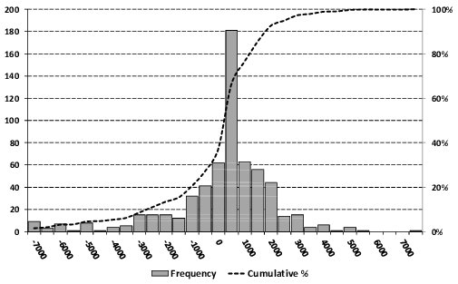
The simple average monthly portfolio return was minus 29 basis points, equivalent to a loss of €8. In terms of this investigation, the averages are deceptive, however. The absolute monthly change in portfolio value, averaged across individuals, is €1,321; the same statistic calculated for two-month periods is €2,294, and it is €3,202 for three-month periods. Figure 2 is a histogram with all one-month gains and losses for all subjects between February to November 2015. Evidently, most monthly value changes are modest, and cannot be expected to prompt changes in risk-taking, but a considerable number are very large relative to the size of the portfolio. As seen in Table ??, the cruelest monthly shock was a loss of €16,000 in September (−69.57% for #28, female, 41, high-school educated, VaR 2.83); the best result was a gain of €7,100 in May (+16.51% for #1, male, 35, university-educated, VaR 4.50).
In a simple analysis, we regressed the change in VaR category on whether the previous month showed a gain or a loss, for each subject. Of the regression coefficients, 39 were positive, 2 were negative, and 21 were 0. This difference suggests that changes of the last month affect risk taking in the present month.
For a more complete analysis, Table ?? (panel A) presents the transition matrix describing the frequency with which investors move their portfolios from one VaR category to another.
Table 5: Which factors cause variation in Value-at-Risk? We estimate random-effect ordered logistic regressions. The dependent variable is Δ VaR. The predictor variables are Age (in years), Gender (female=1), Education (high education=1), the value of the portfolio at the beginning of the month (in thousands of Euros), a gain/loss dummy (PriorGLD, gain=1) for the change in portfolio value during the prior month, and the portfolio return during the prior month (PriorRET, in percent). The regressions are for the full sample and for subsamples. *** is p<.01; **, p<.05; *, p<.10. S.E., clustered by individual investor, are in parentheses.
Full sample Men Women Standard-educated Highly-educated Age -0.01^** -0.01^*** -0.01^* -0.01^* -0.03 -0.04 -0.02^** -0.02^** -0.00 -0.00 (0.006) (0.007) (0.007) (0.007) (0.028) (0.026) (0.008) (0.009) (0.010) (0.012) Gender -0.34^** -0.33^** -0.32^** -0.26^* -0.38 -0.44 (0.132) (0.148) (0.141) (0.152) (0.253) (0.278) Education 0.08 0.01 0.06 0.01 0.03 -0.12 (0.109) (0.117) (0.126) (0.142) (0.292) (0.269) Value -0.04^*** -0.04^*** -0.03^*** -0.04^*** -0.08^*** -0.07^* -0.03^*** -0.04^*** -0.05^*** -0.05^*** (0.010) (0.010) (0.010) (0.010) (0.041) (0.042) (0.012) (0.011) (0.019) (0.021) priorGLD 1.39^*** 1.42^*** 1.33^*** 1.31^*** 1.50^*** (0.260) (0.313) (0.487) (0.408) (0.320) priorRET 0.07^*** 0.10^*** 0.01 0.07^** 0.08^*** (0.021) (0.019) (0.018) (0.033) (0.020) cut-off 1 -7.02^*** -8.06^*** -6.41^*** -7.74^*** -5.61^*** -6.35^** -7.27^*** -8.31^*** -6.86^*** -7.80^*** (0.864) (0.916) (0.822) (0.963) (2.391) (2.291) (1.327) (1.430) (1.046) (1.039) cut-off 2 -3.75^*** -4.79^*** -3.45^*** -4.71^*** -0.04 -1.09 -4.04^*** -5.08^*** -3.55^*** -4.47^*** (0.501) (0.550) (0.451) (0.556) (2.398) (2.154) (0.646) (0.715) (0.726) (0.911) cut-off 3 1.59^*** 0.41 1.83^*** 0.60 1.55^* 0.41 1.52^* 0.43 (0.553) (0.554) (0.531) (0.557) (0.732) (0.730) (0.922) (0.873) Obs. 620 620 460 460 160 160 350 350 270 270 Wald χ2 48.6^*** 31.8^*** 33.6^*** 41.8^*** 21.4^*** 3.8 19.2^*** 17.4^*** 35.4^*** 28.1^***
Each cell lists the total number of cases, the number of cases associated with portfolio gains during the previous month, and the ones associated with losses during that month. Panel B shows the fraction of VaR transitions of different types, and panel C lists the matching average €gain or loss, averaged across all observations for the matrix cell.
Since the largest percentages are on the main diagonal of panel B, Table ?? indicates that investors tend to preserve the status-quo level of VaR. Values outside the diagonal and other than zero represent the changes in VaR which we want to explain. The average Δ VaR is close to zero, and this remains true even if we exclude the 85% of cases on the diagonal. Some individuals changed VaR as often as three or four times during 2015. Others never did.
The main insight derived from Table ?? is that VaR increases (from 2 to 3, from 3 to 4, and from 4 to 5) are allied with a high proportion of gains and high average €gains during the previous month. VaR decreases (from 3 to 2, from 4 to 3, and from 5 to 4) are coupled with a high proportion of losses and high average €losses.15 This agrees with our main hypothesis.
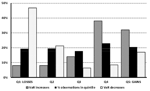
Figure 3 presents a different route to the same destination. There, all past one-month gains or losses, previously shown in Figure 2, are sorted into quintiles and, for each quintile, we find the fraction of all VaR increases and all VaR decreases associated with it. The results are crystal clear. Nearly half of all VaR decreases accompany the 20% of months with the worst portfolio performance. Also, roughly 70% of all VaR increases follow months with portfolio value changes in the top 40%. Lastly, the middle quintile shows less than proportional VaR increases and decreases. If past gains or losses did not bring about changes in risk-taking, all bars in Figure 3 should have been of the same height.
Table ?? displays the regression results for the full sample and various subsamples.
The cut-off points in the table are auxiliary parameters that separate the four categories of the dependent variable (Δ VaR) is +1, 0, −1, or −2). Equality tests strongly reject the null hypothesis that the cut-off points are equal — confirming the relevance of the four categories. For the sample as a whole, the results indicate that, except for education, all variables contribute in a significant way. The results are fairly uniform across subsamples.16 Older subjects are less likely to appear in the top category, i.e., their risk appetite is lower. The same applies to women, and to clients with somewhat more abundant portfolios.
In the financial industry, and also in finance theory, the assessment of investor risk profiles is normally seen as a elementary step toward identifying asset portfolios that are most appropriate to serve client needs. Past studies find that risk tolerance varies with demographic factors that change slowly over time or not at all. Here, we offer direct evidence that risk preferences and/or beliefs about one’s ability to manage risk and return evolve from month to month and in direct response to recent portfolio performance. This is shown for a sample of genuine investors who act on their own without external advisory influence. All told, fast-changing circumstances predict fast-changing risk attitudes.
If correct and characteristic of the behavior of important segments of the financial community, our empirical findings appear to offer some circuitous support for modern asset pricing theory in the manner of Campbell and Cochrane (1999) and others. The fact that we study active traders likely helps to explain why our results are so markedly different from the inertia reported by Brunnermeier and Nagel (2008) who, based on data from the Panel of Income Dynamics, report that most U.S. households do not adjust the share of their portfolios invested in risky assets following wealth changes, and who find in favor of constant relative risk aversion.17
Our chief result, however, is that, for the Italian bank clients in our sample, past portfolio performance — which, as we have seen, can be quite erratic — predicts short-term variations in risk-taking quantified by value at risk. The house money effect of Thaler and Johnson (1990) is not discarded by our data set, and neither is the alternate view that fluctuations in self-confidence, feeding an illusion of control, is the main culprit. However, the tests do appear to challenge Imas (2016).
The investors that we study are amateurs, not experts. Our analysis agrees with the Dunning-Kruger effect (Kruger & Dunning, 1999). Intuitively, it is plausible that amateurs look at past performance, even if not realized, to divine the future, especially when they act alone without highly trained assistance. Success builds confidence; failure undermines it.18 The switches from less risk tolerance to more, and vice versa, on the basis of near past performance also lead us straightforwardly to Bandura’s concept of self-efficacy. The beliefs that people hold about their capabilities, e.g., the presence or lack of mastery, affect the quality of their functioning. Self-efficacy has a bearing on thought patterns, emotional arousal, and behavior (Bandura, 1982). The findings in this article suggest to us that quite a few investors (i) may eventually come to doubt their own skills, (ii) may no longer put in much effort, and (iii) do not truly learn from experience. As their self-efficacy erodes, they may have a sense of futility, perhaps apathy.19 Of course, we recognize that these last sentences are highly speculative, and necessitate much more investigation. The results may also have some limited practical/regulatory use. Italian banks and financial intermediaries are required to monitor the level of risk of their clients’ portfolios so as to avoid excessive loss exposure and potential discontent. Financial advisers who observe unusual trading and fluctuations in risk-taking may use our findings for didactic purposes, leading clients to be more sensible in their investments and thereby also building more fruitful advisory relationships.
Ackert, L., Charupat, N., Church, B., & Deaves, R. (2006). An experimental examination of the house money effect in a multi-period setting. Experimental Economics, 9(1), 5–16.
Albert, S., & Duffy, J. (2012). Differences in risk aversion between young and older adults. Neuroscience and Neuroeconomics, 1, 3–9.
Andrade, E. B., & Iyer, G. (2009). Planned versus actual betting in sequential gambles. Journal of Marketing Research, 46(3), 372–383.
Arkes, H. R., Hirshleifer, D., Jiang, D., & Lim, S. (2008). Reference point adaptation: Tests in the domain of security trading. Organizational Behavior and Human Decision Processes, 105(1), 67–81.
Arkes, H. R., Joyner, C. A., Pezzo, M. V., Nash, J. G., Siegel-Jacobs, K., & Stone, E. (1994). The psychology of windfall gains. Organizational Behavior and Human Decision Processes, 59(3), 331–347.
Baetschmann, G., Staub, K. E., & Winkelmann, R. (2011). Consistent estimation of the fixed effects ordered logit model, Discussion Paper #5443, Forschungsinstitut zur Zukunft der Arbeit (www.econstor.eu).
Bajtelsmit, V., & Bernasek, A. (1996). Why do women invest differently than men? Financial Counseling and Planning, 7(1), 1–10.
Bandura, A. (1982). Self-efficacy mechanism in human agency. American Psychologist, 37(2), 112–147.
Barber, B., & Odean, T. (2000). Trading is hazardous to your wealth: The common stock investment performance of individual investors. Journal of Finance, 55(2), 773–806.
Barber, B., & Odean, T. (2001). Boys will be boys: Gender, overconfidence and common stock investment. Quarterly Journal of Economics, 116(1), 261–292.
Barberis, N. C. (2013). Thirty years of Prospect Theory in Economics: A review and assessment. Journal of Economic Perspective, 27(1), 173–196.
Battalio, R., Kagel, J., & Jiranyakul, K. (1990). Testing between alternative models of choice under uncertainty: Some initial results. Journal of Risk and Uncertainty, 3(1), 25–50.
Bechara, A., Tranel, D., & Damasio, H. (2000). Characterizations of the decision-making deficit of patients with ventromedial prefrontal cortext lesions. Brain, 123(11), 2189–2202.
Birnbaum, M. H. (2008). New paradoxes of risky decision making. Psychological Review, 115(2), 463–501.
Blume, M., & Friend, I. (1975). The asset structure of individual portfolios and some implications for utility functions. Journal of Finance, 30(2), 585–603.
Brunnermeier, M. K., & Nagel, S. (2008). Do wealth fluctuations generate time-varying risk aversion? Micro-evidence on individuals’ asset allocation. American Economic Review, 98(3), 713–736.
Bucciol, A., & Zarri, L. (2015). The shadow of the past: Financial risk taking and negative life events. Journal of Economic Psychology, 48, 1–16.
Byrnes, J., Miller, D., & Schafer, W. (1999). Gender differences in risk taking: A meta analysis. Psychological Bulletin, 125(3), 367–383.
Callen, M., Isaqzadeh, M, Long, D. J., & Sprenger, C. (2014). Violence and risk preference: Experimental evidence from Afghanistan. American Economic Review, 104(1), 123–148.
Cameron, L., & Shah, M. (2015). Risk-taking behavior in the wake of natural disasters. Journal of Human Resources, 50(2), 484–515.
Campbell, J. Y., & Cochrane, J. H. (1999). By force of habit: A consumption-based explanation of aggregate stock market behavior. Journal of Political Economy, 107(2), 205–251.
Caprara, G. V., Fida, R., Vecchione, M., Del Bove, G., Vecchio, G. M., Barbaranelli, C., & Bandura, A. (2008). Longitudinal analysis of the role of perceived self-efficacy for self-regulated learning in academic continuance and achievement. Journal of educational psychology, 100(3), 525–534.
Cardak, B., & Wilkins, R. (2009). The determinants of household risky asset holdings: Australian evidence on background risk and other factors. Journal of Banking and Finance, 33(5), 850–860.
Croson, R., & Gneezy, U. (2009). Gender differences in preferences. Journal of Economic Literature, 47(2), 448–474.
De Bondt, W. F. M. 1998. A portrait of the individual investor. European Economic review, 42(3–5), 831–844.
Dwyer, P. D., Gilkeson, J. H., & List, J. A. (2002). Gender differences in revealed risk taking: Evidence from mutual fund investors. Economics Letters, 76(2), 151–158.
Eckel, C., & Grossman, P. (2008). Forecasting risk attitudes: an experimental study using actual and forecast gamble choices. Journal of Economic Behavior and Organization, 68(1, 1–17.
Everson, H., & Tobias, S. (1998). The ability of estimate knowledge and performance in college: A metacognitive analysis. Instructional Science, 26(1–2), 65–79.
Fagereng, A., Gottlieb, C. & Guiso, L. (2013). Asset market participation and portfolio choice over the life-cycle. EUI Working Paper ECO 2013/07.
Fan, E., & Zhao, R. (2009). Health status and portfolio choice: Causality or heterogeneity? Journal of Banking and Finance, 33(6), 1079–1088.
Fischhoff, B. (1983). Predicting frames. Journal of Experimental Psychology: Learning, Memory, and Cognition, 9(1), 103–116.
Foerster, S., Linnainmaa, J. T., Melzer, B. T., & Previtero, A. (2017). Retail financial advice: Does one size fit all? Journal of Finance, 72(4), 1441–1482.
Franken, I., Georgieva, I., Muris, P., & Dijksterhuis, A. (2006). The rich get richer and the poor get poorer: On risk aversion in behavioral decision-making. Judgment and Decision Making, 1(2), 153–158.
Frino, A., Grant, J., & Johnstone, D. (2008). The house money effect and local traders on the Sydney Futures Exchange. Pacific-Basin Finance Journal, 16(1), 8–25.
Grable, J. E. (2008). Risk tolerance. In J. J. Xiao (Ed), Handbook of Consumer Finance Research (pp. 3–19). New York: Springer.
Graham, J., Campbell, R., & Hai, H. (2009). Investor competence, trading frequency, and home bias. Management Science, 55(7), 1094–1106.
Grinblatt, M., & Keloharju, M. (2009). Sensation seeking, overconfidence, and trading activity. Journal of Finance, 64(2), 549–578.
Guiso, L., Haliassos, M. & Jappelli, T. (2002), Household Portfolios. Cambridge, Massachusetts: The MIT Press.
Guiso, L., Sapienza, P. & Zingales, L. (2018). Time-varying risk aversion. Journal of Financial Economics, 128(3), 403–421.
Halek, M., & Eisenhauer, J. G. (2001). Demography of risk aversion. The Journal of Risk and Insurance, 68(1), 1–24.
Hartog, J., Ferrer-i-Carbonell, A., & Jonker, N. (2002). Linking measured risk aversion to individual characteristics. Kyklos, 55(1), 3–26.
Hinz, R., McCarthy, D., & Turner, J. (1997). Are women more conservative investors? Gender differences in participant-directed pension investments. In M. S. Gordon, O. S. Mitchell & M. M. Twinney (Eds.), Positioning Pensions for the Twenty-first Century (pp.45–66). Philadelphia: University of Pennsylvania Press.
Holton, G. A. (2014). Value-at-Risk: Theory and practice, e-book
at
urlhttp://value-at-risk.net (2nd ed.).
Hsu, Y. L., & Chow, E. (2013). The house money effect on investment risk taking: Evidence from Taiwan. Pacific-Basin Finance Journal, 21(1), 1102–1115.
Imas, A. (2016). The realization effect: Risk-taking after realized versus paper losses. American Economic Review, 106(8), 2086–2109.
Kahneman, D. (2009). The myth of risk attitudes. Journal of Portfolio Management, 36(1), 1–1.
Kahneman, D., Knetsch, J., & Thaler, R. H. (1991). The endowment effect, loss aversion, and status quo bias. Journal of Economic Perspectives, 5(1), 193–206.
Kahneman, D., & Tversky, A. (1979). Prospect theory: An analysis of decision under risk. Econometrica, 47(2), 263–291.
Kahneman, D., & Tversky, A. (1984). Choices, values and frames. American Psychologist, 39(4), 341–350.
Kaustia, M., & Knüpfer, S. (2008). Do investors overweight personal experience? Evidence from IPO subscriptions. Journal of Finance, 63(6), 2679–2702.
Keasey, K., & Moon, P. (1996). Gambling with the house money in capital expenditure decisions: An experimental analysis. Economics Letters, 50(1), 105–110.
Kruger, J., & Dunning, D. (1999). Unskilled and unaware of it: How difficulties in recognizing one’s own incompetence lead to inflated self-assessments. Journal of Personality and Social Psychology, 77(6), 1121–1134.
Langer, T., & Weber, M. (2008). Does commitment or feedback influence myopic loss aversion? Journal of Economic Behavior and Organization, 67(3–4), 810–819.
Lauriola, M., & Levin, I. (2001). Personality traits and risky decision-making in a controlled experimental task: An exploratory study. Personality and Individual Differences, 31(2), 215–226.
Lien, J. W., & Zheng, J. (2015). Deciding when to quit: Reference-dependence over slot machine outcomes, American Economic Review, 105(5), 366–370.
Liu, Y.-J., Tsai, C.-L., Wang, M.-C., & Zhu, N. (2010). Prior consequences and subsequent risk taking: New field evidence from the Taiwan Futures Exchange. Management Science, 56(4), 606–620.
Lusardi, A., & Mitchell, O. (2008). Planning and financial literacy: How do women fare? American Economic Review, 98(2), 413–417.
Malmendier, U., & Nagel, S. (2011). Depression babies: Do macroeconomic experiences affect risk taking? Quarterly Journal of Economics, 126(1), 373–416.
Mather, M., Mazar, N., Gorlick, M. A., Lighthall, N. R., Burgeno, J., Schoeke, A., & Ariely, D. (2012). Risk preferences and aging: The certainty effect in older adults’ decision making. Psychology and Aging, 27(4), 801–816.
Merkle, C. (2017). Financial overconfidence over time: Foresight, hindsight, and insight of investors. Journal of Banking & Finance, 84(C), 68–87.
Mikels, J., & Reed, A. (2009). Monetary losses do not loom large in later life: Age differences in the framing effect. Journal of Gerontology: Psychological Science and Social Science, 64B(4), 457–460.
Moore, D., & Healy, P. (2008). The trouble with overconfidence. Psychological Review, 115(2), 502–517.
Nielsen, L., Knutson, B., & Carstensen, L. (2008). Affect dynamics, affective forecasting, and aging. Emotion, 8(3), 318–330.
Nosić, A., & Weber, M. (2010). How riskily do I invest? The role of risk attitudes, risk perceptions, and overconfidence. Decision Analysis, 7(3), 282–301.
Novemsky, N., & Kahneman, D. (2005). The boundaries of loss aversion. Journal of Marketing Research, 42(2), 119–128.
Odean, T. (1999). Do investors trade too much? American Economic Review, 89(5), 1279–1298.
Poterba, J. M. & Samwick, A. A. (2001). Household portfolio allocation over the life cycle. In S. Ogura, T. Tachibanaki, & D. A. Wise (Eds.), Aging Issues in the United States and Japan (pp. 65–103). Chicago: University Of Chicago Press.
Powell, M., & Ansic, D. (1997). Gender differences in risk behaviour in financial decision-making. An experimental analysis. Journal of Economic Psychology, 18(6), 605–628.
Read, D., Lowenstein, G., & Rabin, M. (1999). Choice bracketing. Journal of Risk and Uncertainty, 19(1–3), 171–197.
Riley, W. B., & Chow, K. V. (1992). Asset allocation and individual risk aversion. Financial Analysts Journal, 48(6), 32–37.
Rosi, A., Cavallini, E., Gamboz, N., & Russo, R. (2016). On the generality of the effect of experiencing prior gains and losses on the Iowa Gambling Task: A study on young and old adults. Judgment and Decision Making, 11(2), 185–196.
Roszkowski, M. (2001). Risk tolerance in financial decisions. In D. M. Cordell (Ed.), Fundamentals of Financial Planning, 5th ed. (pp. 237–298). Bryn Mawr: The American College.
Samanez-Larkin, G., Gibbs, S., Khanna, K., Nilsen, L., Carstensen, L., & Knutson, B. (2007). Anticipation of monetary gain but not monetary loss in healthy older adults. Nature Neuroscience, 10(6), 787–791.
Schubert, R., Brown, M., Gysler, M., & Brachinger, H. (1999). Financial decision-making: Are women really more risk-averse? American Economic Review, 89(2), 381–385.
Shefrin, H., & M. Statman, M. (2000). Behavioral portfolio theory. Journal of Financial and Quantitative Analysis, 35(2), 127–151.
Shiv, B., Loewenstein, G., & Bechara, A. (2005). The dark side of emotion in decision-making: When individuals with decreased emotional reactions make more advantageous decisions. Cognitive Brain Research, 23(1), 85–92.
Shiv, B., Loewenstein, G., Bechara, A., Damasio, H., & Damasio A. R. (2005). Investment behavior and the negative side of emotion. Psychological Science, 16(6), 435–439.
Strahilevitz, M. A., Odean, T., & Barber, B. M. (2011). Once burned, twice shy: How naïve learning, counterfactuals, and regret affect the repurchase of stocks previously sold. Journal of Marketing Research, 48(SPL), S102–S120.
Thaler, R. H., & Johnson, E. J. (1990). Gambling with the house money and trying to break even: Effects of prior outcomes on risky choice. Management Science, 36(6), 643–660.
Thomas, A., & Millar, P. (2012). Reducing the framing effect in older and younger adults by encouraging analytical processing. Journal of Gerontology: Psychological Science and Social Science, 67B(2), 139–149.
Tversky, A., & Kahneman, D. (1981). The framing of decisions and the psychology of choice. Science, 211(4481), 453–458.
Tversky, A., & Kahneman, D. (1992). Advances in prospect theory: Cumulative representation of uncertainty. Journal of Risk and Uncertainty, 5(4), 297–323.
Wang, H., & Hanna, S. (1997). Does risk tolerance decrease with age? Financial Counseling and Planning, 8(2), 27–31.
Weber, M., & Zuchel, H. (2005). How do prior outcomes affect risk attitude? Comparing escalation of commitment and house-money effect. Decision Analysis, 2(1), 30–43.
Weber, M., Weber, E. U., & Nosic, A. (2013). Who takes risks when and why: Determinants of changes in investor risk taking. Review of Finance, 17, 847–883.
Weller, J., Levin, I., & Denburg, N. (2011). Trajectory of risky decision making for potential gains and losses for ages 5 to 85. Journal of Behavioral Decision Making, 24(4), 331–344.
Copyright: © 2018. The authors license this article under the terms of the Creative Commons Attribution 3.0 License.
This document was translated from LATEX by HEVEA.