Judgment and Decision Making, Vol. 16, No. 5, September 2021, pp. 1186-1220
Consumers’ ability to identify a surplus when returns to attributes are nonlinearPeter D. Lunn* Jason Somerville# |
Abstract:Previous research in multiple judgment domains has found that nonlinear functions are typically processed less accurately than linear ones. This empirical regularity has potential implications for consumer choice, given that nonlinear functions (e.g., diminishing returns) are commonplace. In two experimental studies we measured precision and bias in consumers’ ability to identify surpluses when returns to product attributes were nonlinear. We hypothesized that nonlinear functions would reduce precision and induce bias toward linearization of nonlinear relationships. Neither hypothesis was supported for monotonic nonlinearities. However, precision was greatly reduced for products with nonmonotonic attributes. Moreover, assessments of surplus were systematically and strongly biased, regardless of the shape of returns and despite feedback and incentives. The findings imply that consumers use a flexible but coarse mechanism to compare attributes against prices, with implications for the prevalence of costly mistakes.
Keywords: consumer choice, function learning, multiattribute decision making, nonlinear returns
The first 16 gigabytes of memory in a mobile device are more essential than a further 16 gigabytes. An initial 500 square feet of floor space in an apartment matter more than an additional 500 square feet. The ubiquity of such preferences means that theories of consumer decision making typically assume that preference functions have diminishing marginal returns to attributes. Thus, if consumers develop such preferences, they must process nonlinear functional forms to apply them.
Researchers in judgment and decision making have long been interested in nonlinear functional forms. (HammondSummers, 1965) argued that while linear regression might approximate the psychological process when an individual combines multiple cues to judge a quantity or probability, it is important to investigate how judgment copes when faced with a nonlinear relationship. Multiple experimental tasks have since compared performance when individuals try to combine linear and/or nonlinear cues to guess a quantity or category. These include inductive inference, multiple cue probability learning, function learning, and categorization. The evidence shows that individuals can take account of nonlinearity in functional relationships (HammondSummers, 1965,SummersHammond, 1966), but that judgments based on nonlinear functions are less accurate than those based on linear functions (Brehmer, 1971,Deane et al., 1972,BrehmerQvarnström, 1976,BrehmerSvensson, 1976,Brehmer, 1979,KarelaiaHogarth, 2008).
This previous work addressed settings where people aim to match real-world functional relationships, such as those between clinical results and medical diagnoses. However, inaccurate processing of nonlinear functions also has implications also for consumer decision making. Standard economic models of consumer choice assume that individuals can perfectly apply nonlinear preferences when judging product attributes. Yet the previous findings suggest that judgment accuracy may be sacrificed when trying to apply economically desirable preferences. Moreover, limitations on processing may vary with the form of nonlinearity. For instance, while consumers’ preference functions may be mostly monotonic, because more is better, this is not always the case. Facing a risk-return trade-off, financial consumers may seek an investment product that entails some risk but not too much. A texture or pattern on furniture can be attractive but can be “over the top”. Desirable preference functions often entail turning points, which may, or may not, have additional implications for judgment accuracy.
Does the finding that nonlinear judgment is less accurate apply when consumers process nonlinear product attributes? Does this vary with the specific nonlinearity? These issues have not been explored and motivate the present paper.
We first define terms. The paper deploys two distinct concepts of accuracy. As is standard in the study of psychophysical detection and discrimination, we distinguish between “imprecision” and “bias” (MacmillanCreelman, 2004). Imprecision refers to random noise. In the consumer context this implies a reduced ability to determine whether a product has good or bad value relative to a price. Precision can be measured empirically via the just noticeable difference (JND), which is the change in quantity required for that difference to be discriminated reliably, i.e., with a given (high) probability. Bias refers to systematic underestimation or overestimation once random noise is averaged away. For consumers, bias implies a tendency to underestimate or overestimate the value of a product or attribute. We also define “surplus” as the difference between the private value of a product and its price. Positive surplus corresponds to a good deal, where the product is worth more than its price; negative surplus implies a poor deal, where the product is not worth its price.
Whether nonlinear preferences affect precision and bias is an important empirical issue with implications for theory. Following (Bettman et al., 1998), consumer researchers recognize that decision strategies adopted by consumers may reflect a trade-off between accuracy and speed. The centrality of this trade-off has been challenged by evidence of heuristic strategies that can be faster and more accurate than trying to integrate multiple pieces of information (GigerenzerTodd, 1999). Either way, the potential trade-off between accuracy and the shape of preferences remains unexplored. Similarly, microeconomic models of consumer decision making assume that one utility function can be applied as accurately as another — the linearity of the function does not alter the distribution of the error term. We know of no attempt to measure this empirically, as we do here.
As the complexity of a preference function increases, the accuracy with which it can be applied must, at some point, diminish. The present paper builds on recent work that used a new experimental method to measure how accurately preference functions can be applied as the number of product attributes increases (Lunn et al., 2020). This method, the surplus identification (S-ID) task, gives experiment participants incentives to adopt and apply a predefined preference function for a novel product. It then deploys methods adapted from detection theory (MacmillanCreelman, 2004) to isolate and measure precision and bias. Thus, the task allows multiple aspects of a product to be manipulated. While (Lunn et al., 2020) tested only linear preference functions, here we use the S-ID task to test multiple nonlinear functional forms.
The tests are motivated by previous findings, briefly overviewed in the following section. A first study involved products with a single monotonic attribute (in addition to price). A second study increased the number of attributes and manipulated the shape of the nonlinearity.
The link we make between the psychology of judgment and consumer choice blurs the distinction between decisions that are preferential, motivational, or value-based, and those that are inferential, perceptual, or informational. Other recent studies actively blur these distinctions to explore mechanisms common to both types of decision (DutilhRieskamp, 2016,SummerfieldTsetsos, 2012,Trueblood et al., 2013,Tsetsos et al., 2012). The literature that motivates our experiments similarly spans both objective and subjective domains.
Many experimental tasks present cues that predict a category or quantity, then require the participant to guess this outcome (or “criterion”). In categorization studies the response variable is often just two categories, while in function learning and multiple cue probability studies, it is often continuous. Studies vary in cues (perceptual, numeric, categorical), domains (from perceptual categorization to deliberative medical diagnosis), and focus (rapidity of learning rules, integration of cues, cue properties, extrapolation, etc.). (Busemeyer et al., 1997) and (KarelaiaHogarth, 2008) provide helpful reviews. Within this large literature, some studies directly compare performance between linear and nonlinear cue-criterion relationships. Judgment-criterion correlations are higher when a single cue conforms to a linear functional form rather than U-shaped function (Brehmer, 1971). U-shaped functions also produce lower correlations when integrating multiple cues (Deane et al., 1972,BrehmerQvarnström, 1976). Even following substantial practice, correlations do not reach levels recorded for linear functions (BrehmerSvensson, 1976,Brehmer, 1979). A meta-analysis confirms superior performance with linear functions (KarelaiaHogarth, 2008).
Because the nonlinear functions tested have typically been nonmonotonic, it is unclear whether accuracy is lower for monotonic nonlinear functions. (KohMeyer, 1991) reported relatively accurate matching across perceptual continua related by a power function – a somewhat different function learning task. (DeLosh et al., 1997) recorded slower learning but convergent accuracy for an exponential function relative to a linear one, but tested a single numeric cue.
We emphasize three aspects of this large literature. First, while nonlinear functions generally result in less accurate judgment than linear functions, whether and how this translates to consumer decisions has not been directly studied. Second, monotonic functions matter for consumer decisions, because preference functions are often monotonic. Third, previous studies focus mainly on judgment-criterion correlations. Few have asked whether nonlinear functions induce bias, perhaps through linearization. (BrehmerSlovic, 1980) found no evidence that U-shaped relationships are linearized in multiple-cue judgments, but did not test monotonic nonlinear relationships, for which linearization is arguably more likely. (DeLosh et al., 1997) reported that nonlinear functions are linearized when extrapolated, but noted distortion of linear relationships too. Linearization is consistent with theories of subjective scaling. Range-frequency theory (Parducci, 1965,ParducciPerrett, 1971) and, more recently, decision by sampling (Stewart et al., 2005) predict that nonlinear mappings between scales will generate partial linearization if the range is sampled evenly. Indirect experimental support comes from (CookeMellers, 1998), who showed that attractiveness ratings of multi-attribute products are influenced by both the attribute range and spacing of instances. Hence, nonlinear relationships may induce systematic bias, which for consumer decisions is costly.
Consumers make errors when faced with products that have nonlinear relationships between attributes and value. For instance, they fail to choose the cheapest among nonlinear price plans in telecommunications (Grubb, 2009,LambrechtSkiera, 2006) and domestic electricity (WilsonWaddams Price, 2010). Direct evidence links decision errors to the linearization of monotonic nonlinearities associated with fuel efficiency (LarrickSoll, 2008) and interest compounding (StangoZinman, 2009,McKenzieLiersch, 2011). However, in these studies it is not certain that linearization reflects an inability to apply a nonlinear function or failure to realize that that the relationship is not linear. In inferential judgment, this is a vital contributor to performance (Deane et al., 1972,HammondSummers, 1972). Thus, although suggestive, these studies do not imply inherent processing limitations of the kind we test for below.
Given the long-standing literature on nonlinear judgment and the more recent evidence documenting consumer mistakes, we hypothesized that consumers would identify surpluses less accurately when products possessed attributes with nonlinear returns. Specifically, we hypothesized greater imprecision, bias toward linearization, and possible divergence between monotonic and nonmonotonic nonlinearities. These hypotheses have implications for standard models of consumer choice, since they associate the distribution of error with the shape of preferences.
There are, however, differences between judgment tasks and consumer decisions. Consumers do not typically value products by assigning them numbers or marks on a scale, but rather they compare one or more products with prices. In the language of experimental tasks, consumers mostly undertake discrimination not judgment; they decide whether a product is worth its price, or which product offers the best value (generates the most surplus). Therefore, testing the hypotheses experimentally required a task that more closely mimicked consumer decisions while maintaining the experimental control of a judgment task.
In the S-ID task (Lunn et al., 2020), participants encounter a novel, computerized product with a specified number of attributes. We refer to these products as “hyperproducts” because they permit complete experimental control over the attribute-price hyperspace. Participants have the incentive to adopt a predetermined preference function, demonstrated through explained examples, practice and feedback. Their ability to apply this preference function is then tested using methods adapted from studies of perceptual detection and discrimination. Participants view the same hyperproduct in a series of forced-choice trials, with attribute magnitudes and prices (and hence surpluses) varying over a range. Each time, they decide whether the product is worth more or less than its price – is the surplus positive or negative?
The S-ID task quantifies how precision and bias vary with properties of the product. For instance, (Lunn et al., 2020) varied the number of visual attributes, where the value of the product was an additive linear combination with equal weights. Participants learned the preference functions quickly and easily, but performance was constrained. When a single visual attribute determined surplus, precision paralleled performance in studies of absolute identification (Miller, 1956,Stewart et al., 2005): the magnitude of surplus necessary to allow reliable discrimination equated to approximately seven discriminable levels of value across the price range. Precision declined rapidly the more attributes were in play. Decisions displayed a systematic bias across the price range, with surplus underestimated near the bottom of the range and overestimated near the top – the opposite of the bias toward the central tendency observed in magnitude estimation and repeated judgments (Laming, 1997,MatthewsStewart, 2009). The pattern of results implied a trade-off between precision and bias: better discrimination near the middle of the range comes at the cost of bias away from the middle.
(Lunn et al., 2020) varied the number of attributes for a single product with linear preference functions. In our study, we vary the presence and strength of nonlinearity in attribute returns, recording the effect on precision and bias.
Study 1 tested consumers’ ability to identify a surplus for a product with a single attribute and a price. The preference function relating attribute magnitudes to prices was monotonic but varied between conditions in the strength of diminishing returns. We hypothezised that nonlinear returns would generate imprecision and bias due to linearization. In search of generalizable findings, we employed multiple hyperproducts and attributes. Testing simultaneous manipulations in one experiment is possible because the S-ID task generates rich within-subject data.
We initially tested visual attributes because we wanted participants to make a judgment on each trial, rather than to learn associations between pairs of numbers or to deploy arithmetic. There are some potential downsides to using visual attributes. Imprecision might be caused by noise in visual processing. Sensory continua may also be subject to nonlinear transformations in early stage processing, which in theory could interfere with the manipulation of nonlinearity in the preference functions. We circumvented these problems in several ways. First, we tested six different visual attributes (two for each of three hyperproducts with different price ranges). Given known differences in visual processing of these stimuli, consistent findings must reflect mapping of magnitudes to prices, not specificities in visual representations. Second, we measured pure visual discrimination for the same stimuli using a separate sample of participants. This allowed direct comparison of the precision of visual processing and surplus identification. Third, we varied the range of the attribute magnitudes by a factor of two across conditions, which by definition halved visual discriminability. Last, we tested both a moderate and a strong nonlinearity, where the latter was stronger than the nonlinearities recorded in early visual processing.
Two parallel experiments were labeled 1a and 1b. Participants in 1a undertook the S-ID task, comparing a product with a price. Those in 1b performed a standard perceptual discrimination with two products placed side-by-side.
A representative sample of local consumers was recruited by a market research company. Experiment 1a involved 36 consumers (19 female; mean age = 36, SD = 13; 22 employed). Experiment 1b involved 26 consumers (14 female; mean age = 35, SD = 14; 17 employed). Participants received a fee of €20. They were informed in advance and on arrival that the most accurate performer in every ten would win a €50 shopping voucher.1
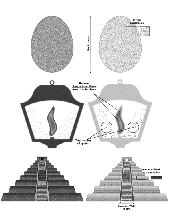
Three hyperproducts were created and displayed using Matlab and Psychtoolbox (BrainardVision, 1997,Pelli, 1997,Kleiner et al., 2007): Golden Eggs, Victorian Lanterns and Mayan Pyramids.2 They were designed to be pleasant to view and intuitively valuable, although participants would have been highly unlikely previously to have valued or traded anything like them. Each hyperproduct could vary on two attributes (see Figure 1). For the Golden Egg, the overall size and the fineness of the surface texture (highest spatial frequency component) varied. For the Victorian Lantern, the ratio of inner to outer flame and the number of sparks emitted from the base varied. For the Mayan Pyramid, the width of the staircase and the moldiness of the bricks varied. In fact, attributes corresponded to standard visual stimuli used in previous discrimination tasks: size, texture, ratio, numerosity, interval, and colour saturation.
It is important to distinguish the objectively defined value of the product, which we simply term the “value”, from the number on the price tag, which we term the “price”. The difference between the two defined the surplus. Value depended on a single attribute magnitude, based on what we term the “value function”:
| Vhct = βh0 + βh1 xtα(c), xt∈[0,1], α(c) ∈ | ⎧ ⎨ ⎩ | 1, |
| , |
| ⎫ ⎬ ⎭ | (1) |
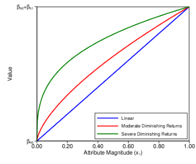
where Vhct is the value of hyperproduct h on trial t for condition c in Euro, βh0 is the minimum value in the range, βh1 scales attribute magnitudes onto the price range, xt is the normalised magnitude of the relevant attribute on trial t, and α(c) defines the degree of diminishing returns. The value of α(c) was therefore the primary manipulation. It was defined as α(c) = (4−c)/3 and took one of three values: α(1) = 1 (linear), α(2) = 2/3 (moderately diminishing returns), and α(3) = 1/3 (severely diminishing returns). Figure 2 depicts these three cases.
The price range varied by product: €180–420 for the Golden Egg; €7–35 for the Lantern; and €23,000–172,000 for the pyramid. The three main conditions, c ∈ {1,2,3}, corresponded to levels of α(c). These were pseudo-randomized across participants and attributes, with the proviso that the two attributes of each hyperproduct had different c. When the range, r ∈ {high,low}, of attribute magnitudes was “high”, close to the maximum feasible range was used. When it was “low”, this was halved. Overall, therefore, there were three main conditions, c, counterbalanced over three hyper-products, h, and two range conditions, r. The 18 possible combinations were pseudo-randomized across the 36 subjects.
While multiple factors were manipulated and counterbalanced, the task was essentially simple. For Experiment 1a, participants saw a hyperproduct and a price tag. Their job was to decide whether the product was worth more or less than its price. Participants had little or no difficulty understanding the task. Responses were collected via a response box.
Participants received intensive one-to-one instruction from the experimenter and could ask questions at any time. They completed six experimental runs. Before each run they were introduced to the single relevant attribute and its relationship to the price. The experimenter first showed the average magnitude and the amount it was worth. This was followed by an evenly spaced ascending sequence of examples across the range, designed to demonstrate how value increased with the attribute magnitude. The aim was to demonstrate the nonlinearity as clearly as possible, as we were interested in the application of the function, not its acquisition (HammondSummers, 1972). Systematic rising sequences quicken learning (Busemeyer et al., 1997).
Participants then undertook eight practice trials. Pilot work suggested that using sequential examples followed by eight practice trials was sufficient for consistent estimation across a test run. Nevertheless, an advantage of the S-ID task is that performance over trials can be tracked and adjustments to measures made if performance improves across the run, although based on the pilot, this was not anticipated. Following the example sequence and practice trials, participants undertook 72 trials at their own speed, with breaks between runs and a longer refreshment break after three runs. Sessions typically lasted just under an hour.
The surplus, Δt, on each trial was selected using an adaptive method of constant stimuli (MCS) — a standard procedure for improving the accuracy of measures of discrimination. Figure 3 depicts how the procedure worked for a typical run. The trials consisted of nine blocks of eight, which each contained symmetric positive and negative surpluses spanning degrees of difficulty, presented in a random order. Within a block, Δt corresponded to four positive and four negative surpluses, Δt ∈ {7δ, 5δ, 3δ, δ, -δ, -3δ, -5δ, -7δ}, where δ was a proportion of the mean price. If the participant responded correctly on seven or eight of the trials, δ was reduced for the next block; if six were correct, δ remained unchanged; if less than six, δ was increased.3 On each trial, the price and value were selected by drawing a price, Pht, from a uniform distribution, adding the surplus to obtain the value, i.e. Vht=Pht+Δt, then calculating the relevant attribute magnitude, xt, according to eq:oneval. Hence, at all prices the probability of a positive surplus was always 0.5. The nonrelevant attribute magnitude was selected randomly.
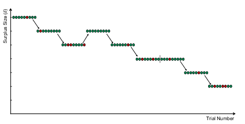
Figure 3: Example implementation of the adaptive method of constant stimuli. The experimental run consisted of 9 blocks of 8 trials as shown. Green dots denote a correct response; red dots, an incorrect one. When the participant achieved 7 or 8 correct responses within a block, the surplus sizes were reduced for the subsequent block. Less than 6 correct responses resulted in an increase in the subsequent block; 6 correct responses meant that the surplus was left unchanged. By ensuring sufficient correct and incorrect responses, the adaptive procedure improves estimation of the participant’s JND.
The hyperproduct and price were displayed until the participant responded. Responses triggered feedback. A green tick or a red cross indicated whether the response was correct, together with an auditory beep for an incorrect answer. The true value, Vht, was presented and remained onscreen until the participant pressed a “Next” button.
Experiment 1b was identical to 1a except that two hyperproducts appeared alongside each other. One had an attribute magnitude calculated as for Vht, the other as for Pht. For example, participants were simply asked to decide which of the two eggs was the largest (a size discrimination), or which of the two lanterns produced fewer sparks (a numerosity discrimination), and so on. No numbers were shown onscreen in experiment 1b. Feedback in this task consisted merely of a tick or cross (and beep).
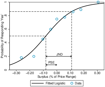
In the S-ID task, bias and precision are quantified via standard measures used in detection theory: the point of subjective equality (PSE) and the just noticeable difference (JND). Both correspond to parameters of the best fitting logistic psychometric function (Figure 4). The dependent variable is whether the participant responded that the surplus was positive. The surplus magnitude is a continuous explanatory variable. When surplus is very high, participants respond that it is positive; when it is very low they respond that it is negative, but intervening levels produce probabilistic responses. The PSE equates to the surplus at which participants are equally likely to decide that it is positive or negative. Hence, a negative PSE indicates overestimation of surplus; a positive PSE indicates underestimation. The JND is determined by the slope of the psychometric function. It is the difference in surplus required for the probability that the participant detected a positive (or negative, since the psychometric function is symmetric) surplus to rise from 0.5 to 0.86, equivalent to one standard deviation of the logistic distribution. Thus, for an unbiased subject, the JND measures the amount of surplus needed for 86% correct identification.
Figure 4 illustrates a psychometric function for a single run in Experiment 1a. The surplus magnitude is expressed as a proportion of the overall price range (results to follow provide the rationale for this). More formally, we model the probability of a positive response by the logistic formula,
| Pr(‶Yes") = exp(θ0 + θ1 Surplus)1+exp(θ0 + θ1 Surplus). (2) |
For the example data in Figure 4, the coefficients are θ0=0.77 and θ1=9.50. From the standard properties of the logistic function it is straightforward to derive the PSE, −θ0/θ1=−8.1%, and JND, π/(θ1√3)=19.1%. These numbers imply that the example participant overestimated surplus by 8.1% of the price range and required a 19.1% higher or lower surplus to increase the probability of a correct response from 50% to 86%.
Our main hypotheses straightforwardly translate into changes in the slope and location of the psychometric function. If a participant is less precise when the value function is nonlinear, the slope of the psychometric function that relates surplus to the likelihood of assessing it to be positive becomes shallower, increasing the JND. If nonlinear value functions induce bias, the psychometric function shifts location. Specifically, linearization of a concave function implies a shift to the right for products valued near the middle of the range, as value would be underestimated relative to products at either end (see Figure 2).
For ease of interpretation, we present mostly mean PSEs and JNDs. For significance testing, we employ a generalized linear mixed model (GLMM), which increases statistical power relative to a comparison of individual means (Moscatelli et al., 2012), although in practice results are closely similar. The model simultaneously fits a logistic function to the data for all participants and trials. Individual differences are accounted for via random effects that assume normally distributed variation in bias and precision across individuals, with a correlation between the two. Surplus, condition, and price are specified as covariates. A significant change in PSE is indicated by a significant coefficient on a condition (or price), which implies that the location of the logistic curve shifts for the given condition (or price). A change in JND is indicated by a significant interaction between the surplus and a condition (or price). A positive interaction implies higher precision — the slope of the psychometric function steepens for the given condition (or price). A negative interaction indicates loss of precision — the slope is more shallow. A more detailed description and full model output is provided in the Appendix. In the following subsection we report relevant coefficients, standard errors, and p-values.
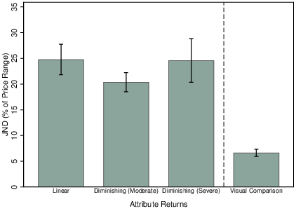
Figure 5 reports the JNDs by linearity condition. The choice of units for the vertical axis is important. Surplus can be expressed in various ways: absolute monetary amount, proportion of the price, proportion of the price range, etc. In fact, across the three different hyperproducts (and associated price ranges) and six attributes, Experiment 1a produced striking consistency when surplus was expressed as a proportion of the price range. To identify surplus reliably, participants required it to exceed 20-25% of the price range. As Figure 5 shows, this was three to four times greater than the mean JND in Experiment 1b, in which participants instead discriminated between two visual attribute magnitudes, with no prices.4 This high level of precision in Experiment 1b confirms the effectiveness of the stimuli: attribute magnitudes were easily perceived and participants could discriminate between them with expected levels of precision based on previous measures of visual discrimination for similar perceptual stimuli (Morgan, 1991). However, this did not translate into similarly precise surplus discrimination when trying to compare the same attributes against prices.
The hypothesis that nonlinear value functions reduce precision was not confirmed. Column (2) of Table 3 (Appendix) presents the full GLMM output underlying our significance tests. We find no evidence that precision was impaired by nonlinearity, whether severe (β=−0.05 (0.58), p > 0.25) or moderate (β=1.53 (0.55), p > 0.99). As suggested by Figure 5 and confirmed by the latter positive coefficient and high p-value, when the attribute had moderately diminishing returns there was in fact a slight advantage. Further investigation (Table 3, column (5)) shows that this effect, which was the opposite of that hypothesised, occurred only when the attribute range was low and was not statistically significant when the range was high (β=0.69 (0.62), p > 0.25). Overall, halving the attribute range produced a significant reduction in precision: β=−1.66 (0.48), p < 0.01 (Table 3, column (3)). The implication is that reducing the perceptual discriminability of attributes did affect precision when trying to determine surplus. However, in addition to the abovementioned inconsistency across conditions, this effect was relatively small: mean JND climbed from 20.7% (high) to 25.8% (low).
The more striking result is that precision was in no way diminished by the presence of a strong nonlinearity. The JND for the high range in all three conditions was close to that previously recorded in an experiment that used only linear attribute returns (Lunn et al., 2020), implying performance in the nonlinear conditions that was better than expected.
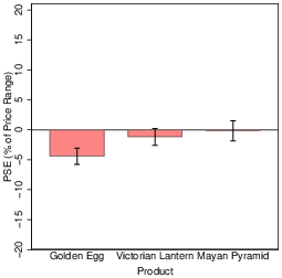
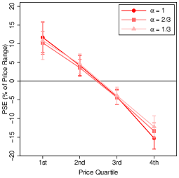
Our second main hypothesis was that nonlinearity would induce bias, specifically linearization. For a concave function, this implies underestimation near the middle of the range. In Experiment 1a, overall, there was a slight overestimation of 1.7% of the price range — see column (1) of Table 3 for the underlying parameter bias estimates. This small bias was driven by the Golden Egg hyperproduct, as shown in the left panel of Figure 6 and in column (4) of Table 3. However, variation in bias across the price range was much larger and followed a different pattern from the one implied by linearization. Participants underestimated surplus substantially near the bottom of the range and overestimated it substantially toward the top (Figure 6, right). Splitting the range into quartiles reveals that for half of all trials (1st and 4th quartiles), surplus was misjudged by more than 10% of the price range. Most important for present purposes, this bias was consistent across the main conditions and, thus, unaffected by strong nonlinearities in the value function. Furthermore, this bias was consistent across all attributes, price ranges, and value functions. Contrary to our hypothesis, therefore, participants had no tendency to linearize the function. A similar bias across the range for a single product with linear returns was reported by (Lunn et al., 2020). Here, unexpectedly, it generalized to nonlinear functions.
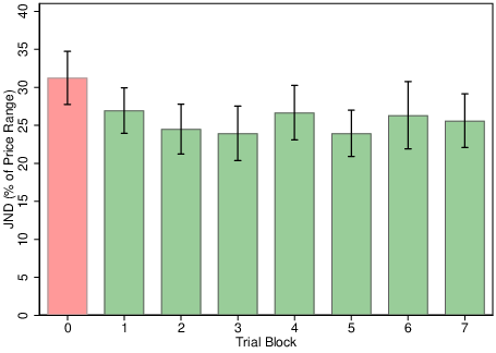
Given these surprising results, we examined variation across participants (Figure 7). One standard deviation in JND equated to approximately 6 percentage points. No participant in any condition generated a JND below 12% of the price range. Thus, the JNDs of even the best performers were double the mean JND recorded in Experiment 1b. There was no evidence of bimodality in the data, which might have suggested that some participants did not properly understand the task. The box-plot hints that perhaps a small minority found the strong nonlinearity more difficult. But not only was any overall difference short of statistical significance, the point estimate for median precision was better than in the linear condition. There was modest variation in bias across individuals too, but the most striking result was the consistency of the pattern across the price range. All participants overestimated surplus at the top and almost all underestimated it at the bottom, with a clear shift in the entire distribution as the price increased. No participant linearized even the strongly nonlinear value function.
As described above, the experiment was not designed to investigate the learning process. Rather, one-to-one instruction, example sequences, and practice trials were developed to make learning the value functions as easy as possible. We nevertheless checked for variation in performance across experimental runs. Figure 8 shows the consistency of the JND following initial practice trials. We generated this graph by adding interaction terms for each trial block added to the baseline model in column (1) of Table 3. Participants were significantly less precise in the practice trials relative to the trials that followed (β=−1.63, z=−5.18, p< 0.001), but there was no improvement thereafter, in keeping with the experimental design and our pilot work. Similarly, there was no change in the pattern of bias across trials, despite strong feedback.
Table 1: Value Function Estimates.
Value function: β0 β1 α λ Number of Individuals Number of Observations Individual-cluster-robust bootstrapped 95% confidence intervals in brackets.
The overall null result means that it is important to be sure that participants internalized the different value functions across the main conditions. In theory, participant confusion or high imprecision due to task complexity could have masked true differences across condition, although participants were given one-to-one instruction and reported no difficulty understanding the task in the debriefing sessions. Empirically, we can test whether participants’ responses indicate that they had learned different functions.
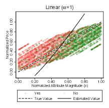
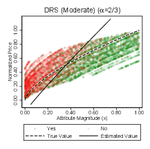
To test whether participants learned and applied different value functions, we can compare their responses for a given attribute magnitude and price across conditions. Figure 9 plots the raw response data, with attribute magnitude, x, on the horizontal axis and price, P, on the vertical axis. Red dots indicate “no” responses (no surplus) and green dots indicate “yes” responses (surplus). Dashed lines correspond to the true value function. There are clear differences in the curvature of participants’ responses across treatments, indicating that they internalized and applied three separate functions of varying linearity. The solid lines represent our best-fitting estimate of the average internal value function implied by participants’ responses. To generate these functions, for individual i on trial t we estimated,
| Vit = β0 + β1 xitα+ λ ε (3) |
where ε is a logit error with scale parameter λ, and xit is the normalized attribute. β0 and β1 determine the location and overall slope of the applied value function, while α determines the curvature. Given this functional form, we estimated (β0,β1,α,λ) separately for each experimental condition using maximum likelihood estimation.
Figure 9: Dots represent observations at a given attribute magnitude and price. Red dots denote a “No” response, green dots, a “Yes”. Dashed lines depict true value functions. Observations below dashed lines had a positive surplus and observations above had a negative surplus. Solid lines depict best-fitting value functions based on the parameters estimates in Table 1.
Table 1 presents estimated parameters. Across the three conditions the intercept, slope, and error parameters are similar, with β1 exceeding one, consistent with the strong bias across the price range. By contrast, the curvature, α, differs markedly. A likelihood ratio test provides a strong rejection of the null hypothesis that α is constant across conditions (p<0.001). Of course, these estimated functions based on the response data are far from veridical, and the estimation assumes a functional form that matches the true value functions. We make no claim that the relevant cognitive mechanism operates by applying such a function. Nevertheless, the results demonstrate that participants absorbed and attempted to apply value functions of substantially different curvature.
A key point is that while the strong bias in responses shows that the functions applied by participants did not match the true functions, the consistency of this bias across conditions in Figure 7 (right) indicates that their internalized value functions differed strongly in linearity. If confusion or general imprecision had driven our results, we would not see this consistency, which is matched by the consistency of the difference between the solid and dashed lines across the conditions in Figure 9. Hence, participants applied different degrees of curvature to assess surplus, but this was not a limiting factor in the precision and bias of responses. Overall, the data indicate that participants learned and applied different functional forms across our experimental treatments, with the null finding stemming from a legitimate lack of performance differences across the shape of the value functions.
Our primary hypotheses did not hold. For single-attribute products, a strong nonlinearity in the functional relationship between the attribute magnitude and the product’s value had no significant impact on the precision with which surplus could be assessed. Moreover, we observed a substantial bias across the price range that was not consistent with a tendency to linearize nonlinear relationships. Participants demonstrably adopted and attempted to apply different functions with different degrees of curvature. The severity of monotonic nonlinearity was large relative to estimates of early perceptual nonlinearities (Stevens, 1975). Yet participants accomplished nonlinear internal mappings of scales with the same accuracy as linear ones. This rapid learning of openly demonstrated linear mappings matches previous work on acquisition versus application of functions (Deane et al., 1972,HammondSummers, 1972), but the equivalent accuracy for nonlinear functions does not.
This is an important null result. A systematic impact on precision or bias when trying to apply nonlinear preferences would need to be reflected in models of consumer decision making. Previous empirical findings concerning judgment of nonlinear functions implied that such an impact was likely in a simple setting where individuals compared a single attribute against a price. Having set out to confirm this, we instead found that accuracy was unaffected by a strong nonlinearities in monotonic, concave functions, across a variety of attributes and numeric price ranges. The experimental design involved over 15,500 observations, which is high compared to the typical function learning studies that motivated our investigation (KohMeyer, 1991,DeLosh et al., 1997,KarelaiaHogarth, 2008). Statistical power was sufficient to detect a 5 percentage point improvement in JND between the high and low range conditions with p=0.002 and between practice and test trials at p<0.001. Similarly reliable differences by linearity would also have been detected, but simply did not arise. In fact, point estimates of median JNDs were marginally lower in the nonlinear conditions, with a lower mean also in the α=2/3 condition.
In the context of consumer decisions, the JND in Experiment 1a of 20–25% of the range for 86% reliability may seem intuitively high. Yet it is in keeping with other work. (Lunn et al., 2020) (Experiment 1) recorded a median JND of 20% using an attribute range similar to the “high” condition used here. That study employed only linear relationships and compared the performance of a sample of consumers against a sample of quantitative professional researchers competing in a tournament (Experiment 2). Performance in this present study was closely similar. This undercuts the possibility that an underlying effect of nonlinearity was somehow masked, perhaps by participants being asked to apply value functions of different linearity to different attributes within the same experimental session. The overall level of precision in any case tallies with some related tasks. JNDs were broadly constant across manipulations when expressed as a proportion of the range, with most participants requiring a difference of between one-quarter to one-ninth of the range to identify a surplus reliably (in the high range condition). This limit on precision echoes the constraints in absolute identification tasks first emphasized by (Miller, 1956) and reviewed by (Cowan, 2010). Together with the striking consistency in the pattern of bias across value functions, it suggests a process that adjusts perceptual stimuli to internal scale values before mapping them to another scale (Anderson, 1974), in this case a representation of numeric prices.
This ability to assess surplus is an important skill for consumers. The implication of the present results is that the cognitive mechanism involved is flexible but coarse. New relationships can be processed rapidly, including transforming nonlinear scale values, but Experiment 1a shows that the mechanism is subject to substantial imprecision and bias. Across multiple products, attributes, price ranges, and value functions, when mapping a single attribute to a price, precision in Experiment 1a was greatly diminished relative to Experiment 1b, when discriminating between relative attribute magnitudes using the same stimuli. Meanwhile, the mapping was oversensitive to attribute magnitudes relative to prices, such that the top and bottom quartiles of the range were strongly overestimated and underestimated, respectively.
Given that our initial hypotheses turned out not to hold, Study 2 was more exploratory in its aims. Attribute-price relationships are usually more elaborate than unidimensional monotonic functions. Our rationale was to introduce multiple realistic properties of products and to test whether they generated a change in relative performance between linear and nonlinear functional forms. This was achieved in four ways.
First, products typically have multiple attributes. Having to consider multiple attributes is likely to increase cognitive load. As argued by (BrehmerSlovic, 1980), if adjusting internal scale values to match a nonlinear function does likewise, nonlinearities might not affect performance in a unidimensional context but may do so in a multidimensional one. In our case, nonlinear returns embedded in multiattribute products may be more disruptive than when embedded in single-attribute products.
Second, when products have multiple attributes, some are generally more important to consumers than others. Sometimes the magnitude of one attribute can logically negate the importance of the other, such as when a full guarantee removes worries about reliability. More generally, the requirement to “weight” attributes could interact with the need to process a nonlinearity. The initial adjustment of scale values could alter the decision weight given to the adjusted attribute. Weight might increase because of additional attention given to the specific attribute (Armel et al., 2008,Krajbich et al., 2010), or decrease because processing of the attribute is less fluent (ShahOppenheimer, 2007).
Third, while diminishing returns are perhaps the most common nonlinearities in preferences, other nonlinear functional forms also arise. Returns can be increasing. A city worker who loves the countryside may get increasing returns from living further from the city center. Returns can also be nonmonotonic. Some attributes can be too small or too large. Consumers may seek a “happy medium”, for instance, when considering the alcohol content of drinks, risk profiles of investments, or sizes of car engine. Cyclical attributes with multiple peaks are also possible: portions may be too big for one, yet too small for two; furniture may be less valuable as it ages, yet more valuable as it becomes antique; puzzles may be too hard for a child, yet too easy for an adult. Attributes can “fall between stools”. The introduction of nonmonotonic returns in a multiattribute product leads to an intriguing possibility. (Lockhead, 1970) and (MonahanLockhead, 1977) investigated absolute identification of multidimensional perceptual stimuli when one attribute was mapped to an ascending set of stimuli via a nonmonotonic, cyclical function. Participants identified stimuli more accurately than when the same dimensions were monotonically related. The implication was that participants integrated stimuli into a multidimensional representation, with accuracy predicted by the distance between stimuli in multiattribute space. If surpluses conferred by multiattribute products are processed similarly, accuracy may hold up, or even improve, for nonmonotonic preference functions.
Fourth, many attributes are communicated to consumers numerically. By instead employing only visual attributes in Study 1, we may have underestimated potential performance. The reason for not using single numeric attributes was that it would have allowed participants to memorize one-to-one pairs or deploy arithmetic rules, undermining the testing of our main hypotheses. With a multiattribute product, however, the same problem does not apply. Accuracy when products consist of one numeric attribute and one visual attribute can be compared with accuracy when products consist of two visual attributes. Neither task permits reliable numeric mappings or arithmetic.
One advantage of the S-ID task is that it generates rich data that allow multiple experimental manipulations to be undertaken simultaneously. Given the common occurrence of multiattribute products, differential attribute weighting, nonmonotonic returns and numeric attributes, Study 2 explored the impact of each.
Methods were as in Experiment 1a, except for the following modifications.
Twenty-four consumers were recruited through a market research company (14 female; mean age = 34.7, SD = 13.0; 13 employed).
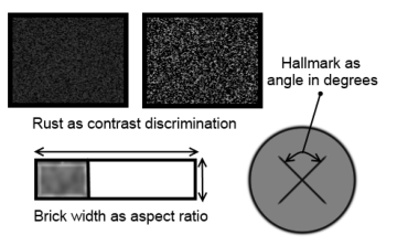
Six additional attributes were employed. Three, one for each hyperproduct, were visual (see Figure 10). On the Golden Egg, we varied a quality hallmark, with magnitude defined as the angle subtended by two intersecting lines. On the Victorian Lantern, we varied “rustiness”, defined as the contrast between an orange-brown versus a black colored texture. On the Mayan Pyramid, we varied the flatness of the bricks, defined as the rectangular aspect ratio. These stimuli were selected on the basis of the human ability to discriminate angles, contrasts, and shapes with high precision. The other three attributes were numeric and appeared next to each hyperproduct. For the Golden Egg, we displayed purity in karats; for the Victorian Lantern, fuel efficiency was given on a 25-point scale; for the Mayan Pyramid, we gave the age in years.
In the two-attribute case, equation eq:oneval becomes
| Vhv=βh0+βh1 fv (x1,α1, x2,α2), fv(·) ∈[0,1], α1+α2=1 (4) |
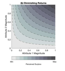
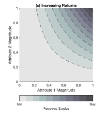
where v denotes one of six value functions and the β terms map the overall product magnitude, fv(·), onto the price range for hyperproduct, h. Table 2 shows the six functional forms. Function (1) was linear, with perfectly separable attributes. Function (2) had constant returns to scale overall, but diminishing returns (DRS) per attribute. This function is a Cobb-Douglas preference function commonly deployed in microeconomic models. Function (3) exhibited increasing returns (IRS). Function (4) was another standard preference function (Leontief) with a logical relationship between attributes, which are perfect complements. The product is only as good as its weakest attribute. Function (5) combined an attribute with linear returns and a nonlinear, cyclical attribute. Finally, function (6) had nonmonotonic returns to both attributes, such that the center of the attribute space defined a perfect product. We called this the“goldilocks” value function, because the product price corresponded to distance in attribute space from “just right”, (x1,x2)=(1/2, 1/2), attribute levels.
Table 2: Value function specifications in Study 2
(1) Perfect Substitutes (linear) α1 x1 + α2 x2 (2) Cobb–Douglas (constant returns to scale) x1α1 x2α2 (3) Cobb–Douglas (increasing returns to scale) x13α1 x23α2 (4) Leontief max(α1,α2) min(x1/α1,x2/α2 ) (5) Cyclical α1 x1+α2sin(2π x2)+1/2 (6) Goldilocks 1−4/1/α12+1/α22 [ (x1−1/2/α1)2 +(x2−1/2/α2)2 ]
Participants completed one run per value function. Each began with a learning phase that explained the value function and presented examples of hyperproducts and prices, designed to facilitate rapid learning, as in Experiment 1a. Participants received intensive one-to-one instruction. The value function was explained and demonstrated via a sequence of examples that systematically varied each attribute in turn across its range. Participants then undertook eight practice trials and 56 test trials (t).
Given two attributes, any value, Vhtz, could be generated by infinite combinations of x1t and x2t. We selected these at random. To manipulate attribute weighting, while α1 and α2 always summed to one, they were balanced for half the runs (i.e. 1/2,1/2; b=1) and unbalanced for the other half (2/3,1/3 or 1/3,2/3; b=2), such that one attribute had twice the weight of the other. Value functions, products, combinations of attribute pairs, and attribute balance were pseudo-randomized across participants and runs.
As described above, Study 2 explored four additional aspects of the value function. We describe the impact of each in turn.
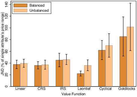
JNDs by condition are shown in Figure 11. The first three categories offer a straightforward comparison between the linear and nonlinear monotonic value functions. Overall, the introduction of a second attribute decreased precision relative to Experiment 1a. Surplus needed to be the equivalent of 36–46% of an attribute range for reliable detection. This level of imprecision did not differ significantly between the linear and the CRS function. Thus, even when participants were juggling multiple attributes, precision was unaffected by diminishing returns to attributes. There was a small but statistically significant decrease in precision for the IRS value function consistent with Figure 11 (β=−0.72, z=−2.53, p<0.05; see column (1) of Table 4 in the appendix).
Figure 11 also reveals that any impact of differential attribute weighting was minor. While point estimates for JNDs were marginally higher, the overall difference was not statistically significant. The one exception was for the Leontief value function, where unbalancing the attribute weighting reduced precision (β=−2.95, z=−3.35, p< 0.001). With balanced attributes, participants had little problem determining which one was weaker and so the JND approached a level similar to that recorded for single attributes in Experiment 1a. With unbalanced attributes, participants found it more difficult to determine which attribute was the weaker of the two, reducing precision. Aside from this difficulty, any additional cognitive load induced by differential balancing of attributes had little impact on the processing of nonlinear value functions.
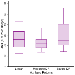
Precision was greatly reduced for nonmonotonic nonlinear value functions. For the combination of linear and cyclical attributes, the JND rose to 60-70% of an attribute range, while for the Goldilocks function it was as high as 80-100%. These increases are large and statistically significant (cyclical, β=−1.91, z=−4.78, p< 0.001; Goldilocks, β=−2.70, z=−9.05, p< 0.001).
There was a statistically significant improvement in precision when attributes were numeric (β=0.55, z=2.47, p< 0.05; see column 2, of Table 4). However, the size of this effect was small in comparison to the difference between monotonic and nonmonotonic nonlinearities, equivalent to a decrease in JND for a monotonic value function from 42% of an attribute range to 37%.
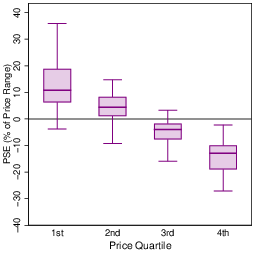
Figure 12 plots bias across the price range by value function. Despite the great differences in the shape of value functions and much lower precision for nonmonotonic functions, the downward-sloping bias across the price range occurred in all conditions. The bias was again substantial, equating to differences in surplus between the lowest and highest quartile of approximately one JND. The only difference specific to a value function was a general tendency to overestimate surplus for the Goldilocks function, which nevertheless retained the downward-sloping relationship.
We find that there was a moderate improvement in precision between the practice trials and the main experimental trials (β = 0.42, z = −1.65, p < 0.1). However, we find no evidence of further learning within the main experimental trials. Separating each run into four blocks of trials, we find that compared to the first block of trials, surplus detection was no more accurate in the second (β = 0.05, z = 0.24, p > 0.25), third (β = 0.17, z = 0.21, p > 0.25), or fourth (β = −0.18, z = 0.20, p > 0.25) blocks.
While there was a clear drop in precision associated with the nonmonotonic value functions, Study 2 replicated the finding of Experiment 1a that surplus for a monotonic nonlinear function with diminishing returns (CRS) can be assessed as accurately as that for a linear function. As described above, the less common value function with increasing returns (IRS) may have marginally reduced precision. Again, given a null result, it is important to confirm that participants had absorbed and attempted to apply different functions, in this case also incorporating the magnitudes of both attributes. As in Section 3.2.6 for Experiment 1a, we estimated the best-fitting value functions to responses. In the two-attribute case,
| Vit = β0 + β1 f(x1it,x2it,α1,α2) + λ ε (5) |
where ε is a logit error with scale parameter λ, x1it and x2it are the normalized attribute magnitudes, and f is defined as in Table 2. From the fitted parameters we then generated indifference curves for the linear, CRS, and IRS value functions. These are displayed in Figure 13. The indifference curves are highly nonlinear in the CRS and IRS conditions. As in Experiment 1a, participants had absorbed and applied the nonlinearity when faced with both of the monotonic nonlinear value functions.
Study 2 confirms the central findings of Study 1 and generates several new results. The requirement to consider two attributes (in addition to price) resulted in a loss of precision when identifying surplus, producing JNDs higher than in Experiment 1a. Nevertheless, performance when attributes had diminishing returns was almost identical to that when returns were linear, with no tendency to linearize the relationship. Participants had again clearly internalized and applied different value functions, producing responses consistent with strongly nonlinear indifference curves. Notwithstanding the marginal effect when returns were increasing, the additional cognitive load associated with integrating the additional attribute did not alter the main finding of Study 1. The ability to identify a surplus seems to be substantively unaffected by the need to process monotonic nonlinearities. Also consistent with Study 1, perceptual error played only a small role in performance, given the marginal improvement in JND induced by numeric attributes. The mapping of internal scales, rather than their origin, primarily determined performance.
Nevertheless, in Study 2 we did observe clear variation in precision, which was impaired when value functions had nonmonotonic returns. The need to compare attribute magnitudes against “just right” points retained in memory increased JNDs substantially. This contrasts with the results from absolute identification tasks using multidimensional perceptual stimuli (Lockhead, 1970,MonahanLockhead, 1977). While it may be easier to identify a stimulus as one of a learned set based on distance in multidimensional space, the same logic does not apply to mapping multidimensional stimuli to another scale (in this case price). The strong bias across the price range was also consistent with Study 1. Its prevalence across such a wide variety of value functions is striking and we consider potential causes in the General Discussion section. Study 2 allows us to rule out one possibility, however. When the value function is monotonic, successive presentations of visual stimuli might generate contrast effects that exaggerate differences, causing an upward adjustment of high-value products and downward adjustment of low-value products. However, the same bias emerged for nonmonotonic value functions, to which this logic does not apply. Furthermore, if this was the cause, the bias should have weakened when one attribute was numeric, yet it did not.
Spotting when a product is good value is a fundamental skill of economic decision making. Based on studies of judgment going back many decades, we hypothesized that, where returns to attributes are nonlinear, people’s ability to identify good value would diminish appreciably. This was our primary hypothesis, but it was not supported. Experimental participants were able to cope with monotonic nonlinear mappings of attributes to prices without additional bias or imprecision, relative to linear mappings, with both single-attribute and multiattribute products. Moreover, the patterns of responses clearly indicated that participants absorbed and applied value functions that, while not veridical, differed strongly in linearity. We think it highly unlikely that our results constitute a Type 1 error. The null results arose in two studies that employed large samples relative to previous work and which detected relatively small differences in precision due to other factors (range, practice versus test trials, numeric versus visual attributes). In all three direct comparisons of linear value functions against functions exhibiting diminishing returns, point estimates of median precision were marginally better in the nonlinear case, while point estimates of mean precision were better in two out of three. We conclude that difficulty processing nonlinear scales in one type of task does not necessarily transfer to another type of task, in this case one designed to mimic consumer decisions.
Our findings imply that when a monotonic nonlinear relationship is described and demonstrated to consumers, they are able to undertake the necessary mapping of internal scales to process it. One should not infer, however, that monotonic nonlinearities cause no problems, because consumers need to realize to begin with that the relationship is nonlinear. We went to some length to show our participants the relevant nonlinearities, through examples and feedback. In real-world settings, consumers are not so fortunate. They may not grasp the shape of the relationship between say, interest rates and the financial cost of a loan, or miles-per-gallon and the cost of motoring. Hence some consumers may linearize such relationships, even if our findings suggest that they could learn to process them if given clear examples and a bit of practice.
Nevertheless, the null finding for monotonic nonlinearities is of some comfort from the perspective of models of consumer choice, which typically assume that the shape of preferences does not affect the distribution of error when applying preferences to a decision. Of less comfort, and consistent with the hypothesis, when value depended on nonmonotonic nonlinear functions, there was substantial loss of precision. This finding favors approaches to internal scaling that, unlike standard microeconomic models, do not assume internal representation of absolute stimulus values. For instance, in the relative judgment model (RJM) (Laming, 1997,Stewart et al., 2005), a current stimulus is judged by comparison to representations of only a subset of recently encountered or available stimuli. If attributes are primarily scaled using a relative coding like this, one would anticipate that turning points in preferences would lead to inaccuracy, as they require comparison with an absolute stimulus level. An internal representation based on relative distance from a sparse subset of stimuli would become unreliable.
More generally, despite being able to process monotonic nonlinearities, participants’ absolute levels of performance in the S-ID task imply severe limits to the granularity of attribute coding, constraining consumers’ ability to identify surpluses. Whether linear or nonlinear, the mapping of attributes to prices is coarse and subject to systematic bias. Across multiple products, attributes, and price ranges, when surplus was determined by a monotonic function applied to a large discriminable range, a surplus of 20% of that range was required for most participants to detect it reliably, with a standard deviation across individuals of around 6 percentage points. The implication is that, absent explicit arithmetic or memorized one-to-one mappings, consumers can reliably discern about four to seven levels of value across a range, perhaps up to nine for the top performers. These numbers correspond closely to the seminal work of (Miller, 1956) and more recently (Cowan, 2010). Similar constraints seem to apply to both the mapping of continuous product attributes to prices and the mapping of perceptual stimuli to categories in absolute identification studies.
Interestingly, however, while participants displayed systematic biases in the S-ID task, as they do in absolute identification and magnitude estimation tasks, the pattern of bias was essentially reversed. Instead of a central tendency bias (Laming, 1997,MatthewsStewart, 2009), surpluses at the bottom of the range were underestimated and those at the top overestimated. The difference is presumably related to the requirement in the S-ID task to discriminate stimulus magnitude(s) against a numeric price — the defining element of consumer choice. All participants displayed the bias and its magnitude was substantial. The same bias was recorded for linear value functions by (Lunn et al., 2020). In the present paper, we hypothesized bias due to linearization, but found no evidence for it. Instead, this systematic bias across the price range was consistent across all value functions: linear, nonlinear, monotonic, or nonmonotonic. We are otherwise unaware of previous relevant reports in the judgment and decision-making literature or broader consumer research. Yet the scale and scope of the effect are striking and imply that bias arises after internal scale values are adjusted to reflect nonlinearities in value.
The bias could indicate a fundamental normalization process when scales must be mapped and discriminated. We note that some studies of perceptual decision making have sought to explain biases across a stimulus range that similarly persist despite practice and feedback (De GardelleSummerfield, 2011,Michael et al., 2015). Building on (Barlow, 1961), (SummerfieldTsetsos, 2015) argue that precision and bias trade off within a neural system that seeks to optimize decisions given constrained capacity. The logic is that the limited range of neural signals requires normalisation to specific contexts, which increases discriminability near the middle of a range at the expense of compressing, and thus biasing, signals towards the ends. Our findings suggest that consumer choice, which requires mapping attributes to prices to discriminate surplus, may involve a similar mechanism. Further research is needed to substantiate the scope of this bias, whether an adaptive normalization process explains it, and the contextual factors involved. For instance, the effect might be confined to contexts in which decisions are sequential, or indeed might not.
In line with (Deane et al., 1972) and (HammondSummers, 1972), our participants had little problem acquiring nonlinear functions through explanation and demonstration; the difficulty was in applying them. Overall, therefore, the findings are consistent with a mechanism for comparing product attributes against prices that is highly flexible but coarse, and hence prone to imprecision and bias. If so, the measures of accuracy that we report imply that mistakes in consumers’ assessments of surpluses are likely to be frequent and sometimes substantive. While the implications are potentially economically important, therefore, the generalizability of the findings is naturally debatable. Sequential identification of multiple objective monetary surpluses may not involve exactly the same mechanisms as nonsequential or occasional assessment of subjective surpluses. However, the quality of perceptual stimuli and the opportunities for learning and feedback in the present experiments were far superior to most everyday consumer situations. The findings therefore imply important limits in consumers’ capabilities, even when products possess few attributes.
The following is a technical exposition of the GLMM models used to generate the JNDs and PSEs reported in the main text, together with full tables of coefficients. The explanation focuses on Experiment 1a. The technique is essentially identical across the experiments and closely follows Moscatelli2012. We estimate the following model:
| In | ⎡ ⎢ ⎢ ⎣ |
| ⎤ ⎥ ⎥ ⎦ |
| = (φ0 + µi) + (γ0 + υi) sit + φ zit + γ zit * sit (6) |
where sit is the normalized surplus for individual, i, on trial, t. The fixed effects coefficients are denoted by φ0, γ0, φ and γ. The model has normally distributed random effects, µi and υi with correlation corr(µi,υi).5 zit is a vector containing the experimental manipulations of interest and any other variables or interactions of potential interest. zit enters both individually and as an interaction term with surplus, sit. The vector of coefficients φ therefore determines how bias varies across experimental conditions, while γ determines variation in precision.
As an example, consider the GLMM model used to generate Figure 11. In this specification, we estimate equation eq:logitglmm with just dummy variables for the balance condition, each value function, and their interaction terms. Using the properties of the logistic distribution, the average JND and PSE for a given value function, v, and balance condition, b, are given by
| JNDv,b= |
| . |
| (7) |
| PSEv,b=− |
| (8) |
where each φ term is the estimated coefficient for the appropriate condition and each γ is the estimated coefficient for its interaction with the surplus. Thus, γv*b is the coefficient for the interaction between the dummy variable for a given value function, a dummy variable indicating attribute balance, and the surplus. We then use the coefficient estimates from this GLMM specification and equation eq:jnd to generate the bars in Figure 11.
Table 3: GLMM Results from Experiment 1
Surplus Constant Normalized Price Range Moderate Diminishing Returns Severe Diminishing Returns Low Attribute Range Victorian Lantern Mayan Pyramid Low Range × Moderate Diminishing Returns Low Range × Severe Diminishing Returns Surplus-Interaction Terms Normalized Price Range Moderate Diminishing Returns Severe Diminishing Returns Low Attribute Range Victorian Lantern Mayan Pyramid Low Range × Moderate Diminishing Returns Low Range × Severe Diminishing Returns Number of Individuals Observations *** p<0.01, ** p<0.05, * p<0.1. Individual-cluster-robust standard errors in parentheses.
Table 4: GLMM Results from Experiment 2
Surplus Constant Normalized Price Range Constant Returns to Scale Increasing Returns to Scale Leontief Cyclical Goldilocks Unbalanced Attributes Numeric Attribute Surplus-Interaction Terms Normalized Price Range Constant Returns to Scale Increasing Returns to Scale Leontief Cyclical Goldilocks Unbalanced Attributes Numeric attribute Number of Individuals Observations ***p<0.01, **p<0.05, *p<0.1. Individual-cluster-robust standard errors in parentheses.
Copyright: © 2021. The authors license this article under the terms of the Creative Commons Attribution 3.0 License.
This document was translated from LATEX by HEVEA.