Judgment and Decision Making, Vol. 14, No. 4, July 2019, pp. 381-394
Revealed strength of preference: Inference from response timesArkady Konovalov*
Ian Krajbich#
|
Revealed preference is the dominant approach for inferring preferences, but
it is limited in that it relies solely on discrete choice data. When a
person chooses one alternative over another, we cannot infer the strength
of their preference or predict how likely they will be to make the same
choice again. However, the choice process also produces response times
(RTs), which are continuous and easily observable. It has been shown that
RTs often decrease with strength-of-preference. This is a basic property
of sequential sampling models such as the drift diffusion model. What
remains unclear is whether this relationship is sufficiently strong,
relative to the other factors that affect RTs, to allow us to reliably
infer strength-of-preference across individuals. Using several
experiments, we show that even when every subject chooses the same
alternative, we can still rank them based on their RTs and predict their
behavior on other choice problems. We can also use RTs to predict whether
a subject will repeat or reverse their decision when presented with the
same choice problem a second time. Finally, as a proof-of-concept, we
demonstrate that it is also possible to recover individual preference
parameters from RTs alone. These results demonstrate that it is indeed
possible to use RTs to infer preferences.
Keywords: response times, preferences, drift-diffusion model, risky choice,
intertemporal choice, social preferences
1 Introduction
When inferring a person’s preferences, decision scientists often rely on
choice outcomes. This is the standard revealed preference approach
(Samuelson, 1938). While very powerful, relying purely on choice data
does have its limitations. In particular, observing a single choice
between two options merely allows us to order those two options (as less
and more preferred); we cannot infer the strength of the preference. That
is, we do not know the confidence with which the person made the choice or
the likelihood that they would choose the same alternative again.
Choice itself is not the only output of the choice process. We are also
often able to observe other features such as response times (RT), which
are continuous and so may carry more information than discrete choice
outcomes (Loomes, 2005; Spiliopoulos & Ortmann, 2017). The potential
issue with RTs is that they are known to reflect many factors, including
subject-level traits such as decision strategy and motor latency
(Kahneman, 2013; Luce, 1986), as well as features of the choice problems
such as complexity, stake size, and option similarity (or attributes)
(Bergert & Nosofsky, 2007; Bhatia & Mullett, 2018; Diederich, 1997;
Fific, Little & Nosofsky, 2010; Gabaix, Laibson, Moloche & Weinberg,
2006; Hey, 1995; Rubinstein, 2007; Wilcox, 1993).
One useful characteristic of RTs is that they often correlate (negatively)
with strength-of-preference. This effect was observed in early studies in
psychology and economics (Dashiell, 1937; Diederich, 2003; Jamieson &
Petrusic, 1977; Mosteller & Nogee, 1951; Tversky & Shafir, 1992) and has
been recently extensively researched using choice models (Alós-Ferrer,
Granić, Kern & Wagner, 2016; Busemeyer, 1985; Busemeyer & Rapoport,
1988; Busemeyer & Townsend, 1993; Echenique & Saito, 2017; Hutcherson,
Bushong & Rangel, 2015; Krajbich, Armel & Rangel, 2010; Krajbich &
Rangel, 2011; Moffatt, 2005; Rodriguez, Turner & McClure, 2014). In
other words, choices between more equally-liked options tend to take more
time. If this relationship is strong, relative to the other factors that
affect RT, then we should be able to infer strength-of-preference
information from RTs.1
Consider the following example. Suppose we are attempting to determine
which of two people, Anne or Bob, has a higher discount factor for future
rewards (in other words, is less patient). We ask each of them the same
question: “would you rather have $25 today or $40 in two weeks?”
Suppose that both take the $40. With just this information there is no
way to distinguish between them. Now suppose Anne made her choice in 5
seconds, while Bob made his in 10 seconds. Who is more patient? We argue
that the answer is likely Anne. Since Anne chose the delayed option more
quickly than Bob, it is likely that she found it more attractive. In
other words, Anne’s relative preference for the delayed option was likely
stronger than Bob’s; she was farther from indifference (i.e., the point at
which she is equally likely to choose either option).
Of course, if Anne and Bob employ different decision strategies (e.g., Anne
chooses based on heuristics while Bob chooses based on deliberation) or
differ on other relevant characteristics (e.g., Anne is smarter or younger)
then we might be misled about their preferences. It is thus an empirical
question whether our example is actually feasible, or merely speculation.
This is a key question that we tackle in this paper.
The answer to this question has potential practical importance.
Consider an online marketplace. A customer might inspect a series of
products but reject them all, making the choice data uninformative.
However, the customer may linger more on certain items, revealing which
ones were most appealing. The online seller could use that information to
target related products at the customer. Or returning to an interpersonal
example, an overloaded clothes salesman might focus their attention more
on customers who hesitate longer before returning items to the rack.
Taking this idea one step further, we might also want to know whether
choice data are necessary to infer preferences, or whether RTs alone could
suffice. In the example with Anne and Bob, we used both the choice
outcome and the RT to rank the two decision makers on patience. While the
RT told us how easy the decision was for each person, without the choice
outcome we could not know whether Anne faced an easy decision because she
was very patient or very impatient. This might lead one to believe that
it is still necessary to observe choice outcomes in order to infer
preferences. However, in theory, all we need is a second RT.
Suppose that both Anne and Bob take 5 seconds to choose between the $25
today vs. $40 in two weeks, but we do not see their choices. Let us
assume, for the sake of this example, that strength-of-preference is the
only factor that affects RT. At this point we can use Anne and Bob’s RTs
to infer their distance from indifference, but we cannot say whether they
were on the patient side or impatient side. Now we ask a second question:
$25 today vs. $50 in two weeks. Relative to the previous question, we
have made the “patient” option more attractive, i.e., we have made the
decision easier for a patient person (e.g., someone who chose the $40) and
more difficult for an impatient person (e.g., someone who chose the $25).
Suppose Anne makes this decision in 6 seconds while Bob makes this
decision in 4 seconds. We can then conclude that Bob is on the patient
side and Anne is on the impatient side. With just two questions we are
thus able to infer their temporal discounting factors (preferences, more
generally). Of course, this procedure assumes a noiseless relationship
between strength-of-preference and RT. In what follows, we investigate
the usefulness of this procedure using more than two decisions (to
compensate for noise in the decision process) and show that the
preferences inferred from RTs can indeed be reliable.
Our work builds on a growing literature focused on sequential sampling
models (SSM) (such as the drift-diffusion model (DDM)) of economic
decision making. The idea of applying SSMs to economic choice was first
introduced by Jerome Busemeyer and colleagues in the 1980s (Busemeyer,
1985) and further developed into decision field theory in subsequent years
(Diederich, 1997, 2003; Roe, Busemeyer & Townsend, 2001). Recent years
have seen renewed interest in this work due to the ability of these models
to simultaneously account for choices, RTs, eye movements, and brain
activity in many individual preference domains such as risk and
uncertainty (Fiedler & Glöckner, 2012; Hunt et al., 2012; Stewart,
Hermens & Matthews, 2015), intertemporal choice (Amasino, Sullivan,
Kranton & Huettel, 2019; Dai & Busemeyer, 2014; Rodriguez et al.,
2014), social preferences (Hutcherson et al., 2015; Krajbich, Bartling,
Hare & Fehr, 2015; Krajbich, Hare, Bartling, Morishima & Fehr, 2015),
food and consumer choice (De Martino, Fleming, Garret & Dolan, 2013;
Krajbich et al., 2010; Milosavljevic, Malmaud, Huth, Koch & Rangel,
2010; Polanía, Krajbich, Grueschow & Ruff, 2014), and more complex
decision problems (Caplin & Martin, 2016; Konovalov & Krajbich, 2016).
The SSM framework views simple binary decisions as a mental tug-of-war
between the options (Bogacz, Brown, Moehlis, Holmes & Cohen, 2006;
Brunton, Botvinick & Brody, 2013; Fudenberg, Strack & Strzalecki,
2018; Shadlen & Shohamy, 2016; Tajima, Drugowitsch & Pouget, 2016;
Usher & McClelland, 2001; Woodford, 2014). For options that are similar
in strength (subjective value) it takes more time to determine the winner,
and in some cases the weaker side may prevail. In other words, these
models predict that long RTs indicate indifference, and that RTs decrease
as the superior option gets better than the inferior option.
Here, we estimate individual preferences using subjective value (utility)
functions with single parameters and demonstrate the strength of the
relationship between preference and RT, using experimental data from three
prominent choice domains: risk, time, and social preferences. We show
that single-trial RTs can be used to rank subjects according to their
degree of loss aversion, that RTs on “extreme” trials (where most subjects
choose the same option) can be used to rank subjects according to their
loss, time, and social preferences, and that RTs from the full datasets
can be used to estimate preference parameters. In every case these
rankings significantly align with those estimated from subjects’ choices
over the full datasets. We also show that trials with longer RTs are less
consistent with a subject’s other choices, and more likely to be reversed
if presented a second time.
These results complement several recent papers that have investigated the
relationship between RT and preferences. Chabris et al. (2009) use a
structural RT model to estimate time preferences in groups, but they do not
attempt the same exercise at the individual level. Alós-Ferrer et al.
(2016) demonstrate that preference reversals between choice and valuation
tasks are associated with longer RTs. We take this idea a step further by
looking at reversals between two instances of identical choice problems.
Finally, Clithero (2018) uses the DDM to improve out-of-sample predictions
in food choice. We provide a complementary approach where subjective
values can be inferred parametrically, and apply the DDM without using the
choice data. Considering these results, our main contribution is in
demonstrating that, across many decision domains, there are several ways in
which RTs can supplement or even replace choice data in individual
preference estimation.
2 Methods
We analyze four separate datasets: the last two (Studies 2 and 3) were
collected with other research goals in mind, but included precise
measurements of RTs, while the first two (Study 1) were collected
specifically for this analysis (see Note 1 in the Supplement for summary
statistics). For each dataset, we selected a common, single-parameter
preference model (i.e., subjective-value function). Our goal here was not
to compare different preference models but rather to identify best-fitting
parameter values given a particular model that explains the data well.
The decision problems in these datasets were specifically designed with
these particular models in mind.
In addition to the differing domains, these tasks vary along a couple of
dimensions that might affect the relationship between preference and RT.
One dimension is time constraint. Time limits are common in binary choice
tasks in order to keep subjects focused, but overly restrictive cutoffs
may dampen the effect of strength-of-preference on RTs. Here we examine
datasets with varying time constraints (3s, 10s, and unlimited) in order
to explore the robustness of our results.
2.1 Study 1: risky choice
2.1.1 Participants
This experiment was conducted at The Ohio State University. The
experiment had two versions: 61 subjects participated in the adaptive
version of the task, earning $17–20 on average; and 39 subjects
participated in the non-adaptive version, earning $18 on average. In
order to cover any potential losses, subjects first completed an unrelated
task that endowed them with enough money to cover any potential losses.
2.1.2 Adaptive risky choice task
In each trial, subjects chose between a sure amount of money and a 50/50
lottery that included a positive amount and a loss (which in some rounds
was equal to $0). The set of decision problems was adapted from
Sokol-Hessner et al. (2009). Subjects’ RTs were not restricted. In the
adaptive experiment, each subject’s choice defined the next trial’s
options using a Bayesian procedure to ensure an accurate estimate of the
subject’s risk and loss aversion within a limited number of rounds
(Chapman, Snowberg, Wang & Camerer, 2018). Each subject completed the
same three unpaid practice trials followed by 30 paid trials. Each
subject received the outcome of one randomly selected trial. Importantly,
every subject’s first paid trial was identical.
2.1.3 Non-adaptive risky choice task
In the non-adaptive experiment, each subject first completed a three-trial
practice followed by 276 paid trials. These trials were presented in two
blocks of the same 138 choice problems, each presented in random order
without any pause between the two blocks. Subjects were endowed with $17
and additionally earned the outcome of one randomly selected trial (in
case of a loss it was subtracted from the endowment).
2.1.4 Preference model
For both experiments we assumed a standard Prospect Theory value function
(Kahneman & Tversky, 1979):
|
U(x)= | ⎧
⎨
⎩ | | xρ | if | x ≥ 0 |
| −λ · −xρ | if | x<0 , |
|
(1) |
where x is the monetary amount, ρ reflects risk
aversion, and λ captures loss aversion. For
simplicity, we assumed linear probability weighting. Similar to prior work
using this task, we found that risk aversion plays a minimal role in this
task relative to loss aversion, with ρ estimates
typically close to 1. Therefore, acknowledging that varying levels of risk
aversion could add noise to the RTs, for the analyses below (both choice-
and RT-based) we assumed risk neutrality (ρ=1).
In the non-adaptive experiment, the preference functions were estimated
using a standard MLE approach with a logit choice function. We used only
trials with non-zero losses (specifically, 112 out of 138 decision
problems). Two subjects with outlying estimates of λ (beyond three
standard deviations of the mean) were removed from the analysis due to
unreliability of these estimates (subjects making choices that are
extremely biased towards one of the options). The same exclusion criterion
was used for the other datasets.
2.2 Study 2: intertemporal choice
2.2.1 Participants
This experiment was conducted while subjects underwent functional magnetic
resonance imaging (fMRI) at the California Institute of Technology (Hare,
Hakimi & Rangel, 2014). 41 subjects participated in this experiment,
earning a $50 show-up fee and the amount from one randomly selected
choice. The payments were made using prepaid debit cards that were
activated at the chosen delayed date.
2.2.2 Task
In each round, subjects chose between getting $25 right after the
experiment or a larger amount (up to $54) at a later date (7 to 200
days). There were 108 unique decision problems and subjects encountered
each problem twice. All 216 trials were presented in random order. Each
trial, the amount was first presented on the screen, followed by the
delay, and subjects were asked to press one of two buttons to accept or
reject the offer. The decision was followed by a feedback screen showing
“Yes” (if the offer was accepted) or “No” (otherwise). The decision time
was limited to 3 seconds, and if a subject failed to give a response, the
feedback screen contained the text “No decision received”. These trials
(2.6% across subjects) were excluded from the analysis. Trials were
separated by random intervals (2–6 seconds).
2.2.3 Preference model
In line with the authors who collected this dataset, we used a hyperbolic
discounting subjective-value function (Loewenstein & Prelec 1992; Ainslie
1992):
where x is the delayed monetary amount, k is the discount factor
(higher is more impatient), and D is the delay period in days. One
subject who chose $25 now on every trial was removed from the analysis.
Preference parameters were estimated using a standard MLE approach with a
logit choice function. Two subjects with outlying estimates of k were
also removed from the analysis.2
2.3 Study 3: social preference
2.3.1 Participants
This dataset was collected while subjects underwent fMRI at the Social and
Neural Systems laboratory, University of Zurich (Krajbich et al., 2015).
In total, 30 subjects were recruited for the experiment. They received a
show-up fee of 25 CHF and a payment from 6 randomly chosen rounds,
averaging at about 65 CHF.
2.3.2 Task
Subjects made choices between two allocations, X and Y, which specified
their own payoff and an anonymous receiver’s payoff. The payoffs were
displayed in experimental currency units, and 120 predetermined
allocations were presented in random order. Each allocation had a tradeoff
between a fair option (more equal division) and a selfish option (with
higher payoff to the dictator). 72 out of 120 decision problems per
subject had higher payoff to the dictator in both options X and Y (to
identify advantageous inequality aversion), while the rest of the problems
(48/120) had higher payoffs to the receiver in both options (to identify
disadvantageous inequality aversion). In each trial, subjects observed a
decision screen that included the two options, and had to make a choice
with a two-button box. Subjects were required to make their decisions
within 10 seconds; if a subject failed to respond under this time limit,
that trial was excluded from the analysis (4 trials were excluded).
Intertrial intervals were randomized uniformly from 3 to 7 seconds.
Subjects read written instructions before the experiment, and were tested
for comprehension with a control questionnaire. All subjects passed the
questionnaire and understood the anonymous nature of the game.
2.3.3 Preference model
To fit choices in this experiment, we used a standard Fehr-Schmidt
other-regarding preference model (Fehr & Schmidt, 1999):
|
Ui(xi, xj)=xi−α · max(xj−xi, 0)−β · max(xi−xj,0),
(3) |
where xi is the dictator’s payoff, xj is the receiver’s payoff,
α reflects disadvantageous inequality aversion,
and β reflects advantageous inequality aversion.
Each trial was designed to either measure α or
β, so we treated this experiment as two separate
datasets. The preference parameters were estimated using a standard MLE
approach with a logit choice function. One subject with an outlying
estimate of α was removed from the analysis.
2.4 Computational modeling
2.4.1 Choice-based estimations
The three preference functions we selected to model subjects’ choices
performed well above chance. To examine the number of choices that were
consistent with the estimated parameter values, we used standard MLE
estimates of logit choice functions (see the Supplement) to
identify the “preferred” alternatives in every trial and compared those to
the actual choice outcomes. More specifically, we calculated subjective
values using parameters estimated purely from choices, and in every trial
predicted that the alternative with the higher subjective value would be
chosen with certainty. All subjects were very consistent in their choices
even in the datasets with a large number of trials: social choice
α: 94%, social choice β:
93%, intertemporal choice: 83%, non-adaptive risky choice: 89% (see
Figure S5).
2.4.2 Drift-diffusion model (DDM)
We used the simple, most robust SSM variant, which is the DDM with constant
thresholds (see Note 2 in the Supplement), where we assumed that drift rate on
every trial is a linear function of the difference in the subjective
values of the two alternatives. Unlike previous studies, we assume that
only RT data are available and use the RT probability densities to estimate
the preference parameter for each subject i
(θi) given the empirical distribution of RTs.
Note that we do not use choice-conditioned RT distributions. Instead we
maximize the RT likelihood function across both choice boundaries:
|
| | LL | | | log | ⎛
⎝ | f(R Tn, an = 1 | b, τ, vn) | ⎞
⎠ |
|
| | + | | log | ⎛
⎝ | f(R Tn, an=2 | b, τ, vn) | ⎞
⎠ | .
|
|
|
(4) |
Here f(·) is the response time density function, RT
is the response time on a specific trial, a is the choice the subject
could have made, b is the DDM decision boundary,
τ is non-decision time, and vn is the drift
rate on the specific trial n, which depends on the difference in subjective
values, which in turn depends on the subject’s preference parameter
(θi) (see Note 2 in the Supplement). Intuitively,
the individual parameter is identified due to the fact that longer RTs
correspond to lower drift rates and thus smaller subjective-value
differences. Please see the Supplement for more detail.
3 Results
3.1 RTs peak at indifference
We first sought to establish the hypothesized negative correlation between
strength-of-preference and RT. For this analysis, our measure of
strength-of-preference was the difference between the subject’s preference
parameter (estimated purely from their choices, see Note 2 in the Supplement)
and the parameter value that would make the subject indifferent between
the two options in that trial (we refer to this as the “indifference
point”). When a subject’s parameter value is equal to the indifference
point of a trial, we say that the subject is indifferent on that trial and
so strength-of-preference is zero.
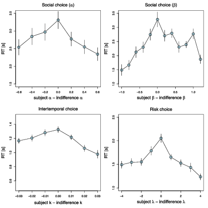
| Figure 1: RTs peak at indifference. Mean RT in seconds as a function of the
distance between the individual subject’s preference function parameter
and the indifference point on a particular trial; data are aggregated into
bins of width 0.02 (top row), 0.01 (bottom left panel), and 1 (bottom
right panel), which are truncated and centered for illustration purposes.
Bins with fewer than 10 subjects are removed for display purposes. Bars
denote standard errors, clustered at the subject level. |
Let us illustrate this concept with a simple example. Suppose that in the
intertemporal-choice task a subject has to choose between $25 today and
$40 in 30 days. The subject would be indifferent with an individual
discount rate k∗ that is the solution to the equation $25 =
$40/(1+30 k∗), or k∗ = 0.0125. This would be the
indifference point of this particular trial. A subject with k=k∗
would be indifferent on this trial, a subject with a k < k∗ would
favor the delayed option, and a subject with a higher k > k∗ would
favor the immediate option.
We hypothesized that the bigger the absolute difference between the
subject’s parameter and the trial’s indifference point |k−k∗|, the
stronger the preference, and the shorter the mean RT. This is analogous to
how, in decision field theory, the difference in valence between the two
options determines the preference state and thus the average speed of the
decision (Busemeyer & Townsend 1993). We observe this effect in all of our
datasets, with RTs peaking when a subject’s parameter is equal to the trial
indifference point (Figure 1). Mixed-effects regression models show
strong, statistically significant effects of the absolute distance between
the indifference point and subjects’ individual preference parameters on
log(RTs) for all the datasets (fixed effect of distance on RT: dictator
game α: t = −7.5, p < 0.001; dictator game β: t
= −9.1, p < 0.001; intertemporal choice k: t = −9.9, p
< 0.001; non-adaptive risky choice λ: t = −9.6, p
< 0.001, adaptive risky choice λ: t = −4.4, p
< 0.001).
Having verified the relationship between strength-of-preference and RT, we
next asked whether we could invert this relationship. In other words, we
sought to test whether one can estimate preferences from RTs. First, we
investigated whether RTs can reveal preference information when only a
single trial’s data is available.
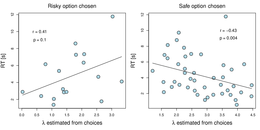
| Figure 2: Preference rank inferred from a single decision problem. RTs in
the first trial of the adaptive risk experiment as a function of the
individual subject’s loss-aversion coefficient from the whole experiment;
each point is a subject, Spearman correlations displayed. In this round,
each subject was presented with a binary choice between a lottery that
included a 50% chance of winning $12 and losing $7.5, and a sure option
of $0. The right panel displays subjects who chose the safe option, and
the left panel shows those who chose the risky option. The solid black
lines are regression model fits. |
3.2 One-trial preference ranking
In the adaptive risk experiment, all subjects faced the same choice problem
in the first trial. They had to choose between a 50/50 lottery with a
gain ($12) and a loss ($7.5), vs. a sure amount ($0).
Assuming risk neutrality, a subject with a loss aversion coefficient of
λ=1.6 should be indifferent between these two
options, with more loss-averse subjects picking the safe option, and the
rest picking the risky option.
Because the mean loss aversion (estimated based on all the
choices) in our sample was 2.5 (median = 2.46), most of the subjects (44
out of 61) picked the safe option in this first trial. Now, if we had to
restrict our experiment to just this one trial, the only way we could
classify subjects’ preferences would be to divide them into two groups:
those with λ ≥ 1.6 and those
with λ < 1.6. Within each group
we would not be able further distinguish between individuals.
However, by additionally observing RTs we can establish a ranking of the
subjects in each group. Specifically, we hypothesized that subjects with
loss aversion closer to 1.6 would exhibit longer RTs. To test this
hypothesis we ranked subjects in each group according to their RTs and then
compared those rankings to the “true” loss aversion parameters estimated
from all 30 choices in the full dataset (see Figure 2, Note 2 in the
Supplement, and Figure S5 for the choice-based estimates).
There was a significant rank correlation (Spearman) between RTs and
loss seeking in the “safe option” group (r = 0.43, p = 0.004) and
marginally between RTs and loss aversion in the “risky option” group (r =
0.41, p = 0.1). Thus, the single-trial RT-based rankings aligned quite
well with the 30-trial choice-based rankings.
3.3 Uninformative choices
A similar use of RT-based inference is the case where an experiment (or
questionnaire) is flawed in such a way that most subjects give the same
answer to the choice problem (e.g., because it has an extreme indifference
point, or because people feel social pressure to give a certain answer,
even if it contradicts their true preference (Coffman, Coffman &
Ericson, 2017)). This method could be used to bolster datasets that are
limited in scope and so unable to recover all subjects’ preferences.
To model this situation, for each dataset (non-adaptive risk, intertemporal
choice, and social choice) we isolated the 4–10 trials (depending on the
dataset) with the highest indifference points, where most subjects chose
the same option (e.g., the risky option), and limited our analysis to
those subjects who picked this most popular option. Then we iterated an
increasing set of trials (just the highest point, the first and the second
highest points, the first, second, and third, and so on), took the median
RT in this set, and correlated it with the “true” choice-based estimates.
We hypothesized that the slower the decisions on these trials, the more
extreme the choice-based parameter value for that subject.
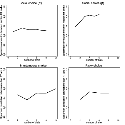
| Figure 3: Spearman correlations between choice-based parameter estimates
and the median RT in the trials with the highest indifference points, for
increasing sets of these extreme trials. |
The set of trials varied across datasets due to the structure of the
experiments. In the risk and intertemporal datasets every decision problem was shown
twice, so we started with two trials and then increased in steps of two.
For the risk task there were several trials with identical indifference
points after the first 8 trials, so we stopped there. For the
social-preference datasets there were many trials with the same
indifference point (8 and 6 for α and
β respectively) so we simply used those trials,
going from lowest to highest game id number (arbitrarily assigned in the
experiment code). Note that we used only the highest indifference points,
since trials with indifference parameters close to zero were often trivial
“catch” trials, e.g., $25 today vs. $25 in 7 days.
Confirming the hypothesis, we found that the RTs on these trials were
strongly predictive of subjects’ choice-based parameters in all four
domains (Figure 3), with Spearman correlations ranging from 0.37 to 0.84
(for the largest set: risk choice (n = 19): ρ =
0.50, p = 0.03; intertemporal choice (n = 25): ρ =
0.59, p = 0.002; social choice α (n = 26):
ρ = 0.50, p = 0.009; social choice
β (n = 20): ρ = 0.84, p
< 0.001). Thus, we again see, in every domain, that RT-based
rankings from a small subset of trials align well with choice-based
rankings from the full datasets. These analyses also hint at potential
benefits from including more trials, but also suggest that RTs may not be
that noisy once we control for the difficulty of the question and
subject-level heterogeneity.
3.4 DDM-based preference parameter estimation from RTs
The results described in the previous sections demonstrate that we can use
RT to rank subjects according to their preferences on trials where they
all make the same choice. A more challenging problem is to estimate a
subject’s preferences from RT alone. In this section, we explore ways to
estimate individual subjects’ preference parameters from their RTs across
multiple choice problems.
The DDM predicts more than just a simple relationship between
strength-of-preference and mean RT; it predicts entire RT distributions.
The drift rate in the model is a linear function of the subjective value
difference (or in decision field theory the valence difference) and so by
estimating drift rates we can potentially identify the latent preference
parameters. We hypothesized that the DDM-derived preference parameters,
using only RT data, would correlate with the choice-based preference
parameters estimated in the usual way.
We used the simple standard DDM, but did not condition the RT distributions
on the choice made in each trial (see Section 2.4. and the
Supplement). We assumed no starting point bias and,
following the traditional approach, assumed that the drift rate is a simple
linear function of the difference in subjective values (Busemeyer &
Townsend, 1993; Dai & Busemeyer, 2014). Parameter recovery simulations
confirmed that the preference parameters could be identified using this
method (Figure S6).
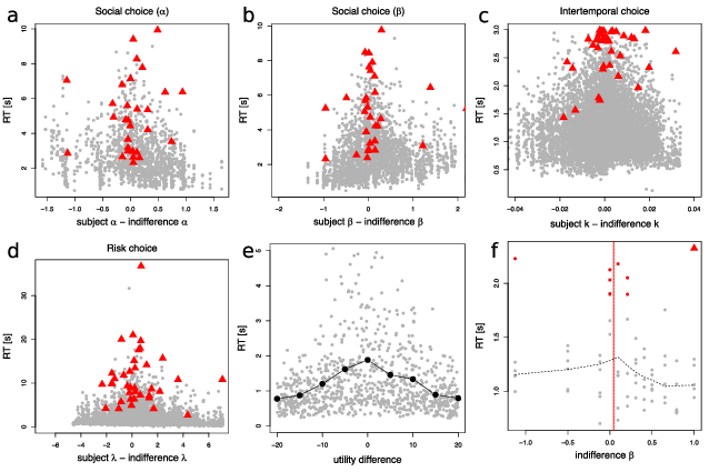
| Figure 4: Slow decisions tend to occur at indifference. (a-d) Subject data
from each task. RT in seconds as a function of the distance between the
individual subject preference parameter and the indifference point on a
particular trial; gray dots denote individual trials. Red triangles denote
trials with the highest RT for each individual subject. (e) Simulation of
the DDM. Response times (RTs) as a function of the difference in
utilities between two options in 900 simulated trials. The gray dots show
individual trials, the black circles denote averages with bins of width
10. The parameters used for the simulation correspond to the parameters
estimated at the group level in the time discounting experiment (b =
1.33, z = 0.09, τ = 0.11). Subjective-value
differences are sampled from a uniform distribution between −20 and 20.
(f) Example of an individual subject’s RT-based parameter estimation. The
plot shows RTs in all trials as a function of the indifference parameter
value on that trial. Observations in the top RT decile are shown in red.
The red triangle shows the longest RT for the subject. The solid vertical
red line shows the subject’s choice-based parameter estimate. The dotted
vertical red line shows the average indifference value for the top RT
decile approach. The dotted grey line shows the local regression fit
(LOWESS, smoothing parameter = 0.5). |
First, we estimated the DDM assuming that the boundary parameter b,
non-decision time τ, and drift scaling parameter z were fixed across
subjects (see Note 2 in the Supplement). We made this
simplifying assumption to drastically reduce the number of parameters we
needed to estimate. In each dataset, we found that DDM-derived preference
parameters were correlated with the choice-based parameters (social choice
α: r = 0.39, p = 0.04, t(27) = 2.2; social choice β: r = 0.52,
p = 0.003, t(28) = 3.2; intertemporal choice k: r = 0.57, p <
0.001, t(37) = 4.2; risky choice λ: r = 0.36, p = 0.03, t(35) =
2.26; Pearson correlations, Figure S7).
We did not use the adaptive risk dataset here (or for subsequent analyses)
since the adaptive nature of the task means that subjects should be closer
to indifference as the experiment progresses. The well-established
negative correlation between trial number and RT would thus counteract the
strength-of-preference effects and interfere with our ability to estimate
preferences.
We also estimated the DDM for each subject separately, assuming individual
variability in the boundary parameter b, non-decision time τ, and
drift scaling parameter z. In some cases, this causes identification
problems for certain subjects (the parameters were estimated at the bounds
of the possible range), most likely due to the small number of trials (only
48 trials to estimate 4 parameters in the case of α in the social
preference task) and the tight distribution of subjects’ indifference
points in that task. After excluding these subjects (2/30 and 2/30 in the
social choice dataset, 16/39 in the intertemporal choice dataset, and 7/37
in the risk choice dataset), we found that in most cases correlations
between DDM parameters and choice-based parameters were stronger than in
the pooled estimation variant (social choice α: r = 0.09, p = 0.65,
t(25) = 0.45; social choice β: r = 0.74, p < 0.001, t(26) =
5.54; intertemporal choice k: r = 0.63, p = 0.001, t(22) = 3.84; risky
choice λ: r = 0.53, p = 0.002, t(28) = 3.33; Pearson correlations,
Figure S8).
These results highlight that it is useful to have trials with a wide range
of indifference points. This can be inefficient with standard choice-based
analyses, since most subjects choose the same option on trials with extreme
indifference points. However, when including RTs, these trials can still
convey useful information, namely the strength-of-preference.
3.5 Alternative approaches to preference parameter estimation from RTs
The DDM may seem optimal for parameter recovery if that is indeed the data
generating process. However, several factors likely limit its usefulness
in our settings. The DDM has several free parameters that are identified
using features of choice-conditioned RT distributions. Identification
thus typically relies on many trials and observing choice outcomes.
Without meeting these two requirements, the DDM approach may struggle to
identify parameters accurately. Thus, we explored alternative, simpler
approaches to analyzing the RTs.
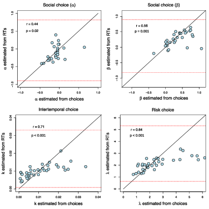
| Figure 5: Estimates of subjects’ preference parameters, estimated using the
top RT decile method. Subject-level correlation (Pearson) between
parameters estimated from choice data and RT data. The solid lines are 45
degree lines. The dotted red lines indicate the minimum and maximum
parameter values that can be estimated from the RTs. |
One alternative approach is to focus on the longest RTs. Long RTs are
considerably more informative than short RTs. Sequential sampling models
correctly predict that short RTs can occur at any level of
strength-of-preference, but long RTs almost exclusively occur near
indifference (Figure 4). With these facts in mind, we set about
constructing an alternative method for using RTs to infer a subject’s
indifference point. Clearly, focusing on the slowest trials would yield
less biased estimates of subjects’ indifference points. However, using
too few slow trials would increase the variance of those estimates. We
settled on a simple method that uses the slowest 10% of a subject’s
choices, though we also explored other cutoffs (Figure S9).
In short, our estimation algorithm for an individual subject includes the
following steps: (1) identify trials with RTs in the upper 10% (the
slowest decile); (2) for each of these trials, calculate the value of the
preference parameter that would make the subject indifferent between the
two alternatives; (3) average these values to get the estimate of the
subject’s parameter (see Figure 4f and the Supplement for
formal estimation details and Figure S6 for the parameter recovery
simulations). It is important to note that this method puts bounds on
possible parameter estimates: the average of the highest 10% of all
possible indifference values is the upper bound, while the average of the
lowest 10% of the indifference values is the lower bound.
Again, the parameters estimated using this method were correlated with the
same parameters estimated purely from the choice data, providing a better
prediction than the DDM approach (social choice α:
r = 0.44, p = 0.02, t(27) = 2.54; social choice β:
r = 0.56, p = 0.001, t(28) = 3.57; intertemporal choice k: r = 0.71, p
< 0.001, t(37) = 6.17; risky choice λ:
r = 0.64, p < 0.001, t(35) = 4.9; Pearson correlations; Figure
5, see the Supplement for estimation details for both methods).
Furthermore, these parameters provided prediction accuracy that was better
than the informed baseline in three out of four cases (excluding social
choice α). In all cases, a random 10% sample of
trials produced estimates that were not a meaningful predictor of the
choice-based parameter values (since these estimates are just a mean of
10% random indifference points). The RT-based estimations have upper and
lower bounds due to averaging over a 10% sample of trials and thus are
not able to capture some outliers (Figure 5). Furthermore, the number of
“extreme” indifference points in the choice problems that we considered is
low, biasing the RT-based estimates towards the middle.
We also explored a method using the whole set of RT data and a
non-parametric regression, but its performance was uneven across the
datasets (see the Supplement and Figure S6 for the parameter
recovery).
3.6 Choice reversals
Finally, we explored one additional set of predictions from the revealed
strength-of-preference approach. We know that when subjects are closer to
indifference, their choices become less predictable, and they slow down.
Therefore, slow choices should be less likely to be repeated (Alós-Ferrer
et al., 2016).
In all three datasets, the choice-estimated preference model was
significantly less consistent with long-RT choices than with short-RT
choices (based on a median split within subject): 80% vs 89% (p
< 0.001) in the risky choice experiment, 71% vs 79% (p
< 0.001) in the intertemporal choice experiment, 88% vs 94% (p
= 0.008) and 90% vs 96% (p < 0.001) in the dictator game
experiment; p-values denote Wilcoxon signed rank test significance on the
subject level.
A second, more nuanced feature of DDMs is that with typical parameter
values, without time pressure, they sometimes predict “slow errors”, even
conditioning on difficulty (Ratcliff & McKoon, 2008). In preferential
choice there are no clear correct or error responses, however, we can
compare choices that are consistent or inconsistent with the best-fitting
choice model. The prediction is that inconsistent choices should be
slower than consistent ones.
To control for choice difficulty, we ran mixed-effects regressions of
choice consistency on the RTs and the absolute subjective-value difference
between the two options. In all cases we found a strong negative
relationship between the RTs and the choice consistency (slower choice =
less consistent) (fixed effects of RTs: social choice
α: z = −2.62, p = 0.009; social choice
β: z = −3.3, p < 0.001, intertemporal
choice: z = −5.28, p < 0.001, risk choice: z = −5.35, p
< 0.001).
In two of the datasets (intertemporal choice and non-adaptive risk choice)
subjects faced the same set of decision problems twice. This allowed us to
perform a more direct test of the slow inconsistency hypothesis by seeing
whether slow decisions in the first encounter were more likely to be
reversed on the second encounter.
In the intertemporal choice experiment, the median RT for a later-reversed
decision was 1.36 s, compared to 1.17 s for a later-repeated decision. A
mixed-effects regression effect of first-choice RT on choice reversal,
controlling for the absolute subjective-value difference, was highly
significant (z = 4.04, p < 0.001). The difference was even
stronger in the risk choice experiment: subsequently reversed choices took
2.36 s versus only 1.4 s for subsequently repeated choices. Again, a
mixed-effects regression revealed that RT was a significant predictor of
subsequent choice reversals (controlling for absolute subjective-value
difference, z = 5.2, p < 0.001).
There are a couple of intuitions for why slow decisions are still less
consistent, even after controlling for difficulty. First, the true
difficulty of a decision can only be approximated. Even with identical
choice problems, one attempt at that decision might be more subjectively
difficult than another. In the DDM, this is captured by across-trial
variability in drift rate. In other words, one cannot fully control for
difficulty in these kinds of analyses. So, slow decisions can still
signal proximity to indifference, and thus inconsistency in choice.
Second, slow errors can also arise from starting-points that are biased
towards the preferred category (e.g., risky options) (Chen & Krajbich,
2018; White & Poldrack, 2014). In these cases, preference-inconsistent
choices typically have longer distances to cover during the diffusion
process and so take more time.
4 Discussion
Here we have demonstrated a proof-of-concept for the method of revealed
strength-of-preference. This method contrasts with the standard method of
revealed preference, by using response times (RTs) rather than choices to
infer preferences. It relies on the fact that people generally take
longer to decide as they approach indifference. Using datasets from three
different choice domains (risk, temporal, and social) we established that
preferences are highly predictable from RTs alone. Finally, we also found
that long RTs are predictive of choice errors, as captured by
inconsistency with the estimated preference function and later choice
reversals.
Our findings also have important implications for anyone who studies
individual preferences.
First, using RTs may allow one to estimate subjects’ preferences using very
short and simple decision tasks, even a single binary-choice problem.
This is important since researchers, and particularly practitioners, can
often only record a small number of decisions (Toubia, Johnson, Evgeniou
& Delquié, 2013). Since RT data is easily available in online
marketplaces, and many purchases or product choices occur only once, these
data might provide important insight into customers’ preferences. Along
the way, the speed with which customers reject other products might also
reveal important information. On the other hand, clients who wish to
conceal their strength-of-preference, might use their RT strategically to
avoid revealing their product valuations.
Second, the fact that RTs can be used to infer preferences when choices are
unobservable or uninformative is an important point for those who are
concerned about private information, institution design, etc. For
instance, while voters are very concerned about the confidentiality of
their choices, they may not be thinking about what their time in the
voting booth might convey about them. In an election where most of a
community’s voters strongly favor one candidate, a long stop in the voting
booth may signal dissent. Another well-known example is the implicit
association test (IAT), where subjects’ RTs are used to infer personality
traits (e.g., racism) that the subjects would otherwise not admit to or
even be aware of (Greenwald, McGhee & Schwartz, 1998). Thus, protecting
privacy may involve more than simply masking choice outcomes.
Third, our work highlights a method for detecting choice errors. While the
standard revealed preference approach must equate preferences and choices,
the revealed strength-of-preference approach allows us to identify choices that are
more likely to have been errors, or at the very least, made with low
confidence.
There are of course limitations to using RTs to infer strength-of-preference. Other
factors may influence RTs in addition to strength-of-preference, such as
complexity, stake size, and trial number (Krajbich, Hare, Bartling & Fehr, 2015; Logan,
1992; Moffatt, 2005). It may be important to account for these factors in
order to maximize the chance of success. A second issue is that we have
focused on repeated decisions which are made quite quickly (1–3 seconds on
average) and so the results may not necessarily extend to slower, more
complex decisions (but see Krajbich, Hare, Bartling & Fehr, 2015).
More research is required to distinguish between SSMs and alternative
frameworks (Achtziger & Alós-Ferrer, 2013; Alós-Ferrer et al., 2016;
Alós-Ferrer & Ritschel, 2018; Hey, 1995; Kahneman, 2013; Rubinstein,
2016), where long RTs are associated with more careful or deliberative
thought and short RTs are associated with intuition. It may in fact be
the case that in some instances people do use a logic-based approach, in
which case a long RT may be more indicative of careful thought, while in
other instances they rely on a SSM approach, in which case a long RT
likely indicates indifference. This could lead to contradictory
conclusions from the same RT data; for example, one researcher may see a
long RT and assume the subject is very well informed, while another
researcher may see that same RT and assume the subject has no evidence one
way or the other. More research is required to test whether SSMs, which
are designed to tease apart such explanations, can be successfully applied
to complex decisions.
5 References
Achtziger, A., & Alós-Ferrer, C. (2013). Fast or rational? A
response-times study of Bayesian updating. Management Science,
60(4), 923–938.
Ainslie, G. (1992). Picoeconomics: The strategic interaction of
successive motivational states within the person. Cambridge University
Press.
Alós-Ferrer, C., Granić, Ð.-G., Kern, J., & Wagner, A. K. (2016).
Preference reversals: Time and again. Journal of Risk and
Uncertainty, 52(1), 65–97.
Alós-Ferrer, C., & Ritschel, A. (2018). The reinforcement heuristic in
normal form games. Journal of Economic Behavior & Organization,
152, 224–234.
Amasino, D. R., Sullivan, N. J., Kranton, R. E., & Huettel, S. A. (2019).
Amount and time exert independent influences on intertemporal choice.
Nature Human Behaviour. https://doi.org/10.1038/s41562-019-0537-2
Bergert, F. B., & Nosofsky, R. M. (2007). A response-time approach to
comparing generalized rational and take-the-best models of decision
making. Journal of Experimental Psychology: Learning, Memory, and
Cognition, 33(1), 107.
Bhatia, S., & Mullett, T. L. (2018). Similarity and decision time in
preferential choice. Quarterly Journal of Experimental
Psychology, 1747021818763054.
Bogacz, R., Brown, E., Moehlis, J., Holmes, P., & Cohen, J. D. (2006). The
physics of optimal decision making: A formal analysis of models of
performance in two-alternative forced choice tasks. Psychological
Review, 113(4), 700–765.
Brunton, B. W., Botvinick, M. M., & Brody, C. D. (2013). Rats and humans
can optimally accumulate evidence for decision-making. Science,
340, 95–98.
Busemeyer, J. R. (1985). Decision making under uncertainty: A comparison of
simple scalability, fixed-sample, and sequential-sampling models.
Journal of Experimental Psychology: Learning, Memory, and
Cognition, 11(3), 538–564.
https://doi.org/10.1037/0278-7393.11.3.538
Busemeyer, J. R., & Rapoport, A. (1988). Psychological models of deferred
decision making. Journal of Mathematical Psychology, 32,
91–134.
Busemeyer, J. R., & Townsend, J. T. (1993). Decision field theory: A
dynamic-cognitive approach to decision making in an uncertain environment.
Psychological Review, 100(3), 432–459.
Caplin, A., & Martin, D. (2016). The dual-process drift diffusion model:
evidence from response times. Economic Inquiry, 54(2),
1274–1282. https://doi.org/10.1111/ecin.12294
Chabris, C. F., Morris, C. L., Taubinsky, D., Laibson, D., & Schuldt, J.
P. (2009). The allocation of time in decision-making. Journal of
the European Economic Association, 7(2–3), 628–637.
Chapman, J., Snowberg, E., Wang, S., & Camerer, C. (2018). Loss attitudes
in the U.S. population: Evidence from dynamically optimized sequential
experimentation (DOSE). National Bureau of Economic Research
Working Paper Series, No. 25072. https://doi.org/10.3386/w25072
Chen, F., & Krajbich, I. (2018). Biased sequential sampling underlies the
effects of time pressure and delay in social decision making.
Nature Communications, 9(1), 3557.
https://doi.org/10.1038/s41467-018-05994-9.
Cleveland, W. S. (1979). Robust locally weighted regression and smoothing
scatterplots. Journal of the American Statistical Association,
74(368), 829–836.
Clithero, J. A. (2018). Improving Out-of-Sample Predictions. Using Response
Times and a Model of the Decision Process. Journal of Economic
Behavior & Organization. https://doi.org/10.1016/j.jebo.2018.02.007.
Coffman, K. B., Coffman, L. C., & Ericson, K. M. M. (2017). The size of
the LGBT population and the magnitude of antigay sentiment are
substantially underestimated. Management Science,
63(10), 3168–3186. https://doi.org/10.1287/mnsc.2016.2503.
Dai, J., & Busemeyer, J. R. (2014a). A probabilistic, dynamic, and
attribute-wise model of intertemporal choice. Journal of
Experimental Psychology: General, 143(4), 1489–1514.
https://doi.org/10.1037/a0035976.
Dashiell, J. F. (1937). Affective value-distances as a determinant of
esthetic judgment-times. The American Journal of Psychology.
De Martino, B., Fleming, S. M., Garret, N., & Dolan, R. J. (2013).
Confidence in value-based choice. Nature Neuroscience,
16(1), 105–110.
Diederich, A. (1997). Dynamic stochastic models for decision making under
time constraints. Journal of Mathematical Psychology,
41(3), 260–274. https://doi.org/10.1006/jmps.1997.1167.
Diederich, A. (2003). MDFT account of decision making under time pressure.
Psychonomic Bulletin & Review, 10(1), 157–166.
https://doi.org/10.3758/BF03196480.
Echenique, F., & Saito, K. (2017). Response time and utility.
Journal of Economic Behavior & Organization, 139,
49–59.
Fehr, E., & Schmidt, K. M. (1999). A theory of fairness, competition, and
cooperation. The Quarterly Journal of Economics, 114(3),
817–868.
Fiedler, S., & Glöckner, A. (2012). The dynamics of decision making in
risky choice: An eye-tracking analysis. Frontiers in Psychology,
3. https://doi.org/10.3389/fpsyg.2012.00335.
Fific, M., Little, D. R., & Nosofsky, R. M. (2010). Logical-rule models of
classification response times: A synthesis of mental-architecture,
random-walk, and decision-bound approaches. Psychological Review,
117(2), 309.
Fudenberg, D., Strack, P., & Strzalecki, T. (2018). Speed, accuracy, and
the optimal timing of choices. American Economic Review,
108(12), 3651–3684.
Gabaix, X., Laibson, D., Moloche, G., & Weinberg, S. (2006). Costly
Information Acquisition: Experimental Analysis of a Boundedly Rational
Model. American Economic Review, 96(4), 1043–1068.
https://doi.org/10.1257/aer.96.4.1043.
Greenwald, A. G., McGhee, D. E., & Schwartz, J. L. (1998). Measuring
individual differences in implicit cognition: the implicit association
test. Journal of Personality and Social Psychology,
74(6), 1464.
Hare, T. A., Hakimi, S., & Rangel, A. (2014). Activity in dlPFC and its
effective connectivity to vmPFC are associated with temporal discounting.
Frontiers in Neuroscience, 8.
https://doi.org/10.3389/fnins.2014.00050.
Haxby, J. V., Connolly, A. C., & Guntupalli, J. S. (2014). Decoding neural
representational spaces using multivariate pattern analysis.
Annual Review of Neuroscience, 37, 435–456.
Hey, J. D. (1995). Experimental investigations of errors in decision making
under risk. European Economic Review, 39(3), 633–640.
Hunt, L. T., Kolling, N., Soltani, A., Woolrich, M. W., Rushworth, M. F.
S., & Behrens, T. E. (2012). Mechanisms underlying cortical activity
during value-guided choice. Nature Neuroscience, 15,
470–476.
Hutcherson, C. A., Bushong, B., & Rangel, A. (2015). Al neurocomputational
model of altruistic choice and its implications. Neuron,
87(2), 451–462.
Jamieson, D. G., & Petrusic, W. M. (1977). Preference and the time to
choose. Organizational Behavior and Human Performance,
19(1), 56–67.
Kahneman, D. (2013). Thinking, Fast and Slow (Reprint edition).
New York: Farrar, Straus and Giroux.
Kahneman, D., & Tversky, A. (1979). Prospect theory: an analysis of
decision under risk. Econometrica, 4, 263–291.
Konovalov, A., & Krajbich, I. (2016). Gaze data reveal distinct choice
processes underlying model-based and model-free reinforcement learning.
Nature Communications, 7, 12438.
Krajbich, I., Armel, K. C., & Rangel, A. (2010). Visual fixations and the
computation and comparison of value in simple choice. Nature
Neuroscience, 13(10), 1292–1298.
Krajbich, I., Bartling, B., Hare, T., & Fehr, E. (2015). Rethinking fast
and slow based on a critique of reaction-time reverse inference.
Nature Communications, 6, 7455.
https://doi.org/10.1038/ncomms8455.
Krajbich, I., Hare, T., Bartling, B., Morishima, Y., & Fehr, E. (2015). A
common mechanism underlying food choice and social decisions. PLoS
Computational Biology, 11(10), e1004371
Krajbich, I., & Rangel, A. (2011). Multialternative drift-diffusion model
predicts the relationship between visual fixations and choice in
value-based decisions. Proceedings of the National Academy of
Sciences, 108(33), 13852–13857.
Laibson, D. (1997). Golden eggs and hyperbolic discounting. The
Quarterly Journal of Economics, 443–477.
Loewenstein, G., & Prelec, D. (1992). Anomalies in intertemporal choice:
Evidence and an interpretation. The Quarterly Journal of
Economics, 107(2), 573–597.
Logan, G. D. (1992). Shapes of reaction-time distributions and shapes of
learning curves: A test of the instance theory of automaticity.
Journal of Experimental Psychology: Learning, Memory, and
Cognition, 18(5), 883.
Loomes, G. (2005). Modelling the stochastic component of behaviour in
experiments: Some issues for the interpretation of data.
Experimental Economics, 8, 301–323.
Luce, R. D. (1986). Response Times: Their Role in Inferring
Elementary Mental Organization. Oxford: Oxford University Press.
Milosavljevic, M., Malmaud, J., Huth, A., Koch, C., & Rangel, A. (2010).
The drift diffusion model can account for the accuracy and reaction time
of value-based choices under high and low time pressure. Judgment
and Decision Making, 5(6), 437–449.
Moffatt, P. G. (2005). Stochastic choice and the allocation of cognitive
effort. Experimental Economics, 8(4), 369–388.
Mosteller, F., & Nogee, P. (1951). An experimental measurement of utility.
Journal of Political Economy, 59(5), 371–404.
Polanía, R., Krajbich, I., Grueschow, M., & Ruff, C. C. (2014). Neural
Oscillations and Synchronization Differentially Support Evidence
Accumulation in Perceptual and Value-Based Decision Making.
Neuron, 82(3), 709–720.
https://doi.org/10.1016/j.neuron.2014.03.014.
Ratcliff, R., & McKoon, G. (2008). The diffusion decision model: Theory
and data for two-choice decision tasks. Neural Computation,
20(4), 873–922.
Rodriguez, C. A., Turner, B. M., & McClure, S. M. (2014). Intertemporal
choice as discounted value accumulation. PloS One, 9(2),
e90138.
Roe, R. M., Busemeyer, J. R., & Townsend, J. T. (2001). Multialternative
decision field theory: A dynamic connectionist model of decision making.
Psychological Review, 108(2), 370–392.
Rubinstein, A. (2007). Instinctive and cognitive reasoning: A study of
response times. The Economic Journal, 117(523),
1243–1259.
Rubinstein, A. (2016). A typology of players: Between instinctive and
contemplative. The Quarterly Journal of Economics,
131(2), 859–890.
Samuelson, P. A. (1938). A note on the pure theory of consumer’s behaviour.
Economica, 5(17), 61–71.
Shadlen, M. N., & Shohamy, D. (2016). Decision Making and Sequential
Sampling from Memory. Neuron, 90(5), 927–939.
https://doi.org/10.1016/j.neuron.2016.04.036.
Sokol-Hessner, P., Hsu, M., Curley, N. G., Delgado, M. R., Camerer, C. F.,
& Phelps, E. A. (2009). Thinking like a trader selectively reduces
individuals’ loss aversion. Proceedings of the National Academy of
Sciences, 106(13), 5035–5040.
Spiliopoulos, L., & Ortmann, A. (2017). The BCD of response time analysis
in experimental economics. Experimental Economics.
https://doi.org/10.1007/s10683-017-9528-1.
Stewart, N., Hermens, F., & Matthews, W. J. (2015). Eye Movements in Risky
Choice: Eye Movements in Risky Choice. Journal of Behavioral
Decision Making, 29(2-3),116-136. https://doi.org/10.1002/bdm.1854.
Tajima, S., Drugowitsch, J., & Pouget, A. (2016). Optimal policy for
value-based decision-making. Nature Communications, 7,
12400. https://doi.org/10.1038/ncomms12400.
Toubia, O., Johnson, E., Evgeniou, T., & Delquié, P. (2013). Dynamic
experiments for estimating preferences: An adaptive method of eliciting
time and risk parameters. Management Science, 59(3),
613–640.
Tversky, A., & Shafir, E. (1992). Choice under conflict: The dynamics of
deferred decision. Psychological Science, 3(6), 358–361.
Usher, M., & McClelland, J. (2001). The time course of perceptual choice:
The leaky, competing accumulator model. Psychological Review,
108(3), 550–592.
Wabersich, D., & Vandekerckhove, J. (2014). The RWiener package: An R
package providing distribution functions for the Wiener diffusion model.
R Journal, 6(1).
White, C. N., & Poldrack, R. A. (2014). Decomposing bias in different
types of simple decisions. Journal of Experimental Psychology:
Learning, Memory, and Cognition, 40(2), 385.
Wilcox, N. T. (1993). Lottery choice: Incentives, complexity and decision
time. The Economic Journal, 1397–1417.
Woodford, M. (2014). Stochastic Choice: An Optimizing Neuroeconomic Model.
American Economic Review, 104(5), 495–500.
https://doi.org/10.1257/aer.104.5.495.
This document was translated from LATEX by
HEVEA.