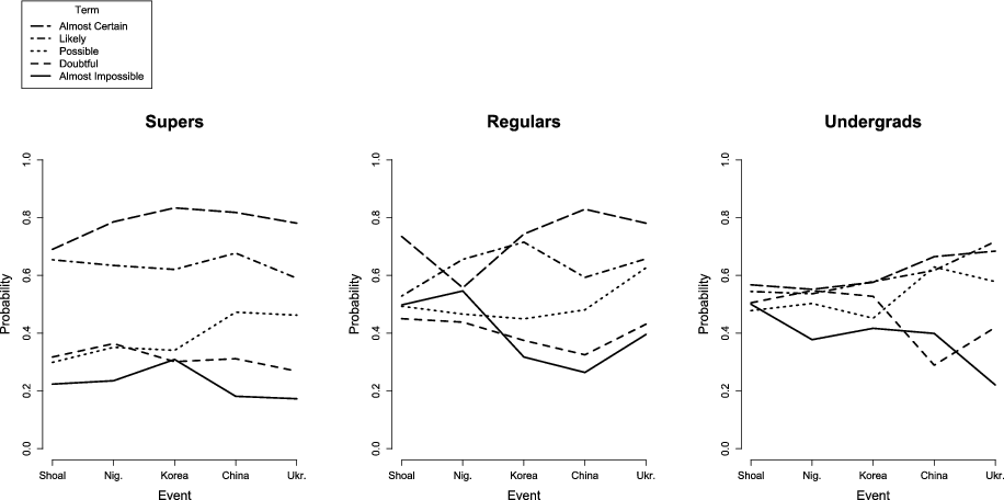
 Figure 1: Average numerical interpretation of probability phrases in survey 1.
Judgment and Decision Making, Vol. 12, No. 4, July 2017, pp. 369-381
How generalizable is good judgment? A multi-task, multi-benchmark studyBarbara A. Mellers* Joshua D. Baker# Eva Chen# David R. Mandel$ Philip E. Tetlock$ |
Good judgment is often gauged against two gold standards – coherence and correspondence. Judgments are coherent if they demonstrate consistency with the axioms of probability theory or propositional logic. Judgments are correspondent if they agree with ground truth. When gold standards are unavailable, silver standards such as consistency and discrimination can be used to evaluate judgment quality. Individuals are consistent if they assign similar judgments to comparable stimuli, and they discriminate if they assign different judgments to dissimilar stimuli. We ask whether “superforecasters”, individuals with noteworthy correspondence skills (see Mellers et al., 2014) show superior performance on laboratory tasks assessing other standards of good judgment. Results showed that superforecasters either tied or out-performed less correspondent forecasters and undergraduates with no forecasting experience on tests of consistency, discrimination, and coherence. While multifaceted, good judgment may be a more unified than concept than previously thought.
Keywords:
Social scientists and philosophers often evaluate judgments against two gold standards: correspondence and coherence (Hammond, 1996, 2007). Measures of correspondence capture the degree to which judgments agree with empirical observations (e.g., Cooksey, 1996; Hammond, 1996), and coherence criteria assess the degree to which judgments are consistent with logical or axiomatic principles. Both standards are widely accepted as important components of good judgment (Dunwoody & College, 2009; Hammond, 2000).
Previous research suggests that human judgment tends to fall short on coherence and correspondence. Coherence violations range from base rate neglect and confirmation bias to overconfidence and framing effects (Gilovich, Griffith & Kahneman, 2002; Kahneman, Slovic & Tversky, 1982). Experts are not immune. Statisticians (Christensen-Szalanski & Bushyhead, 1981), doctors (Eddy, 1982), and nurses (Bennett, 1980) neglect base rates. Physicians and intelligence professionals are susceptible to framing effects (Aberegg, Arkes & Terry, 2006; Reyna, Chick, Corbin & Hsia, 2014), and financial investors are prone to overconfidence (Barber & Odean, 2001).
Research on correspondence tells a similar story. Numerous studies show that human predictions are frequently inaccurate and worse than simple linear models in many domains (e.g., Meehl, 1954; Dawes, Faust & Meehl, 1989). Once again, expertise doesn’t necessarily help. Inaccurate predictions have been found in parole officers (Carroll & Payne, 1977), court judges (Ebbesen & Konecki, 1975), investment managers in the US and Taiwan (Olsen, 1997), and politicians (Tetlock, 2005). However, expert predictions are better when the forecasting environment provides regular, clear feedback and there are repeated opportunities to learn (Kahneman & Klein, 2009; Shanteau, 1992). Examples include meteorologists (Murphy & Winkler, 1984), professional bridge players (Keren, 1987), and bookmakers at the racetrack (Bruce & Johnson, 2003), all of whom are well-calibrated in their own domains.
In many cases, judgment quality is important, but gold standards are unavailable. How “good” is a physician’s diagnosis, for example? Or an instructor’s grade, or a judge’s sentencing decision? Einhorn (1972, 1974), and Weiss & Shanteau (2003) suggested that, at a minimum, good judges (i.e., domain experts) should demonstrate consistency and discrimination in their judgments. In other words, experts should make similar judgments if cases are alike, and dissimilar judgments when cases are unalike. Indeed, some would argue that these skills are essential to expertise.
In a test of the consistency, Skånér, Strender & Bring (1998) asked 27 general practitioners (GPs) to estimate the probability of patient heart failure from a series of vignettes based on actual patients. In the vignettes, GPs were given diagnostic cues such as age, sex, and history of myocardial infarction, but the patients’ eventual survival status could not be obtained. GPs were presented with 45 cases, five of which were presented twice, and consistency was operationalized as the absolute difference in survival estimates on the five repeated cases. Individual consistency varied greatly. Absolute differences fell between 0 and 10% in 62% of cases, 11% to 20% in 25% of cases, and greater than 20% in 13% of cases. In another test of consistency, Dhami & Ayton (2001) found inconsistency in magistrate’s decisions across repeated trials in a laboratory task of bail setting.
We know of no studies that have examined good judgment using all four of the standards. One study examined three of them (Weiss, Brennan, Thomas, Kirlik & Miller, 2009). Using a golf putting task with experienced golfers, they found a strong correlation between accuracy and their combined measure of consistency and discrimination.
In a handful of studies, researchers have investigated connections between the gold standards, but results have been mixed. Most studies show weak connections (Wright & Ayton, 1987a; 1987b; Wright, Rowe, Bolger & Gammack, 1994; Adam & Reyna, 2005; Weaver & Stewart, 2012; Dunwoody et al., 2005), although one could argue that Weiss et al.’s results are an exception. For the most part, however, measures of coherence and correspondence are loosely coupled.
Yet under the right conditions, loose couplings may tighten. In research on forecasting, for example, some studies have given subjects a battery of coherence tasks prior to having them make forecasts about uncertain events. The results show that aggregate forecasts are more accurate (i.e., more correspondent) when subjects’ predictions are weighted by their scores on the coherence tasks, rather than combined with a simple unweighted average. Indeed, coherence-based weighting schemes have been shown to improve the accuracy of the aggregate by more than 30%, relative to a simple mean (Predd, Osherson, Kulkarni & Poor, 2008; Wang Kulkarni, Poor & Osherson, 2011; Tsai & Kirlik, 2012; Karvetski, Olson, Mandel & Twardy, 2013). Perhaps correspondence and coherence are intertwined, but we’ve been looking in the wrong places.
In previous research, we have examined a group of individuals with remarkable correspondence skills in geopolitical forecasting. These individuals were identified over the course of four geopolitical forecasting tournaments sponsored by the Intelligence Advanced Research Projects Activity (IARPA), the research and development wing of the U.S. intelligence community (Mellers, Stone, Murray, Minster, Rohrbaugh, Bishop, Chen, Baker, Hou, Horowitz, Ungar & Tetlock, 2015a; Tetlock & Gardner, 2015). In these tournaments, thousands of people predicted the outcomes of questions such as “Will the U.N General Assembly recognize a Palestinian state by September, 30, 2011?” Each year, the top 2% of subjects were designated “superforecasters” and were assigned to work together in elite teams. In this richer setting, superforecasters became more accurate and resisted regression to the mean, suggesting that their accuracy was driven at least in part by skill, rather than luck (Mellers, Stone, Atanasov, Rohrbaugh, Metz, Ungar, Bishop, Horowitz, Merkle & Tetlock, 2015b). Indeed, using Brier scores to measured accuracy, Goldstein, Hartman, Comstock and Baumgarten (2016) found that superforecasters outperformed U.S. intelligence analysts on the same questions by roughly 30%.
Who were these remarkable individuals? Superforecasters were well-educated, all having at least college degrees, and about two thirds with post-graduate degrees. They came from a diverse range of fields, including law, pharmacy, biochemistry, photography, computer science, venture capitalism, and mathematics. Some had training in probability and statistics, but none were subject matter experts because the range of topics in the tournaments was too great for any person to master singlehandedly. One could say that superforecasters were better characterized as super-generalists than as subject matter experts (Tetlock & Gardner, 2015).
What explained superforecasters’ success? Several hypotheses are supported (Mellers et al., 2015a). First, superforecasters were more actively open-minded and had greater fluid and crystallized intelligence than the average forecaster. Second, they were more motivated, as measured by the number of questions they attempted and the rate at which they updated their predictions. Third, they acquired task-specific skills, including scope sensitivity, which is the calibration of probabilities across regional, temporal, and quantitative dimensions (Mellers, et al., 2015a). They also expressed their beliefs in a more nuanced way by making more distinctions on the probability scale than other forecasters (Friedman, Baker, Mellers, Tetlock & Zeckhauser, 2017). Fourth, superforecasters, who always worked in teams, had more stimulating environments than others. Compared to regular teams, superforecaster shared more information, engaged in more discussions, offered more encouragement, and conducted more in-depth post mortems to gain insights from their successes and failures.
We ask a question that follows naturally from the forecasting tournaments discussed earlier. Are superforecasters, who were markedly better on measures of correspondence than their peers, also better on other standards of good judgment, including consistency, discrimination, and coherence? We use data from two online surveys to compare the judgments of superforecaters to those made by a less elite group of forecasters (hereafter called “regular” forecasters) and University of Pennsylvania undergraduates. Regular forecasters participated in the same tournaments as superforecasters, but were not as accurate, received no training in probabilistic reasoning, and worked alone rather than in teams. Undergraduates had no experience with forecasting at all.
There are numerous ways to assess each standard of judgment. We evaluated consistency and discrimination using a task from an early experiment by Wallsten, Budescu, Rapoport, Zwick & Forsyth (1986). Wallsten et al.’s subjects assigned numerical values to verbal uncertainty phrases such as “likely”, “unlikely”, and “possible”. Subjects showed widespread individual differences in their numerical interpretations of the phrases. Moreover, when the uncertainty phrases were paired with events, numerical interpretations varied even more (Cohen, 1986; Mandel, 2015). A “good chance” of having cancer, for example, was judged as likelier than a “good chance” of rain. We will measure consistency using a similar task. We’ll focus on the extent to which probability phrases are influenced by events. We’ll measure discrimination by computing the difference in numerical estimates for the most extreme probability phrases.
Coherence is often assessed using Bayesian reasoning problems (Kahneman & Tversky, 1985; Gigerenzer & Hoffrage, 1995). We used these problems, but also included questions about information needed for updating one’s beliefs, questions about which of two pieces of information is more diagnostic, and questions about whether to use normatively useless information.
The questions about information needed to update one’s beliefs come from a pseudodiagnosticity task developed by Doherty, Mynatt, Tweney and Schiavo (1979). Subjects read about an undersea explorer who found a valuable pot and wanted to return it to its place of origin – either Coral Island or Shell Island. The pot had smooth (vs. rough) clay and a curved (vs. straight) handle. Subjects were asked which information they most wanted to see from a limited set of probabilities. Not being Bayesians, subjects often selected nondiagnostic pairs of information. We also used questions from Baron, Beattie and Hershey (1988) about congruence and information biases. The congruence bias is a preference for less diagnostic information if that information is more likely to give a positive result for the favored hypothesis, and the information bias is a preference for more information, even if it will not change the decision.
Table 1: Laboratory tasks and associated benchmarks across the two surveys.
Survey 1 Survey 2 Consistency Verbal Uncertainty (I) Verbal Uncertainty (II) Main effect of event Main effect of event Avg. width of plausible intervals Avg. width of plausible intervals Discrimination Verbal Uncertainty (I) Verbal Uncertainty (II) Difference between extreme terms Difference between extreme terms [Main effect of probability phrase]** [Main effect of probability phrase] Coherence Pseudodiagnosticity Bayesian Updating Number of diagnostic item-pairs selected Prop. of correct responses (± 1%) Cognitive Bias Tasks Avg. absolute error across questions Congruence bias question Information bias question * See footnote 1
Following from the conjecture that expertise moderates the strength of the relationships among gold- and silver-standards of good judgment, we propose that the skills required to excel on correspondence tasks might also manifest themselves in performance on other benchmarks. Consequently, we predicted that superforecasters would be more coherent, more consistent, and better able to discriminate than other groups of subjects. Similarly, we expected regular forecasters to have acquired some degree of expertise with correspondence skills (but perhaps not as much), and undergraduates to have acquired less expertise still. Thus, we expected that regular forecasters would perform second best on the judgment tasks, and that undergraduates would perform the worst. Obviously, our laboratory tasks are only a small set of the possible ways we could assess good judgment, and groups could be equally skilled at some of them. In sum, our hypothesis was that superforecasters would perform at least as well as comparison groups on tasks of consistency, discrimination, or coherence.
We administered two surveys, six months apart. Table 1 shows a summary of the relevant tasks in each survey that are discussed in greater detail below. In both surveys, tasks were presented in the order shown in Table 1.
In the first survey, responses were obtained from 173 superforecasters (69% response rate); 75 regular forecasters (48% response rate); and 92 undergraduates. In the second survey, responses were obtained from 67 superforecasters (52% response rate); 90 regular forecasters (47% response rate); and 186 undergraduates. Some forecasters participated in both surveys. They included 52 superforecasters and 35 regular forecasters. Forecasters were, on average, 37.1 years (SD = 8.3) old, and all of them had at least a Bachelors’ degree. Undergraduates were, on average, 19.7 years old (SD = 0.8), and none of them had acquired college degrees.
Forecasters were rewarded with an electronic book upon the completion of each survey. Undergraduates were recruited by the Wharton Behavioral Lab at the University of Pennsylvania, and were paid $10 upon the completion of each survey (roughly the cost of an electronic book).
In each task, we combined five distinct uncertainty phrases with a selection of events based on (then) current events. We then asked subjects to provide numerical estimates of the “best”, “lowest”, and “highest” plausible interpretations of these phrase-event pairs. This task gave us two measures of consistency. The first was the independence of numerical interpretations across events. If superforecasters were more consistent in their numerical interpretations, they should show a smaller main effect of events than other groups. The second measure of consistency was the width of the plausible interval (“highest”–“lowest”) assigned to each phrase-event pair. Insofar as consistency implies precision, greater consistency would mean narrower plausible ranges.
This task also gave us a measure of discrimination. Though there is little normative basis for saying that better discriminators “should” show greater differences in their interpretation of phrases such as “doubtful” and “possible”, there are reasonable grounds for assuming that better discriminators would make greater distinctions between more extreme uncertainty phrases. Thus, we measured discrimination by examining the numerical difference in interpretations assigned to “almost certain” and “almost impossible”.1
In each survey, subjects were presented with a different version of the verbal uncertainty task. They imagined that they were reading an intelligence report that contained statements such as “It is likely that, before the end of 2014, China will seize control of Second Thomas Shoal.” Then they provided numerical estimates of the “best”, “lowest”, and “highest” plausible interpretations of each statement.
Probability phrases and events were combined using a 5 × 5 factorial design. Uncertainty phrases were “almost impossible”, “doubtful”, “possible”, “likely”, and “almost certain.” In the first survey, events were:
In the second survey, events were:
In each survey, subjects were given one of five sets of stimulus pairs on a random basis. Each set consisted of five of the 25 event-phrase pairs, with each probability phrase and each event presented once. The order of event-phrase pairs differed across sets according to a Latin square design.
We used four tasks to assess coherence in our two surveys. In the first survey, we examined pseudodiagnosticity, the congruence bias, and the information bias. To examine pseudodiagnositicity, we created a new version of Doherty et al.’s (1979) scenario called “The Espionage Game”. Instructions read:
Imagine you have intercepted an encoded radio transmission from one of two possible opposing teams — the Red Team or the Blue Team — indicating that a missile strike will be launched against your home base within the hour. The fighter jets under your command can successfully neutralize this attack, but only if you are able to correctly determine which opposing team has ordered the strike.One method you could use to try to determine this would be to compare the characteristics and content of the intercepted message with what is known about the history of transmissions sent by the two opposing teams. Some of this information is readily available to you, and some you can gain by hacking into the computer systems of the Red and Blue teams. To avoid detection, however, you will only be able to steal a limited amount of information from the opposing teams.
The Red and Blue Teams have sent 1000 messages in the past 24 hours. Here are the characteristics of the intercepted message:
- It was encoded using the Alpha cipher (not the Omega cipher)
- It was transmitted using a Low frequency (not a High frequency)
You can now gather information about the radio transmissions sent by the Red and the Blue Teams in the last 24 hours. To do so, you may hack into the opposing team’s computer networks and steal any two of the four available data logs by clicking the appropriate buttons below.
Subjects knew that the intercepted message had been encoded with the Alpha cipher and was transmitted at Low frequency. Their task was to select two of the four pieces of information below, each of which contained complementary conditional probabilities of message characteristics given a particular team.
Subjects then decided which team had sent the message.
The congruence and information biases from Baron et al. (1988) were vignettes. Both tasks had the same opening paragraph:
You will take on the role of a physician and be asked to make decisions regarding hypothetical medical scenarios. Your task will be to choose the course of action that you feel is best. For each question, you will be given information regarding the symptoms and history of a patient with an unidentified illness. You will then be given the opportunity to perform certain tests to aid in your diagnosis. In all cases, whether you perform the tests or not, you will always treat the most likely disease.
The second paragraph of the congruence bias task read:
A patient has a .8 probability of having Chamber-of-Commerce disease and a .2 probability of Elk’s disease. (He surely has one or the other.) A tetherscopic examination yields a positive result in 90% of patients with Chamber-of-Commerce disease and in 20% of patients without it (including those with some other disease). An intraocular smear yields a positive result in 90% of patients with Elk’s disease and in 10% of patients without it.
A normative analysis of the information above indicates that the intraocular smear is more diagnostic. However, the tetherscopic examination has a greater chance of a positive result for the likelier disease. Subjects who select the tetherscopic examination exhibit the congruence bias.
The second paragraph of the information bias task read:
A patient is presenting symptoms and a history that suggest a diagnosis of globoma, with about .8 probability. If it isn’t globoma, it’s either popitis or flapemia. Each disease has its own treatment, which is ineffective against the other two diseases. A test called the ET scan would certainly yield a positive result if the patient had popitis, and a negative result if she has flapemia. If the patient has globoma, a positive and negative result are equally likely. If the ET scan were the only test you could do, should you do it? (Yes/No)
From a Bayesian perspective, results from the ET scan are not suitably diagnostic to change the physician’s normative course of action and the expected marginal utility of the test is, at best, zero. Subjects who respond “Yes” to this question (i.e., subjects who would elect to conduct the ET scan) show the information bias.
In the second survey, we assessed coherence using five Bayesian reasoning problems. The first was adapted from Eddy (1982):
Breast Cancer. The probability of breast cancer is 1% for a woman at age 40 who participates in routine screening. If a woman has breast cancer, the probability is 80% she will get a positive mammography. If a woman does not have breast cancer, the probability is 9.6% she will also get a positive mammography. A woman in this age group gets a positive mammography test result in a routine screening. What is the probability she actually has breast cancer?2
The four other Bayesian updating problems were:
Die/Urn. Imagine Sue throws a fair, six-sided die. If it comes up with the number "1," she picks a ball from Urn A. With any other number, she will pick a ball from Urn B. Urn A has 2 black balls and 1 white ball. Urn B has 1 black ball and 2 white balls. A black ball is selected from one of the two urns. What is the probability that Urn A was selected?Engine. Imagine a device has been invented for screening engine parts for internal cracks. Most parts are without cracks, but past results show that 10 in 1000 parts have a crack. Of parts with cracks, 9 out of 10 will be correctly identified with the screening device. Of parts without cracks, 10 out of 990 will be incorrectly identified as having cracks. An engine part is tested and the result is a crack. What is the probability the engine part really is cracked?
Cookies. Suppose there are two opaque jars, each full of cookies. Jar #1 has 10 chocolate-chip cookies and 30 plain cookies. Jar #2 has 20 cookies of each type. Fred picks one of the jars at random. Then without looking, he randomly takes a cookie from that jar. The cookie is a plain one. Fred wonders which of the two jars he originally selected. The plain cookie is one piece of evidence. Given that the cookie he selected was plain, what is the probability that the cookie came from Jar #1?
HIV. In the 1980’s, a particular HIV test was used in the United States. At the time, 10 out of every 1000 people in the US were infected with HIV, and 990 were not. Imagine that, during this time, public health researchers selected a random sample of 1000 Americans to be tested for HIV. In this sample, all 10 of the people who truly had HIV tested positive, and 40 of the remaining people (i.e. those who did not have HIV) also tested positive. Imagine, now, that a new person takes the test, and has a positive result. If the results from the previous sample hold true for the population at large, what is the probability that this person actually has HIV?
Figures 1 and 2 show numerical interpretations associated with each event-phrase pair in the two verbal uncertainty tasks from the first and second surveys, respectively. Each curve represents the interpretations of a given probability phrase; differences between curves represent the effects of probability phrases. The ups and downs of each curve show the effects of events. Accordingly, flatter curves represent greater consistency in numerical interpretation.
Figure 2: Average numerical interpretation of probability phrases in survey 2.
Table 2: Average plausible interval widths across probability terms
Survey 1 Survey 2 Supers Regulars Undergrads Supers Regulars Undergrads Avg. PI Width Avg. PI Width Avg. PI Width Avg. PI Width Avg. PI Width Avg. PI Width “Almost Impossible” 0.17 0.26* 0.30*** 0.15 0.26** 0.33*** “Doubtful” 0.33 0.39 0.37 0.27 0.36** 0.42*** “Possible” 0.46 0.49 0.44 0.38 0.47* 0.55*** “Likely” 0.35 0.37 0.42* 0.33 0.41** 0.46*** “Almost Certain” 0.20 0.28* 0.33*** 0.20 0.32*** 0.39*** Significance Levels: * p < 0.05 ; ** p < 0.01 ; *** p < 0.001 Asterisks indicate significant differences in plausible interval width, relative to superforecasters; Welch’s two-sample t-test
The figures show that, in Survey 1, the curves are generally flatter for superforecasters than for other groups. To examine consistency of phrases over events, we conducted a series of linear regressions predicting numerical estimates from probability phrases, events, and the interaction for each group on each survey.3
To evaluate consistency, we assessed the effects of events and the interaction.4 We’ll discuss the effect of phrases later, in the context of discrimination. Effects of events were roughly the same across groups and not different for any comparisons (Supers: .017, .016; Regulars: .022, .021; Undergraduates: .005, .019 in Surveys 1 and 2, respectively). The interaction between events and phrases was not consistently greater or less across surveys for Supers (.006, .004) than for Regulars (-.013, .010) or Undergraduates (.023, .012). In sum, Supers were neither more nor less sensitive to events than other groups in their numerical interpretations.
The second measure of consistency was the range of the plausible intervals assigned to each event-phrase pair, averaged over events. Table 2 shows average plausible intervals for each phrase and each group in each survey. Comparisons of superforecasters’ intervals to those of other groups showed that superforecasters tended to assign narrower plausible intervals than other groups in Survey 1 (5 out of 10 pairwise cases, p’s < 0.05) and in Survey 2 (10 out of 10 pairwise cases, p’s < 0.023). To summarize, superforecasters were generally more consistent in their numerical interpretations of probability phrases than other groups. Using plausible ranges of phrases, we also found that superforecasters were at least as consistent or more consistent than the other groups.
In both surveys, superforecasters made greater distinctions among uncertainty phrases than other groups. In the regressions mentioned earlier, the effects of phrase was greater for Supers (.143, .181) than for Regulars (.085, .129) and Undergraduates .060, .092). All differences were significant at p < .001. We also compared the differences between the two most extreme uncertainty phrases across groups. Differences were statistically significant in both the first survey (Welch’s two-sample t-test: t(138.7) = 3.35, p = .001 and t(214.3) = 5.40, p < 0.001, respectively) and the second (Welch’s two-sample t-test: t(152.1) = 3.11, p = .002 and t(149.1) = 6.12, p < .001, respectively). One can see larger spaces between the most extreme curves in Figures 1 and 2 for superforecasters relative to other groups.
The first survey measured pseudodiagnosticity, the congruence bias, and the information bias task. In the pseudodiagnosticity task, superforecasters selected diagnostic pairs of items slightly more often than regular forecasters and undergraduates (41%, 36%, and 32%, respectively), but differences were not statistically significant. However, superforecasters were the only ones to select diagnostic pairs more often than chance (t(172) = 2.05, p = 0.041).
Table 3 displays the proportions of correct responses for the congruence and information bias tasks. Superforecasters were more likely to choose the more diagnostic test and avoid the congruence bias relative to regular forecasters and undergraduates (Welch’s two-sample t-test: t(124.6) = 2.19, p = 0.030 and t(160.8) = 3.67, p < .001, respectively). Superforecasters and regular forecasters were equally likely to avoid the information bias, but superforecasters were more likely to avoid the bias than undergraduates (Welch’s two-sample t-test: t(175.5) = 5.27, p < 0.001).
Table 3: Proportion of correct responses in congruence and information bias tasks.
Congruence Bias Information Bias
Survey 2 tested coherence using five Bayesian reasoning questions. Table 4 shows the percentage of correct responses (± 1 percentage point of the normative Bayesian solution) for each group. Superforecasters were significantly more likely to be correct than the other groups on each question (all p’s < 0.003). We wondered whether superforecasters who were incorrect were still “more” correct than those who were incorrect in the other groups. To find out, we compared the average absolute errors of regular forecasters and undergraduates to those of superforecasters with and without anyone who gave correct answers.
Table 5 shows the results. The left side of the table shows comparisons of average absolute errors of superforecasters with each group using all subjects. Almost all of the tests (9 out of 10) show that superforecasters had smaller errors than other groups. The right side of the table shows the same tests using only those subjects who were incorrect. If these superforecasters were still better than the others, they too should have smaller errors. But that is not the case. In only 1 of the 10 times did superforecasters have smaller absolute errors. Thus, more superforecasters knew (or applied) Bayes’ rule than the other groups, but those who were incorrect were just as incorrect as others.
Table 4: Proportion of correct responses to Bayesian problems (± 1%).
Supers Regulars Undergrads Prop. Correct Prop. Correct Prop Correct Engine Die/Urn Cancer Cookies HIV Significance Levels: * p < 0.05 ; ** p < 0.01 ; *** p < 0.001 Asterisks indicate significant differences in prop. correct, relative to superforecasters; Welch’s two-sample t-test
Table 5: Average absolute error (AAE) in Bayesian reasoning problems.
All Responses Included Normative Responses Excluded Supers Regulars Undergrads Supers Regulars Undergrads AAE (SD) AAE (SD) AAE (SD) AAE (SD) AAE (SD) AAE (SD) Engine 0.18 0.30*** 0.33*** 0.34 0.37 0.36 (0.21) (0.20) (0.16) (0.18) (0.16) (0.14) Die/Urn 0.11 0.14 0.17** 0.17 0.16 0.18 (0.12) (0.11) (0.13) (0.11) (0.10) (0.12) Cancer 0.26 0.42** 0.42** 0.44 0.52 0.47 (0.34) (0.36) (0.34) (0.34) (0.34) (0.33) Cookies 0.07 0.13** 0.14*** 0.15 0.19 0.20* (0.11) (0.15) (0.13) (0.12) (0.14) (0.11) HIV 0.06 0.14** 0.13** 0.25 0.27 0.22 (0.14) (0.23) (0.17) (0.22) (0.26) (0.18) Significance Levels: * p < 0.05 ; ** p < 0.01 ; *** p < 0.001 Asterisks indicate significant differences in absolute error, relative to superforecasters; Welch’s two-sample t-test
Table 6: Average correlations across benchmarks.
Survey 1 Survey 2 Coherence Consistency Discrimination Coherence Consistency Discrimination Coherence Consistency Discrimination 1.00 Significance Levels: * p < 0.05 ; ** p < 0.01 ; *** p < 0.001
Finally, we explore the question of whether performance on good judgment hangs together. One way to address this question is to examine pairwise correlations between measures of skill in discrimination, consistency, and coherence. Suppose the measures from each survey were “items” on a scale of good judgment. We have five items in Survey 1, and three items in Survey 2 (discussed below). All relevant variables were coded such that lower scores indicated higher performance.
Consistency was represented by the average width of an individual’s plausible intervals in the verbal probability task, and discrimination was represented by (one minus) the difference between “best” estimates for extreme probability phrases (“almost impossible” and “almost certain”). In the first survey, coherence was represented by (three minus) the sum of three binary variables: the mean score of diagnostic pairs selected in the pseudodiagnosticity task (original scale: 0 = not diagnostic; 1 = diagnostic); performance on the congruence bias task (original scale: 0 = incorrect; 1 = correct); and performance on the information bias task (original scale: 0 = incorrect; 1 = correct). In the second survey, coherence was represented by a subject’s average absolute error in the Bayesian reasoning task. Table 6 presents correlations between measures for all groups. Although these correlations are not large, they are all positive and five of six differ significantly from zero, suggesting that these skills are at least somewhat interrelated.
Another way to ask whether good judgment generalizes is to compute a single composite score across consistency, discrimination, and coherence measures and ask whether it distinguishes superforecasters from other groups. Using the same coding, but also standardizing each measure after pooling over all groups, we computed a single score for each individual from the five measures in Survey 1 and the three measures in Survey 2. We then computed the biserial correlation between each single composite score and a binary indicator that distinguished superforecasters from others (0 = superforecaster, 1 = other). In Survey 1, the resulting correlation was .46, and in Survey 2, it was .60.
Because we know that the “items” in our scales were not perfectly reliable, we can safely assume that these correlations are lower than they would have been without measurement error. To statistically correct for attenuation, we divide each correlation by the square root of the reliability of the corresponding composite scale (here, Cronbach’s α). In principle, this procedure should yield an estimate of the “true” correlation between our composite scores and superforefaster status, had the former been measured with perfect reliability. After implementing this procedure, the resulting corrected biserial correlations were .73 and .84 in Surveys 1 and 2, respectively. These analyses suggest that good judgment may be a more unitary phenomenon than previously supposed.
To understand whether different facets of good judgment are interconnected, we investigated whether superforecasters, who excelled at correspondence, would also be better than regular forecasters and undergraduates on laboratory tasks designed to measure three other benchmarks of good judgment. Those were consistency and discrimination (silver standards that can be applied when gold standards are elusive), and coherence (often granted deference as one of two gold standards).
Although some may think consistency and discrimination are weak indicators of good judgment, they shouldn’t be underrated. These skills have practical value. An ongoing debate in the U.S. Intelligence Community concerns the relative merits of verbal versus numerical expressions of uncertainty. Although analysts prefer verbal estimates such as “likely” or “almost impossible” when communicating probabilities, the interpretations of these terms can vary enormously, both within and across individuals. As a result, the intent of analysts and the interpretation of their words can often be at odds, leading to the potential for costly errors in policy decisions (Tetlock & Gardner, 2015, chapter 3).
Superforecasters were either best or tied for best on all tasks assessing performance on the other benchmarks in two surveys. Across two surveys, we found modest but systematic correlations among benchmarks. Correlations ranged from .08 to .39, with an average of .20. We then computed a single composite score of good judgment based on all of the measures in each survey. The composite was strongly related to superforecaster status. Correlations were .46 and .60, respectively. Correcting for attenuation boosted the correlations to .73 and .82.
Previous studies of performance on correspondence and coherence tasks have tended to find weak associations (Wright et al., 1994; Wright & Ayton, 1987a, 1987b). These studies have not typically used groups who varied greatly in their skills on one or more benchmarks. Perhaps that explains the differences in the results. Correspondence and coherence appear to be more closely related among experts than novices. In one study that used more skilled subjects, Weiss et al. (2009) found a higher correlation between benchmarks than usually obtained.
If the skills involved in good judgment tend to go together, disagreements over the merits of one benchmark versus another may not be as critical as some suppose. Some think that the coherence benchmark, as measured in psychological tasks, does not reflect rationality. Responses to artificial laboratory tasks (made by subjects who might be bored and are in an unfamiliar environment), these authors argue, do not reflect good judgment (Arkes, Gigerenzer & Hertwig, 2016). Defenders of coherence benchmarks respond by saying that the same mistakes have been demonstrated with serious professionals who are not only familiar with the tasks, but stake their reputations on them (Croskerry & Norman, 2008; Dawson & Arkes, 1987; Guthrie, Rachlinski & Wistrich, 2007).
Good judgment requires intelligence, so it is reasonable to ask how closely they are connected. Different studies have investigated the relationship between intelligence and different standards of good judgments. Mellers et al. (2015b) examined correlations between correspondence a measure of intelligence in forecasters from the geopolitical tournaments discussed earlier. Intelligence was measured using the Ravens APM (Bors & Stokes, 1998), and correspondence was measured with Brier scores. These variables were positively correlated, but the relationship was modest (r = 0.23).
Stanovich, West and Toplak (2016) investigated the relationship between some measures of intelligence and coherence using tasks of RQ, the rationality quotient. Stanovich and West (2014) reported correlations between IQ and RQ ranging from .20 to .35. Weaver and Stewart (2012) measured intelligence, correspondence, and coherence in college students. The average correlation between intelligence and correspondence was .17, and that between intelligence and coherence was .28. Intelligence appears to be related to good judgment, but certainly not identical.
In sum, good judgment takes many forms and can be evaluated using silver or gold standards. Facets of good judgment are not only interlinked, they are also correlated with intelligence. Unlike some aspects of intelligence, good judgment can be learned, honed, and sharpened.
Anyone who believes there is no room for improvement has demonstrably poor judgment.
Aberegg, S., Arkes, H., & Terry, P. (2006). Failure to adopt beneficial therapies caused by bias in medical evidence evaluation. Medical Decision Making, Nov/Dec, 575–582.
Adam, M. B., & Reyna, V. F. (2005). Coherence and correspondence criteria for rationality: Experts’ estimation of risks of sexually transmitted infections. Journal of Behavioral Decision Making, 18, 169–186.
Arkes, H., Gigerenzer, G., & Hertwig, R.(2016). How bad is incoherence? Decision, 1, 20–39.
Barber, B. & Odean, T. (2001). Boys will be boys: Gender, overconfidence, and common stock investment, Quarterly Journal of Economics, February, 262–291.
Baron, J., Beattie, J., & Hershey, J. (1988). Heuristics and biases in diagnostic reasoning: II. Congruence, information, and certainty. Organizational Behavior and Human Decision Processes, 42, 88–110.
Bennett M. (1980) Heuristics and the weighting of base rate information in diagnostic tasks by nurses. PhD thesis, Monash University, Melbourne
Bruce, A. & Johnson, J. (2003). Investigating betting behavior: A critical discussion of alternative methodological results. In Williams, L.V. (Ed.) The Economics of Gambling, pp. 224–246. New York: Routledge.
Carroll, J. & Payne, J. (1977). Crime seriousness, recidivism risk, and causal attributions in judgments of prison term by students and experts, Journal of Applied Psychology, 62, 595–60.
Christensen-Szalanski, J. & Bushyhead, J. (1981). Physicians’ use of probabilistic information in a real clinical setting. Journal of Experimental Psychology: Human Perception and Performance, 7, 928–935
Cohen, B.L. (1986). The effect of outcome desirability on comparisons of linguistic and numerical probabilities. Unpublished MA thesis, University of North Carolina at Chapel Hill.
Cooksey, R. W. (1996). Judgment analysis: Theory, methods, and applications. San Diego, CA: Academic Press.
Croskerry, P., & Norman, G. (2008). Overconfidence in clinical decision making. The American Journal of Medicine, 121, S24–S29.
Dawes, R. M., Faust, D., & Meehl, P. E. (1989). Clinical versus actuarial judgment. Science, 243, 1668–1673.
Dawson & Arkes, H. (1987). Systematic errors in medical decision making: Judgment limitations. Journal of General Internal Medicine, 2, 183–187.
Dhami, M. K., & Ayton, P. (2001). Bailing and jailing the fast and frugal way. Journal of Behavioral Decision Making, 14, 141–168.
Doherty, M., E., Mynatt, C.R., Tweney, R.D., & Schiavo, M.D. (1979). Pseudodiagnosticity. Acta Psychologica, 43, 111–121.
Dunwoody, P. & College, J. (2009). Theories of truth as assessment criteria in judgment and decision making, Judgment and Decision Making, 4, 116–125.
Dunwoody, P. T., Goodie, A. S., & Mahan, R. P. (2005). The use of base rate information as a function of experienced consistency. Theory and Decision, 59, 307– 344.
Ebbesen, E. & Konecni, V. (19750. Decision making and information integration in the courts: The setting of bail, Journal of Social Psychology 32, 805–821
Eddy, D. M. (1982). Probabilistic reasoning in clinical medicine: Problems and opportunities. In D. Kahneman, P. Slovic & A. Tversky (Eds.), Judgment under uncertainty: Heuristics and biases (pp. 249–267). Cambridge, England: Cambridge University Press.
Einhorn, H. (1972). Expert measurement and mechanical combination Organizational Behavior and Human Performance, 7, 86–106.
Einhorn, H. (1974). Expert judgment: Some necessary conditions and an example, Journal of Applied Psychology, 59. 562–571.
Friedman, J., Baker, J., Mellers, B., Tetlock, P. & Zeckhauser, R. (2017). The value of precision in probability assessment: Evidence from a large-scale geopolitical forecasting tournament. International Studies Quarterly.
Gigerenzer, G. & Hoffrage, U. (1995). How to improve Bayesian reasoning without instruction: Frequency formats, Psychological Review, 4, 684–704.
Gilovich, T., Griffin, D., & Kahneman, D. (Eds.) (2002). Heuristics and biases: The psychology of intuitive judgment. Cambridge University Press, NY: NY.
Goldstein, S., Hartman, R., Comstock, E., Baumgarten,T.S. (2016). Assessing the accuracy of geopolitical forecasts from the US Intelligence Community’s prediction market. Under review.
Green, K. & Armstrong, S. (2007). Structured analogies for forecasting, International Journal of Forecasting, 23, 365–376.
Guthrie, C. Rachlinski, J. & Wistrich, A. (2007). Blinking on the bench: How judges decide cases. Cornell Law Review, 93, 1–43.
Hammond, K.R. (1996). Human judgment and social policy: Irreducible uncertainty, inevitable error, unavoidable injustice. New York: Oxford University Press.
Hammond, K.R. (2000). Coherence and correspondence theories in judgment and decision making. In Connolly, T., Hammond, K. & Arkes, H. (Eds.) Judgment and Decision Making: An Interdisciplinary Reader. Second Ed. NY: Cambridge University Press. pp. 53–65.
Hammond, K. R. (2007). Beyond rationality: The search for wisdom in a troubled time. New York: Oxford University Press.
Harris, A. J. L., & Corner, A. (2011). Communicating environmental risks: Clarifying the severity effect in interpretations of verbal probability expressions. Journal of Experimental Psychology: Learning, Memory, and Cognition, 37, 1571–1578.
Kahneman, D. & Klein, G. (2009). Conditions for intuitive expertise: A failure to disagree. American Psychologist, 64, 515–526.
Kahneman, D., Slovic, P., & Tversky, A. (Eds.). Judgment under uncertainty: Heuristics and biases. New York, NY: Cambridge University Press.
Kahneman, D. & Tversky, A. (1985). “Evidential impact of base rates”. In Daniel Kahneman, Paul Slovic & Amos Tversky (Eds.). Judgment under uncertainty: Heuristics and biases. pp. 153–160.
Karvetski, C. W., Olson, K. C., Mandel, D. R., & Twardy, C. R. (2013). Probabilistic coherence weighting for optimizing expert forecasts. Decision Analysis, 10, 305–326.
Keren, G. (1987). Facing uncertainty in the game of bridge: A calibration study. Organizational Behavior and Human Decision Processes, 39, 98–114.
Mandel, D. (2015). Instruction in information structuring improves Bayesian judgments in intelligence analysts. Frontiers in Psychology, April 8, Vol 6, Article 387.
Meehl, P. (1954). Clinical versus statistical prediction: A theoretical analysis and a review of the evidence. Minneapolis, MN: University of Minnesota Press.
Mandel, D. R. (2015). Accuracy of intelligence forecasts from the intelligence consumer’s perspective. Policy Insights from the Behavioral and Brain Sciences, 2, 111–120.
Mandel, D. R., & Barnes, A. (2014). Accuracy of forecasts in strategic intelligence. Proceedings of the National Academy of Sciences, 111, 10984–10989.
Mellers, B. A., Ungar, L., Baron, J., Ramos, J., Gurcay, B., Fincher, K., Scott, S.E., Moore, D., Atanasov, P., Swift, S., Murray, T., Stone, E., & Tetlock, P. (2014). Psychological strategies for winning a geopolitical tournament. Psychological Science, 25, 1106–1115.
Mellers, B., Stone, E., Murray, T., Minster, A., Rohrbaugh, N., Bishop, M., Chen, E., Baker, J., Hou, Y., Horowitz, M., Ungar, L., & Tetlock, P. (2015a). Identifying and cultivating superforecasters as a method of improving probabilistic predictions. Perspectives on Psychological Science, 10, 267–281.
Mellers, B. A., Stone, E., Atanasov, P., Rohrbaugh, N., Metz, E. S., Ungar, L., Bishop, M., Horowitz, M., Merkle, E., & Tetlock, P. (2015b). The psychology y of intelligence analysis: Drivers of prediction accuracy in world politics. Journal of Experimental Psychology: Applied, 21, 1–14.
Murphy, A. H., & Winkler, R. L. (1984). Probability forecasting in meteorology. Journal of the American Statistical Association, 79, 489–500.
Olsen, R.A. (1997). Desirability bias among professional investment managers: Some evidence from experts, Journal of Behavioral Decision Making, 10, 65–72.
Paternoster, R., Brame, R., Mazerolle, P., & Piquero, A. R. (1998). Using the Correct Statistical Test for the Equality of Regression Coefficients. Criminology, 36, 859–866.
Predd J. B., Osherson D. N., Kulkarni S. R., & Poor H. V. (2008) Aggregating probabilistic forecasts from incoherent and abstaining experts. Decision Analysis, 5, 177–189.
Reyna, V., Chick, C., Corbin, J., & Hsia, A. (2014). Developmental reversals in risky decision making: Intelligence agents show larger decision biases than college students, Psychological Science, 25, 76–84.
Shanteau, J. (1992). Competence in experts: The role of task characteristics. Organizational Behavior and Human Decision Processes, 53, 252–262.
Skånér, Y., Strender, L., & Bring, J. (1998). How do GPs use clinical information in the judgments of heart failure? Scandinavian Journal of Primary Health Care, 16, 95–100.
Stanovich, K.E. & West, R.E. (2014). What intelligence tests miss. The Psychologist, 27, 80–83.
Stanovich, K.E. & West, R.E., & Toplak, M. (2016). The Rationality Quotient: Toward a Test of Rational Thinking. MIT Press.
Tetlock, P. E (2005) Expert political judgment: How good is it? How can we know? Princeton: Princeton University Press.
Tetlock, P.E. & Gardner, D. (2015). Superforecasting: The art and science of prediction. New York: Crown.
Tsai J. & Kirlik A. (2012). Coherence and correspondence competence: Implications for elicitation and aggregation of probabilistic forecasts of world events. Proceedings of the Human Factors and Ergonomics Society, 56th Annual Meeting (Sage, Thousand Oaks, CA), 313–317.
Wallsten, T. S., Budescu, D. V., Rapoport, A., Zwick, R., & Forsyth, B. (1986). Measuring the vague meanings of probability terms. Journal of Experimental Psychology: General, 115, 348–365.
Wallsten, T. S., Fillenbaum, S., & Cox, J. A. (1986). Base-rate effects on the interpretations of probability and frequency expressions. Journal of Memory and Language, 25, 571–587.
Wang G., Kulkarni, S. R., Poor, H. V., Osherson, D. N. (2011) Aggregating large sets of probabilistic forecasts by weighted coherent adjustment. Decision Analysis, 8, 128–144.
Weaver, E., & Stewart, T. (2012). Dimensions of judgment: Factor analyses of individual differences. Journal of Behavioral Decision Making, 25, 402–413.
Weber, E. U., & Hilton, D. J. (1990). Contextual effects in the interpretations of probability words: Perceived base rate and severity of events. Journal of Experimental Psychology: Human Perception and Performance, 16, 781–789.
Weiss, D. J., Brennan, K., Thomas, R., Kirlik, A., & Miller, S. (2009). Criteria for performance evaluation. Judgment and Decision Making, 4, 164–174.
Weiss, D. & Shanteau, J. (2003). Empirical assessment of expertise. Human Factors, 45. 104–116.
Wright, G., & Ayton, P. (1987a). The psychology of forecasting. In G. Wright & P. Ayton (Eds.) Judgmental Forecasting. Chichester: Wiley.
Wright, G. & Ayton, P. (1987b). Task influences on judgmental probability forecasting. Scandinavian Journal of Psychology, 28, 115–127.
Wright, G., Rowe, G., Bolger F., & Gammack, J. (1994) Coherence, calibration, and expertise in judgmental probability forecasting. Organizational Behavior and Human Decision Processes, 57, 1–25.
Copyright: © 2017. The authors license this article under the terms of the Creative Commons Attribution 3.0 License.
|
This document was translated from LATEX by HEVEA.