Judgment and Decision Making, Vol. 12, No. 4, July 2017, pp. 328-343
The relationship between crowd majority and accuracy for binary decisionsMichael D. Lee*
Megan N. Lee# |
We consider the wisdom of the crowd situation in which individuals
make binary decisions, and the majority answer is used as the group
decision. Using data sets from nine different domains, we examine
the relationship between the size of the majority and the accuracy
of the crowd decisions. We find empirically that these calibration
curves take many different forms for different domains, and the
distribution of majority sizes over decisions in a domain also
varies widely. We develop a growth model for inferring and
interpreting the calibration curve in a domain, and apply it to the
same nine data sets using Bayesian methods. The modeling approach is
able to infer important qualitative properties of a domain, such as
whether it involves decisions that have ground truths or are
inherently uncertain. It is also able to make inferences about
important quantitative properties of a domain, such as how quickly
the crowd accuracy increases as the size of the majority
increases. We discuss potential applications of the measurement
model, and the need to develop a psychological account of the
variety of calibration curves that evidently exist.
Keywords: wisdom of the crowd, majority decisions, calibration curves, group decision making
1 Introduction
The wisdom of the crowd is the phenomenon in which the judgments of individuals can be combined to produce a group judgment that is, in some way, superior to the judgments made by the individuals themselves. The basic goal is to show that the crowd judgment is more accurate than all or most of the individual judgments, and there have been attempts to make this goal precise (Davis-Stober et al., 2014). Demonstrations of the wisdom of the crowd have a long history in both statistics (Galton, 1907) and cognitive psychology (Gordon, 1924), and Surowiecki (2004) provides an excellent review. The wisdom of the crowd is also a currently active research topic, partly motivated by the wider availability of crowd-sourced behavioral data, and partly motivated by the computational feasibility of elaborate aggregation methods. The field is expanding by considering different and richer behavioral data than simple judgments, including transition chains in which one individual communicates their judgment to the next individual (Miller and Steyvers, 2011; Moussa 2016), closed-loop swarm methods in which individuals communicate with each other synchronously (Rosenberg, Baltaxe and Pescetelli, 2016), prediction markets in which individuals trade binary propositions (Christiansen, 2007; Page and Clemen, 2012), repeated judgments from the same individual (Vul and Pashler, 2008; Steegen et al., 2014), competitive and small-group settings (Bahrami and Frith, 2011; Koriat, 2012; Lee and Shi, 2010; Lee, Zhang and Shi, 2011), and the collection of additional meta-cognitive judgments (Prelec, Seung and McCoy, 2017). The field is also expanding through the possibility of applying model-based aggregation methods rather than simple statistical measures like means, medians, and modes, especially through attempts to model the cognitive processes and variables that generate the behavioral judgments (Lee and Danileiko, 2014; Lee, Steyvers and Miller, 2014; Selker, Lee and Iyer, 2017; Turner et al., 2014).
Some basic wisdom of the crowd phenomena have been widely studied, and will continue to be important as the field expands. One is whether and how quickly a crowd judgment improves as the size of the crowd increases. This has been studied both theoretically (Berg, 1993; Boland, 1989; Ladha, 1995; Grofman, Owen and Feld, 1983) and empirically (Lee and Shi, 2010; Vul and Pashler, 2008), including in early work (Lorge et al., 1958). Another basic issue is how to extract the best possible group estimate from the available crowd. This has also been widely studied, by considering different aggregation methods (Hastie and Kameda, 2005; Sorkin, West and Robinson, 1998), by optimizing with respect to the statistical structure of the individual judgments (Davis-Stober et al., 2015), or by attempting to identify experts and give greater weight to their judgments in aggregation (Budescu and Chen, 2014; Lee et al., 2012)
A less well studied, but equally important, basic issue involves the
calibration of crowd judgments. While the goal is always to produce
accurate crowd judgments, knowing when accuracy is likely or unlikely
can be important additional information. Knowing how much confidence
can be placed in a crowd judgment is often a crucial piece of
information, for example, in determining appropriate action. The issue
of calibration has been studied in prediction markets, examining how
often binary propositions with specific market values end up being
true (Page and Clemen, 2012). In a well-calibrated market, of course,
propositions judged as 80% likely should end up being true 80% of
the time. There is some other relevant work in other wisdom of the
crowd settings. For example, Kurvers et al. (2016) identify some broad properties of the variability in individual judgments that seem predictive of the accuracy of an aggregate judgment in two real-world applications.
In this paper, we study the calibration of crowd judgments in one of the simplest settings. This situation involves binary decisions, in which each individual chooses between one of two alternatives. An early example is provided by Gurnee (1937), who studied individual and crowd answers to true-or-false questions, and Bennett, Benjamin and Steyvers (2018) present recent work in the same vein. The binary decision situation has real-world relevance well beyond trivia. Surowiecki (2004), p. 47 discusses the example of American football coaches deciding whether to attempt to make fourth downs. There is a literature on the level of consensus that should be needed for individual juror decisions to be aggregated as guilty or not guilty verdicts (Suzuki, 2015). The US Federal Reserve makes decisions about monetary policy by aggregating individual judgments from committee members (Blinder and Morgan, 2005).
Throughout this paper, we rely on a simple majority rule (i.e., the modal individual judgment) for aggregation. This is by far the most common assumption, both in theory and practice, and there is evidence majorities are not just simple, but also relatively robust and accurate (Kerr and Tindale, 2004). Thus, the natural calibration question is how the size of the majority relates to the accuracy of the decision made by that majority. Is an accused person found guilty by 7 out of 12 jurors less likely to actually have committed the crime than an accused found guilty by all 12 jurors? The obvious assumption is that crowd accuracy increases with an increasing majority. This claim is made explicit by Grofman, Owen and Feld (1983), p. 265 in their “Bigger is Better” theorem, which says “... the larger the size of the majority in favor of an alternative, the more likely is that alternative to be the correct one.” Extended theoretical analysis considers cases in which the judgments of individuals are not independent, but are positively or negatively correlated (e.g., Berg, 1993). These changes have the obvious impact of dampening or amplifying, respectively, the growth of accuracy with increasing majority.
The goal of this paper is to examine the relationship between majority size and accuracy in a range of laboratory and real-world settings, including predictive settings. In the first half of the paper, we tackle the problem empirically, examining the calibration between majority size and accuracy for nine data sets. These data sets vary widely in the type of decisions being made, the expertise of individuals, the size of the crowd, and other dimensions. We find that a variety of different relationships between majority size and accuracy are possible. In the second half of the paper, we develop a method for inferring a calibration curve relating majority size to accuracy for a set of decisions in a domain, based on a standard logistic growth model. We demonstrate the method by applying it to the nine data sets, and show that it allows meaningful and useful inferences to be made about how accuracy changes with the size of the majority, whether a domain has irreducible uncertainty that places an upper bound on accuracy, and a number of other properties of crowd wisdom for binary decisions.
2 Nine Data Sets
In this section, we introduce and provide basic empirical results for nine data sets. The data sets were chosen to span the range of interesting theoretical possibilities relating the size of majorities to crowd accuracy. They include examples in which crowds are very accurate, even when majorities are small, and examples where crowds are inaccurate, even when majorities are large. The data sets were also chosen to span different types of uncertainty. They include examples where the decision task involves objective knowledge (e.g., whether the duration of a tone was longer or shorter than a fixed standard), tasks involving ground truths that exist but are not known at the time of the decision (e.g., whether or not a skin lesion indicates an underlying cancer), and tasks involving decisions for which the truth is not yet knowable (e.g., which of two sports teams will win an upcoming game).
All of the data sets take the same basic form. There is some number of decisions between two alternatives, and, for each of these decisions, some number of individuals each choose between the alternatives. Each decision has a correct answer. Figure 1 shows, for each of the nine data sets, the distribution, over all the decisions, of the number of individuals choosing the correct alternative and the number of individuals in the crowd. For each decision, there is some majority of individuals in favor of one of the alternatives, and that majority is either correct or incorrect. Figure 2 shows, again for all nine data sets, the relationship between the size of the majority and its average accuracy. These calibration curves are derived by finding all the decisions within a set of bins for majority size, and then calculating the proportion of those decisions for which the crowd majority is correct.
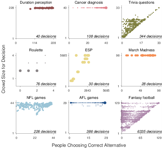
| Figure 1: Summary of observed behavior in nine data sets. In each panel, the y-axis corresponds to the number of individuals in the crowd making a decision, and the x-axis corresponds to the number of individuals choosing the correct alternative for that decision. The area of the circles corresponds to the number of decisions in the data set with each count of individuals being correct and crowd size. The total number of decisions in the domain is also listed. |
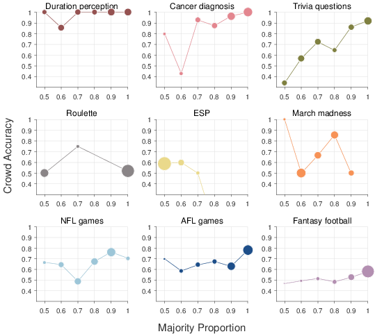
| Figure 2: Calibration curves relating the majority size to its average accuracy. Each panel corresponds to a data set. The x-axis corresponds to the proportion of individuals who chose the majority alternative, grouped into bins. The y-axis corresponds to the proportion of decisions in each bin for which the majority was correct. The area of each circle is proportional to how many decisions belong to each majority-size bin. |
2.1 Duration perception
The data come from two psychophysical discrimination tasks, involving visual and auditory duration perception, reported by van Driel et al. (2014). In the auditory task, individual participants judged the duration of auditory beeps, while in the the visual task they judged the duration of an LED light. In both tasks, a trial consisted of a 500 ms standard, followed by a 1000 ms inter-stimulus interval, and then a target stimulus of variable duration. Each participant on each trial indicated whether they perceived the target stimulus to be longer or shorter than the standard. A total of 19 participants completed 3 blocks of 80 trials for both the auditory and visual tasks, in a within-subjects design.
The same 20 unique target durations were used in both conditions. We treat each unique duration for each modality as a decision, giving a total of 40 decisions for the data set. We collected all of the responses made by any participant to that target duration in that modality. For example, the target stimulus with duration 470 milliseconds in the visual condition was judged to be shorter than the standard on 146 of the 227 trials on which it was presented. Thus, for this decision, the majority is about 64%, and is correct. In the “duration perception” panel of Figure 1, this decision is shown at an x-value of 146, and a y-value of 228, because 146 correct decisions were made for the stimulus, out of a total of 228 presentations. In the “duration perception” panel of Figure 2, this decision contributes to the point at an x-value of 0.6 because its majority falls in the bin between 0.55 and 0.65. The corresponding y-value of 0.86 arises because 6 out of the 7 duration decisions with majority sizes falling in this bin were correct.
Overall, the “duration perception” panel of Figure 1 shows that most of the decisions are based on crowd sizes near the maximum of 228, and that the majority of individuals generally choose the correct alternative. The corresponding calibration curve in Figure 2 shows that the majority decision is almost always correct, even for decisions in which the majority is made up of only slightly more than half of the individual judgments.
2.2 Cancer diagnosis
The data come from Argenziano et al. (2003), and involve cancer diagnoses made by each
of 40 dermatologists for the same 108 skin lesions. The dermascopic
images were presented online, and a two-step diagnostic procedure was
used, first distinguishing melanocytic from non-melanocytic lesions,
and then distinguishing melanoma from benign lesions. The second step
incorporated standard diagnostic algorithms as decision-making aids.
We treat each lesion as a decision. The “cancer diagnosis” panel in Figure 1 shows that majority of dermatologists chose the correct diagnosis for most lesions, and often there is strong agreement between the dermatologistis. The corresponding calibration curve in Figure 2 shows an increase in accuracy with an increasing majority, and that decisions are almost always correct when there is near-complete agreement.
2.3 Trivia questions
The data come from research reported by Bennett, Benjamin and Steyvers (2018), and involve individual participants answering trivia questions. We consider data from multiple experimental conditions involving the same set of 144 questions, 24 of which are “catch” questions with obvious answers. The conditions vary in terms of whether or not individuals can choose which questions they answer, along the lines described by Bennett, Benjamin and Steyvers (2018).
We treat every question in every experimental condition as a decision. The “trivia questions” panel in Figure 1 shows that anywhere between a single individual and 33 individuals were involved in the various decisions, with most decisions involving fewer than 20 individuals. It is clear there are some questions for which most individuals gave the correct answer, but also many decisions with many incorrect answers. The corresponding calibration curve in Figure 2 shows an increase in accuracy with an increasing majority, qualitatively much like the cancer diagnosis curve, with the possible difference that decisions based on very small majorities seem to be accurate less than half the time.
2.4 Roulette
The data come from Croson and Sundali (2005), and involve people’s gambling decisions playing the standard casino game of roulette. The data were manually extracted from 18 hours of hotel security footage recorded over a 3-day period from a Nevada casino in 1998. We considered only the gambles in which a player placed chips on the (near) binary possibilities “red” vs. “black” or “odd” vs. “even”, and counted multiple chips placed by the same player as a single choice.
We treat each spin of the roulette wheel for which there was more than one bet as a decision. The “roulette” panel in Figure 1 shows that the 76 decisions involved at most four players, and the vast majority only involved two players. The number of individuals making correct decisions seems uniformly distributed for each crowd size. The corresponding calibration curve in Figure 2 shows that accuracy is always consistent with chance, whether the majority is only half the crowd or the majority is the entire crowd.
2.5 Extrasensory perception
The data come from the analysis of the Zenith radio experiments undertaken by Goodfellow (1938). These experiments in telepathy in the 1930s involved a radio program “transmitting” binary signals, by informing their listening audience that a group of telepathic senders in the studio was concentrating on one of two possible symbols, such as a circle or a square. The audience was asked to determine which symbol was being transmitted, and invited to mail responses indicating the signals they believed were sent, for a set of transmissions conducted over the course of the program. We consider the specific results in Goodfellow (1938), Table II, which detail the frequency of responses to all 32 possible sequences of 5 binary signals, for 6 different stimulus types, as well as listing the true signal. Using the total number of respondents for each stimulus type, we converted these frequencies to counts for each individual signal. The counts are approximate, given the limited precision of the provided frequencies.
We treat each signal for each stimulus type as a decision. The “ESP” panel in Figure 1 shows that, for most of the decisions, about half the respondents chose the correct answer. It is also that the decisions span a wide range of crowd sizes, ranging from about 1000 individuals to just under 6000 individuals. The corresponding calibration curve in Figure 2 reinforces that the majorities are generally near half the crowd, but shows a proportion of accurate decisions around 60%.
2.6 March madness
The data come from Carr and Lee (2016), and involve participants predicting which of two basketball teams would win a game in the 2016 “March madness” U.S. collegiate tournament. The same 98 participants predicted the winner of the 28 first-round games not involving wild-card teams. The predictions were made online, as part of an Amazon Mechanical Turk study, in which participants completed a simple survey asking them to predict the winner of each game, and indicate whether or not they recognized each team. No information about the teams — such as tournament seedings, betting market probabilities, or expert opinions — were provided, although there was nothing preventing participants obtaining this information in making their predictions.
We treat each game as a decision. The “March madness” panel in Figure 1 shows a wide range of agreement and accuracy over the decisions. The corresponding calibration curve in Figure 2 is noisy, because of the relatively small number of decisions, but generally suggests an increase in accuracy with an increasing majority.
2.7 NFL games
The data come from Simmons et al. (2011), who recruited American football fans from the general public, and collected various predictions about the 2006 NFL season from them through an online competition. We use predictions only from the “estimate” group of 45 fans, who predicted the outcome of 226 Sunday games. Other groups in the Simmons et al. (2011) made predictions relative to a betting measure known as the point spread, rather than directly predicting the winner of each game.
We treat each game as a decision. The “NFL games” panel in Figure 1 shows that the number of correct decisions ranges from none of the fans to all of them. It also shows that not every fan made a prediction about every game, leading to variability in the crowd size over decisions. The corresponding calibration curve in Figure 2 shows that, in general, as the majority increases in size, the crowd decisions tend to become more accurate. Even when there is complete consensus, however, only about 70% of games are correctly predicted. It is also clear that many decisions involve large majorities.
2.8 AFL games
The data come from pundit predictions for the 198 games played in the
regular season of the Australian Football League in 2015 and
2016.1 The predictions were made by a regular
set of 29 pundits, most of whom made predictions about every game, in
a weekly column in the Melbourne Herald Sun newspaper, published online at heraldsun.com.au. Some pundits were AFL expert commentators or former players, and some were politicians or prominent athletes from other sports.
We treat each game as a decision. The “AFL games” panel in Figure 1 shows that the number of correct decisions ranges, as for the NFL data set, from none of the pundits to all of them. There are more decisions for which there is unanimous agreement than for the NFL games data set. The calibration curve for the AFL games in Figure 2 shows, with considerable noise, an increase in accuracy with increasing majority.
2.9 Fantasy football
The data come from the website fantasypros.com, which collates expert opinion on which of two players will perform best in an American fantasy football competition each week.2 The comparisons are presented for each of the standard fantasy football positions, and generally include all possible combinations of players likely to be available in a typical fantasy league. We collected the data from week 8 to week 17 inclusive of the 2015–2016 season, at various non-systematic times between the end of the Monday night game for one week and the beginning of the Thursday night game for the next week. Depending on the timing, and depending on the players being compared — since some experts make predictions for more limited sets of players than others, and post their predictions at different times between Monday night and Thursday morning — the crowd size varies from 6 to 129. As a concrete example, the first player combination collected in week 8 was the quarterback comparison of Tom Brady and Phillip Rivers by 127 experts, 88 of whom recommended Brady. These experts turned out to be correct, since Brady scored about 34 points, while Rivers scored about 27, using standard scoring data we collected from the website fftoday.com.
We treat only a subset of all the available comparisons as decisions, with the intent of considering only those comparisons that would realistically be encountered in playing fantasy football. Specifically, we considered only comparisons in which both players had an average fantasy football score over the weeks considered that exceeded a threshold for their position — 10 points for quarterbacks, running backs, and wide receivers, and 5 points for tight ends, kickers, and defense and special teams — and the difference in the means between the two players was less than 5. These restrictions are an attempt to identify players that are likely owned in fantasy football leagues, and comparisons between players that are close enough that expert advice might be sought. Overall, the restrictions resulted in a total of 6335 player comparisons being treated as decisions.
The “fantasy football” panel in Figure 1 shows a wide range of crowd sizes, and it seems that often nearly every expert is either correct, or nearly no expert is correct. This pattern is made clear in the calibration curve in Figure 2, which shows a large majority for most decisions. The calibration curve also shows, however, that even these highly-agreed decisions are correct only about 60% of the time, and decisions with majorities proportions below about 0.8 are correct no more often than chance.
3 Discussion of Empirical Results
The empirical results show that the relationship between the size of the majority and crowd size can take many forms. A reasonable prior expectation about the relationship might resemble the cancer diagnosis calibration curve in Figure 2, in which progressively larger majorities lead to progressively greater accuracy. The other calibration curves in Figure 2, however, show a set of other possibilities. These variations seem theoretically and practically interpretable and important.
The duration perception domain suggests that it is possible for even very small majorities to be very accurate. The calibration curve shows that even if a tone duration is judged to be longer than the standard only slightly more often than it is judged to be shorter, it is almost certainly the case it was really longer. One interpretation is that the simple psychophysical judgments being made are completely independent of each other, even in those cases where it is the same participant making a judgment about the same target duration on a different trial. Given some objectively correct signal, completely statistically independent noise, and a reasonable crowd size, it is theoretically reasonable to expect high accuracy even for small majorities.
The trivia questions domain suggests that it is possible for majorities to be incorrect systematically. The calibration curve shows that narrow majorities are correct less than half the time. One interpretation is that this happens because of trick questions, designed to prompt answers driven by widely-held beliefs that are factually incorrect.
Both the roulette and ESP domains suggest that it is possible for accuracy to be independent of majority size. The calibration curves show accuracy near chance, independent of the size of majorities for various decisions. The obvious interpretation is that this is because these domains do not involve signals that provide any useful information. Even if everybody puts their money on black in roulette, they are right only (about) half the time.
Finally, all of the March madness, NFL games, AFL games, and fantasy football prediction domains suggest that it is possible for there to be an upper limit on crowd accuracy. All of the calibration curves show accuracy well below 100% even when decisions are near unanimous. In contrast, the duration perception, cancer diagnosis, and trivia question calibration curves show near-perfect accuracy when decisions are near unanimous.
Collectively, these findings suggest that the relationship between majority size and accuracy, and the distribution of majority sizes over decisions in a domain, are variable and complicated. Calibration curves do not always progress from the bottom-left (small majority, low accuracy) to the top-right (large majority, high accuracy). They can pass through the top-left (small majorities, high accuracy), the bottom-right (large majority, low accuracy), and anywhere in between.
The other information summarized in Figure 2 relates to the distribution of majority sizes over all the decisions in a domain. This is shown by the area of the circles for each majority-size bin. It is less clear what a reasonable prior expectation about this distribution might be. For decisions that individuals as well as groups can make accurately, large majorities should be observed. Even for inaccurate decisions, the concept of “group-think” — which emphasizes the possibility people in groups chose in a way that avoids creative or independent thinking, and attempts to avoid individual responsibility for group decisions — suggests it is possible for most individuals to favor one alternative, if individuals are aware of the choices of others. For example, (Surowiecki, 2004, p. 47) discusses the concept of risk-averse “herding” as possibly accounting for most American football coaching groups not attempting many fourth downs, despite some evidence it would be better to do so.
The nine data sets show a range of results in terms of the distribution of majority size. Both the fantasy football and AFL games domains do show many decisions with large inaccurate majorities, consistent with herding. The other NFL games and March madness domains show a broader distribution of majority sizes. The cancer diagnosis domain also shows many large majorities, presumably because of individual expertise. The duration perception and trivia questions results show a broad range of majority sizes. The roulette domain is based on very small crowd sizes, while the ESP domain is based on very large crowd sizes that are almost always evenly divided.
Thus, it appears that, just as for the relationship between majority size and accuracy, there are few general regularities in the distribution of majorities. It is also clear that the distribution of majorities is not closely tied to overall accuracy. The fantasy football results make it clear that most decisions having large majority does not indicate high accuracy, and the duration perception results make it clear that high accuracy can be achieved without most decisions having large majorities.
4 A Logistic Growth Model of Majority and Accuracy
The calibration curves in Figure 2 provide evidence
that the relationship between majority size and crowd accuracy can
take a number of forms. Drawing strong conclusions based on this sort
of empirical analysis, however, is difficult. The binning assumptions
used to generate the curves in Figure 2 are not
principled, and different choices of bin widths lead to
quantitatively, if not qualitatively, different curves. It is clear
that calibration curves for most of the data sets are noisy, and it is
impossible to determine what variation is signal and what variation is
noise by the visual inspection of Figure 2.
The potential problems associated with making inferences by the visual inspection of calibration curves based on arbitrary binning assumptions, are highlighted by an animation, available at https://osf.io/v9zcr/, that shows how the curves change as the bin width is changed.
Part of the problem is that simple empirical analysis largely ignores the underlying uncertainty inherent in inferring the majority size and crowd accuracy from the behavioral data. A majority of 1 out of 2 people in the roulette data set is treated as equally good evidence for a 0.5 majority as 2500 out of 5000 people in the ESP data set. Similarly, the uncertainty inherent in inferring the crowd accuracy from binary outcomes is based on simple proportions of the binned decisions, and there is no attempt to quantify uncertainty. This makes it difficult, for example, to draw conclusions about whether majorities around 0.5 in the trivia questions data set really perform worse than chance, or whether the drop in accuracy for majorities of 0.6 for the duration perception data set is somehow “significant”.
Even more importantly, the failure to incorporate uncertainty in the empirical analysis makes it impossible to make principled inferences about the underlying form of the calibration function. For example, the accuracy of the crowd appears to increase with increasing majority sizes for both the NFL games and AFL games data sets, but it is not inconceivable they are constant, and the observed fluctuations are due to sampling variability. If they do increase, it is certainly not obvious whether they do so at the same rate. Nor is it obvious whether one game is inherently more unpredictable than the other, in the sense that a unanimous crowd is more accurate in one case than the other.
To address these sorts of questions requires modeling the data, by making assumptions about the underlying form of the calibration function relating majority size and crowd accuracy. Inferences about the underlying calibration function, and about meaningful parameters of that function — such as the rate of increase in accuracy with majority, or the ceiling level of accuracy achieved by unanimous crowds — can then be made by applying the model to the behavioral data. Accordingly, in this section we develop a modeling approach, based on standard statistical logistic-growth models.
4.1 A general logistic-growth model
Each of the nine data sets can be formally described as follows: there are n decisions, and the ith decision has ki people making the majority decision out of a crowd of ni people, with an accuracy of yi=1 if the majority decision is correct, and yi=0 otherwise. For each decision, the key latent variables of interest are the proportion θi representing the size of the majority, and the probability φi representing the probability the majority of the crowd is correct.
We make the obvious assumptions that the observed majority size follows a binomial distribution with respect to the underlying majority proportion and the crowd size
| ki ∼ Binomial | ⎛
⎝ | θi,ni | ⎞
⎠ | ,
|
and the observed crowd accuracy is a Bernoulli draw with respect to the underlying accuracy
We also model the distribution of majority proportions across all of the decisions as coming from an over-arching truncated Gaussian distribution, so that
| θi ∼ Gaussian | | ⎛
⎝ | µ,1/σ2 | ⎞
⎠ | ,
|
where µ∼Uniform(1/2,1) and σ∼Uniform(0,1/2) are the mean and standard deviation, respectively.
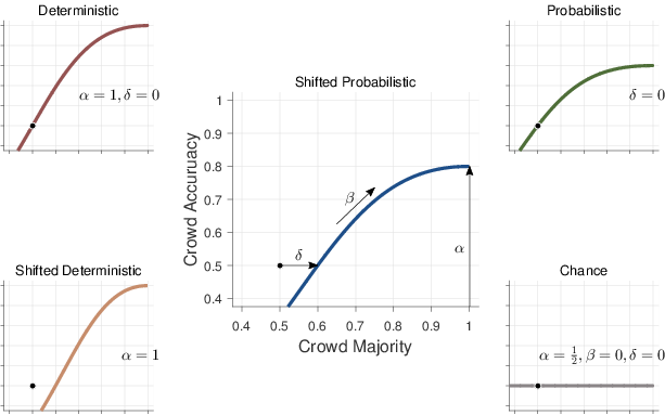
Understanding the relationship between majority size and accuracy involves formalizing a calibration function that determines the accuracy for each possible given majority, φi = fψ(θi ), where ψ are parameters of the calibration function. We focus on one candidate calibration function, based on the standard Verhulst logistic growth model widely used throughout the empirical sciences (Weisstein, 2017). This model is typically applied to phenomena — such as population growth, biological growth, the spread of language, the diffusion of innovation, and so on — in which growth is bounded. It seems well suited to the current problem because of logically bounded nature of crowd accuracy.
| Figure 3: Empirical calibration curves relation the proportion of decision makers in the majority on the x-axis, to the average accuracy of the majority decision on the y-axis. |
Formally, we consider what we term a shifted probabilistic logistic growth model
| φi = | | α |
|
| 1+exp | ⎧
⎨
⎩ | −β [log | | −log | | − | | ] | ⎫
⎬
⎭ |
|
| ,
(1) |
with a growth parameter β, a bound parameter α, and a shift parameter δ. This model is shown in the central panel of Figure 3. The upper bound on accuracy is controlled by α. As the size of the majority increases, the accuracy of the crowd increases at a rate controlled by β, with β=1 corresponding to a linear increase, values β>1 corresponding to faster increases, and values β<1 corresponding to slower increases. In the limit β=0, there is no growth in accuracy, and it is constant for all majority sizes. The shift of the growth curve is controlled by δ. When δ=0 a majority of one-half (i.e., the crowd is evenly divided between both alternatives) has chance accuracy. When δ>0 the curve is shifted to the right, as shown, meaning that majorities greater than one-half can perform at chance, and small majorities can perform worse than chance.
The parameterization of the shifted probabilistic model given by Equation 1 is intended to help the meaningful interpretation of the parameters, and hence help in setting priors.3 For the upper bound on accuracy, we use
corresponding to the assumption that best possible accuracy in a domain is equally likely to be anywhere from chance to perfect accuracy. For the growth of accuracy. we use
which has its mode at β=1, corresponding to the assumption that
the most likely growth rate is linear, but allows for any growth rate
β>0. The exact form of the prior was chosen by examining the
implied prior over calibration functions, using the approach advocated
by Lee and Vanpaemel (2018), and demonstrated by
Lee (2018). For the shift in the calibration curve, we use
This prior makes the assumption that if the calibration curve is shifted, it can only be shifted to the right, and that all rightward shifts are equally likely. These shifts have the effect of decreasing the accuracy of majorities, consistent with the possibility that no signal is accumulated until some significant majority is achieved. Leftward shifts, in contrast, have the effect of increasing the accuracy of majorities. These increases, however, are what the growth parameter β is intended to capture. Thus, for model identifiability and interpretation, only rightward shifts are incorporated in the model.
4.2 Special case models
We also consider four special cases of the full shifted probabilistic model, shown in the surrounding panels of Figure 3. The deterministic model in the top-left corresponds to setting δ=0, α=1, and allowing only β to vary. This model thus assumes that perfect accuracy is achieved for large majorities, and that one-half majorities perform with chance accuracy. This special case of the general model is expected to be appropriate for book knowledge, or other domains in which the ground truth exists, and a reasonable number of people in the crowd might know the correct answer. In this case, it is reasonable to expect a large majority to correspond to a correct answer, and an evenly-divided crowd to correspond to a guess. The free parameter β corresponds to how quickly an increasing majority moves from guessing to correct decisions.
The shifted deterministic model in the bottom-left corresponds to setting just α=1, allowing for worse-than-chance performance. This special case is expected to be appropriate where a domain includes decisions that are actively misleading, or for which people systematically produce incorrect answers. There is evidence that this can happen in the related literature on the calibration of individual probability estimates. Lichtenstein and Fischhoff (1977), Figure 6, for example, observe worse-than-chance performance in a calibration analysis considering the worst participants answering the most difficult questions in a general knowledge task similar to our trivia question domains. In these cases, the free parameter δ corresponds to the increase over one-half needed for a majority to reach chance accuracy.
The probabilistic model in the top-right corresponds to setting just δ=0, and allowing only β to vary. This model assumes one-half majorities perform with chance accuracy, and accuracy grows to some upper bound α as majorities increase. Conceptually, this bound applies when the crowd fundamentally lacks the ability to make completely accurate decisions. Potentially, this could occur if a ground truth exists, but the information needed to determine this truth is not available to the crowd. Perhaps more interestingly, this situation will arise when the ground truth itself is yet to be determined, and is subject to future events that cannot be known with certainty, as is the case when the crowd is making predictions. In these cases, the free parameter α corresponds to the upper bound measuring the inherent (un)predictability of the domain, and β corresponds to how quickly that limit is approached.
Finally, the chance model in the bottom-right corresponds to setting α=1/2, β=0, and δ=0, which reduces the full shifted probabilistic model to θ=1/2 for all majority sizes, so that accuracy is always at chance. This special case is expected to be appropriate in domains where little or no signal is available, and crowds cannot make effective decisions. Again, there is evidence in the individual probability calibration literature that this can be empirically observed (e.g., Lichtenstein and Fischhoff, 1977, Figure 2).
4.3 Latent-mixture implementation
We implement the model as a graphical model in JAGS (Plummer, 2003), which allows for fully Bayesian inference using computational sampling methods. We treat the full shifted probabilistic model, and its four special cases, as components of in a latent-mixture model. The assumption is that all of the decisions in a domain follow one of these five calibration curves, so that
|
| | φi | = | ⎧
⎪
⎪
⎪
⎪
⎪
⎪
⎪
⎪
⎪
⎪
⎪
⎪
⎪
⎪
⎪
⎪
⎪
⎪
⎪
⎪
⎪
⎨
⎪
⎪
⎪
⎪
⎪
⎪
⎪
⎪
⎪
⎪
⎪
⎪
⎪
⎪
⎪
⎪
⎪
⎪
⎪
⎪
⎪
⎩ | | if z = 1
|
| 1/ | ⎛
⎝ | 1+exp | ⎧
⎨
⎩ | −β | ⎡
⎣ | log | | ⎤
⎦ | ⎫
⎬
⎭ | ⎞
⎠ |
| if z = 2
|
| |
| if z = 3
|
| |
| − | | log | ⎛
⎝ | 2α−1 | ⎞
⎠ | ⎤
⎦ | ⎫
⎬
⎭ | ⎞
⎠ |
| if z = 4
|
| |
| |
| − | | log | ⎛
⎝ | 2α−1 | ⎞
⎠ | ⎤
⎦ | ⎫
⎬
⎭ | ⎞
⎠ |
| if z = 5
|
| |
| |
| | | | (-2) |
|
with each mixture component given equal prior probability
The JAGS script is provided in the supplementary material. We applied this model to each of the nine data sets, collecting 1000 samples from each of 4 independent chains, thinning by retaining every 10th sample, after discarding 1000 burn-in samples from each chain. Convergence was checked by visual inspection, and using the standard R-hat statistic (Brooks and Gelman, 1997).
5 Discussion of Modeling Results
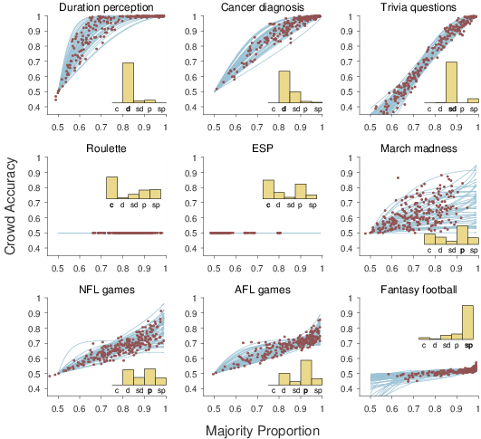
| Figure 4: Results from applying the latent-mixture logistic growth model to the nine data sets. Each panel corresponds to a data set. The inset histogram shows the posterior probability of the 5 mixture component models (“c” = chance, “d” = deterministic, “sd” = shifted deterministic, “p” = probabilistic, “sp” = shifted probabilistic). The most likely model is labeled in bold. The lines show samples from the posterior distribution of the most likely calibration model, and the circular markers show samples from the joint distribution of majority proportion θ and crowd accuracy φ aggregated over all of the decisions. |
Figure 4 and Table 1 summarize the results of applying the latent-mixture logistic-growth model to the nine data sets. The inset histogram shows the posterior probability of the five possible models, ranging from the simplest chance model to the shifted probabilistic model. These probabilities quantify how likely each model is, based on the decision data, taking account of both goodness-of-fit and the complexity of each model. The lines in Figure 4 show samples from the posterior distribution of the inferred calibration curve. These samples are based on the joint posterior parameter distribution for the model with the greatest posterior probability.4 Also shown by circles are samples from the joint posterior distribution of the majority proportion θ and crowd accuracy φ aggregated over all of the decisions.
Accompanying the results in Figure 4, Table 1 lists the most likely model for each data set, and the marginal posterior expectation of the relevant parameters. Every model includes the mean µ and standard deviation σ over the majority proportions. Depending on the inferred model, the growth β, upper bound α, and shift δ are also detailed.
| Table 1: Model and parameter inferences applying the latent-mixture logistic-growth model to the nine data sets (“det” = deterministic, “shift det” = shifted deterministic, “prob” = probabilistic, “shift prob” = shifted probabilistic). |
| | | | Majority | | Accuracy |
|
Data set | Model | | µ | σ | | β | α | δ |
| Duration perception | det | | 0.93 | 0.24 | | 3.82 | – | – |
| Cancer diagnosis | det | | 0.98 | 0.18 | | 1.68 | – | – |
| Trivia questions | shift det | | 0.78 | 0.17 | | 1.57 | – | 0.14 |
| Roulette | chance | | 0.85 | 0.07 | | – | – | – |
| ESP | chance | | 0.54 | 0.07 | | – | – | – |
| March madness | prob | | 0.72 | 0.12 | | 1.82 | 0.73 | – |
| NFL games | prob | | 0.83 | 0.15 | | 0.99 | 0.82 | – |
| AFL games | prob | | 0.99 | 0.17 | | 1.32 | 0.78 | – |
| Fantasy football | shift prob | | 1.00 | 0.13 | | 0.77 | 0.59 | 0.29 |
The duration perception and cancer diagnosis domains are inferred to have deterministic calibration curves. This makes sense, since it corresponds to there being a ground truth, and perfect accuracy being achievable. The inferred growth parameters indicate that crowd accuracy increases very quickly for duration perception, and moderately quickly for cancer diagnosis. The inferred majority proportion parameters show that, on average, majorities are large, but there is considerable variation across decisions. This is especially true for duration perception.
The trivia questions domain is inferred to have a shifted deterministic calibration curve. The natural interpretation comes in two parts. The first part, corresponding to the deterministic model inference, is that there are ground truth answers, so that perfect accuracy is achievable. The inferred growth parameter shows that accuracy improves as majority increases at about the same rate for the cancer diagnosis domain. The second part, corresponding to the shifted model inference, is that some of the trivia questions are “trick” or misleading questions, for which small majorities have worse than chance accuracy. The inferred shift parameter shows that about a 65% majority is needed to reach chance accuracy, and an evenly-divided crowd is correct less than 40% of the time. The inferred majority proportion parameters show that about 75% of the crowd agrees on average, but there is again significant variability in this proportion across decisions.
Both the ESP and roulette domains are inferred to follow the chance model. For the roulette data set, this finding is easily interpreted, and is not surprising. The domains was chosen because of the expectation that there is no objective accuracy signal, and no wisdom of the crowd effect is possible. No matter how many people bet on red, they are right — approximately, allowing for the lone green outcome — half of the time. The interpretation of the specific ESP data set we used is more subtle. The emphasis of the Goodfellow (1938) analysis is on the non-uniform choices people make when generating “random” sequences, and the subtle influence of stimuli and instructions, as possible accounts of better-than-chance performance in the ESP task. The need for such an account is evident in the above-chance accuracy in the empirical calibration curve in Figure 2. The inference of the chance calibration curve presumably results, in part, from the absence of evidence of an increase in accuracy with increasing majorities, as predicted by the other calibration curve models. It is worth noting that Figure 4 shows that some significant posterior probability was inferred for the probabilistic model, consistent with a tension between these two possibilities in the data.
The March madness, NFL games, and AFL games domain are all inferred to have a probabilistic calibration curve. This makes sense, since all three involve predictions, and there is irreducible uncertainty in the outcome. The inferred upper bound parameter provides an estimate of the level of irreducible uncertainty, finding best-case predictabilities of 73%, 82%, and 78%, respectively, for the three domains. The inferred growth parameter show that March madness predictions become accurate more quickly as the majority increases, followed by AFL games, and then NFL games. The inferred majority proportion parameters show an interesting disconnect between the typical sizes of majorities, and these inferences about the growth and upper bound on crowd accuracy. In particular, the AFL games data set shows much greater mean majority proportions, despite have a moderate growth and upper bound compared to the March madness and NFL games data sets. This is compatible with some form of “herding” for the AFL games experts, in the sense that they all tend to make the same predictions, without any justification in terms of crowd accuracy.
Finally, the fantasy football domain is inferred to have a shifted probabilistic calibration curve. The probabilistic part of the inference makes sense for the same reasons as the March madness, NFL games, and AFL games domains. Predicting which fantasy football player to start involves irreducible uncertainty. The inferred upper bound parameter shows that there is a very low ceiling of 59% accuracy. The inferred shift parameter shows the crowd reaches better-than-chance performance only once there is a majority proportion of about 80%. The inferred growth parameter connects these two findings, showing a slow increase in accuracy with increasing majorities. The inferred majority proportion parameters show a remarkable disconnect with the low accuracy. The average majority proportion is effectively unanimity, and there is only moderate variability. This is compatible with significant herding, in which most experts chose the same player for most decisions, despite the low accuracy of these predictions.
6 General Discussion
The core of the wisdom of the crowd phenomenon is the possibility of generating good group judgments from individual judgments. Any application of the crowd judgment, however, benefits from knowing how accurate it might be. The decisions made by individuals are more useful if we know much confidence can be placed in them. The same is true of crowd decision. Other than examining the calibration of prediction markets, and some work in forecasting, however, there appears to be little research evaluating the confidence that should be placed in crowd judgments. More fundamentally, there appear to be few methods for making predictions about the accuracy of crowd judgments in the first place.
In this paper, we have taken first steps towards understanding the confidence that can be placed in crowd judgments, for the simple but fundamental case in which individuals choose between two discrete alternatives. For binary judgments, an obvious measure of the confidence of a crowd is the size of the majority. Thus, our primary research questions was to understand the relationship between majority size and accuracy. A secondary question was to understand the distribution of majority sizes over decisions, especially as this distribution might relate to overall accuracy.
Using nine diverse data sets, we found evidence that neither question has a simple answer. In terms of the calibration curve relating majority size to accuracy, we found domains in which increasing majorities tend to be more accurate, but also domains in which small majorities were just as accurate, and domains in which larger majorities were not more accurate. In terms of the distribution of majority sizes, we found domains in which there was a broad distribution over decisions, and other domains in which most decisions had large majorities. Sometimes, however, these large majority domains involved very accurate crowd judgments, and sometimes they involved very inaccurate crowd judgments.
Given this empirical diversity, an important first step to understanding is to be able to measure the features of a domain. Accordingly, we developed a measurement method, based on logistic growth models. We applied this model to the nine data sets, using Bayesian analyses that acknowledge the uncertainty in the behavioral data, and allow for inferences about psychological meaningful models and parameters. In particular, the measurement model contains interpretable components corresponding to how quickly accuracy grows as the majority increases, whether or not a domain has irreducible uncertainty, and whether majorities can be systematically wrong.
The measurement method was shown to make sensible inferences for nine data sets, and these results demonstrate the potential for its application. Most obviously, the inferred calibration curves allow the probability of the accuracy of a crowd judgment to be estimated from the size of the majority on which it is based. From the results in Figure 4, if 70% of the individuals in a crowd judges a duration to be longer than a standard, it almost certainly is, if 80% of dermatologists judge a skin lesion to be cancerous, there is a 70–95% probability that it is, and if 90% of a trivia team agree on a true-false answer, there is about a 90% probability they are right. More surprisingly, the same trivia questions calibration curve suggests that if below 65% of the team agrees, it is probably a trick question, and it would be better to choose the minority decision. The calibration curves for the prediction domains are obviously extremely useful for betting, where decisions needs to be made in the context of specific monetary payoffs. For example, if more than 80% of pundits agree on an AFL game winner, there is at least a 60% probability they are right, and odds better than this are worth taking.
Our modeling approach has interesting applications beyond inferring the calibration curve, coming from the latent mixture approach. The four data sets involving predictions about uncertain future events were correctly inferred, and led to an inference about the upper bound on achievable accuracy. These bounds are relevant to the general question of distinguishing between games of chance, such as roullette, or games of skill, such as chess. One way to conceive of the distinction is that games of skill have some minimum level of predictability, and the α parameter is one way to operationalize this level for a given domain. This is important for public policy debates, especially in legal jurisdictions where games of chance are illegal, but games of skill are not. As a recent concrete example, the legality of a daily fantasy sports is debated in terms of this distinction, with public, political, and legal opinion divided (Meehan, 2015). Our results reflect on this debate, since the upper bound for fantasy football was inferred to be around 60%, between the 50% of roulette and the approximately 80% of NFL and AFL games. Setting a threshold on α delineating chance from skill would be one way to codify public policy.
Other applications to policy are suggested by the jurisprudence and economic governance examples we mentioned in the introduction as motivations for studying the calibration of binary choice. For example, different American states sometimes allow collective jury decisions to be based on less-than-unanimous individual juror decisions (Suzuki, 2015). Inferred calibration curves relating the size of the majority in a jury to the accuracy of that decision — presumably measured at some later date based on additional evidence — would allow an appropriate threshold of agreement to be determined for a desired level of accuracy. An advantage of the model-based approach adopted here is that such an analysis would incorporate uncertainty in a principled way. It would also allow for extrapolation and interpolations to situations not observed in empirical data. For example, the β parameter can be interpreted as the rate of increase in accuracy with additional juror agreement, which would allow inferences to be made about the accuracy of jury sizes and majorities not currently used in practice. Similarly, the level of agreement needed among voting members of the Federal Reserve Board when a decision is made to raise or lower interest rates could be studied in terms of its calibration with subsequent economic success or failure.
An advantage of taking a modeling approach, and our use of fully Bayesian methods for statistical inference in applying models to data, is that uncertainty is represented and incorporated into analyses. This advantage applies to issues involving both model selection and parameter estimation (Wagenmakers, Morey and Lee, 2016). Identifying the appropriate calibration curve is effectively a model selection problem, and our approach automatically balances goodness-of-fit and complexity in making these inferences. The answers to practical questions based on calibration curve parameters will similarly benefit from knowledge of the uncertainty in their estimation. For example, asking whether the NFL or AFL is more inherently predictable amounts to determining the probability that the upper bound α is greater for the NFL, which can be done by comparing their posterior distributions. Similarly, it would be possible to determine whether accuracy grows more quickly with increasing expert consensus in the NFL than the AFL by comparing the posterior distributions of their β growth rate parameters. The answers to these questions will themselves be uncertain, giving the probability the NFL exceeds the AFL, reflecting the fundamental uncertainty in inference from limited data.
Looking ahead, our modeling approach also sharpens the theoretical challenges involved in understanding the wisdom of the crowd for binary decisions. The variety of calibration curves observed empirically in Figure 2 ultimately needs to be explained in terms of the psychology of individual decisions. While the measurement model provides a useful way to characterize the relationship between majority size and accuracy, it does not provide an account at the level of the basic underlying psychological processes. Existing theoretical frameworks for the wisdom of the crowd (Davis-Stober et al., 2015; Grofman, Owen and Feld, 1983) typically make strong assumptions that provide analytical tractability, but will almost certainly need to be relaxed to explain the sorts of calibration curves we observed.
At least three components seem important for a successful psychological model. One required component is an account of the environment, allowing for both knowable ground truths and irreducible uncertainty, and allowing for domains where accuracy signal range from very strong to non-existent. The nature of the environment also needs to be incorporated: most of our data sets involved “neutral” environments passively providing information, but the ESP environment was helpful in the way the pseudo-random signals were generated, and the trivia question environment was adversarial in its use of trick questions. A second required component is an account of the cognitive processes that convert the knowledge of individuals to their judgments. This involves assumptions about both expertise, and the basic decision-making processes that produce the behavioral judgment. It also involves understanding the goals and incentives involved in making decisions: the goal in duration perception is simply to be accurate, but there may be an incentive to pick unlikely winners (“dark horses”) in sports predictions. The third required component is an account of the social influences individuals have on each other. In some of our data sets, individuals made decisions independent of each other, but in others some individuals could see the decisions of others. Thus, assumptions need to be made about how this visibility affects individuals, including possibilities like herding. Even in situations where individuals make judgments independently, it is likely they are sensitive to the possible opinions of others, especially in competitive settings (Lee, Zhang and Shi, 2011; Prelec, Seung and McCoy, 2017). Thus, a complete psychological model needs to incorporate environmental, cognitive, and social theories, to explain when and why calibration curves take different forms. We think the development of a psychological model, to complement the measurement model developed here, should be a priority for future research.
Finally, it would be possible to extend the study crowd calibration beyond the simple binary decision-making case considered here. One way to think of the calibration curve is that it relates a measure of the confidence a crowd has in its decision to the eventual accuracy of that decision. In the binary case, it is natural to measure confidence in terms of the size of the majority. This measure could be equally well applied to multiple-choice decisions, and so our model generalizes immediately to discrete choices with more than two alternatives. For continuous choices, such as scalar estimation, different measures of the confidence a crowd has in its decision need to be defined. In some cases, such as prediction markets, this seems straightforward. The complicated aggregation mechanism used by prediction markets generates a crowd probability that can be compared to accuracy, leading to the sort of calibration curve analyses presented by Page and Clemen (2012). For other scalar estimation situations, such as the basic wisdom of the crowd problem of estimating the number of jelly beans in a jar, additional assumptions need to be made. One possibility is that some measure of the dispersion of individual estimates — such as the variance, or the range — is a useful indicator of crowd confidence (Kurvers et al., 2016). How these sorts of measures of the confidence of crowd estimates relate to the accuracy of those estimates is an interesting and important generalization of the calibration surves for binary decisions we have considered.
-
-
Argenziano, G., Soyer, H. P., Chimenti, S., Talamini, R., Corona, R., Sera, F.,
Binder, M., Cerroni, L., De Rosa, G., Ferrara, G., et al. (2003).
Dermoscopy of pigmented skin lesions: Results of a consensus
meeting via the internet.
Journal of the American Academy of Dermatology, 48:679--693.
[ bib ]
-
-
Bahrami, B. and Frith, C. D. (2011).
Interacting minds: a framework for combining process-and
accuracy-oriented social cognitive research.
Psychological Inquiry, 22:183--186.
[ bib ]
-
-
Bennett, S. T., Benjamin, A. S., and Steyvers, M. (2018).
A Bayesian model of knowledge and metacognitive control:
Applications to opt-in tasks.
In Gunzelman, G., Howes, A., Tenbrink, T., and Davelaar, E., editors,
Proceedings of the 39th Annual Meeting of the Cognitive Science
Society. Cognitive Science Society, Austin, TX.
[ bib ]
-
-
Berg, S. (1993).
Condorcet's jury theorem, dependency among jurors.
Social Choice and Welfare, 10:87--95.
[ bib ]
-
-
Blinder, A. S. and Morgan, J. (2005).
Are two heads better than one? Monetary policy by committee.
Journal of Money, Credit, and Banking, 37:798--811.
[ bib ]
-
-
Boland, P. J. (1989).
Majority systems and the Condorcet jury theorem.
The Statistician, 38:181--189.
[ bib ]
-
-
Brooks, S. P. and Gelman, A. (1997).
General methods for monitoring convergence of iterative simulations.
Journal of Computational and Graphical Statistics, 7:434--455.
[ bib ]
-
-
Budescu, D. V. and Chen, E. (2014).
Identifying expertise to extract the wisdom of crowds.
Management Science, 61:267--280.
[ bib ]
-
-
Carr, A. M. and Lee, M. D. (2016).
The use and accuracy of the recognition heuristic in two-alternative
decision making.
Unpublished undergraduate thesis, University of California, Irvine.
[ bib ]
-
-
Christiansen, J. D. (2007).
Prediction markets: Practical experiments in small markets and
behaviors observed.
The Journal of Prediction Markets, 1:17--41.
[ bib ]
-
-
Croson, R. and Sundali, J. (2005).
The gambler's fallacy and the hot hand: Empirical data from
casinos.
Journal of Risk and Uncertainty, 30(3):195--209.
[ bib ]
-
-
Davis-Stober, C. P., Budescu, D. V., Broomell, S. B., and Dana, J. (2015).
The composition of optimally wise crowds.
Decision Analysis, 12:130--143.
[ bib ]
-
-
Davis-Stober, C. P., Budescu, D. V., Dana, J., and Broomell, S. B. (2014).
When is a crowd wise?
Decision, 1:79.
[ bib ]
-
-
Galton, F. (1907).
Vox populi.
Nature, 75:450--451.
[ bib ]
-
-
Goodfellow, L. D. (1938).
A psychological interpretation of the results of the Zenith radio
experiments in telepathy.
Journal of Experimental Psychology, 23(6):601.
[ bib ]
-
-
Gordon, K. H. (1924).
Group judgments in the field of lifted weights.
Journal of Experimental Psychology, 7:398--400.
[ bib ]
-
-
Grofman, B., Owen, G., and Feld, S. L. (1983).
Thirteen theorems in search of the truth.
Theory and Decision, 15:261--278.
[ bib ]
-
-
Gurnee, H. (1937).
A comparison of collective and individual judgments of fact.
Journal of Experimental Psychology, 21:106--112.
[ bib ]
-
-
Hastie, R. and Kameda, T. (2005).
The robust beauty of majority rules in group decisions.
Psychological Review, 112:494--508.
[ bib ]
-
-
Kerr, N. L. and MacCoun, R. J. (1985).
The effects of jury size and polling method on the process and
product of jury deliberation.
Journal of personality and social psychology, 48(2):349.
[ bib ]
-
-
Kerr, N. L. and Tindale, R. S. (2004).
Group performance and decision making.
Annual Review of Psychology, 55:623--655.
[ bib ]
-
-
Koriat, A. (2012).
When are two heads better than one and why?
Science, 336:360--362.
[ bib ]
-
-
Kurvers, R. H., Herzog, S. M., Hertwig, R., Krause, J., Carney, P. A., Bogart,
A., Argenziano, G., Zalaudek, I., and Wolf, M. (2016).
Boosting medical diagnostics by pooling independent judgments.
Proceedings of the National Academy of Sciences,
113:8777--8782.
[ bib ]
-
-
Ladha, K. K. (1995).
Information pooling through majority-rule voting: Condorcet's jury
theorem with correlated votes.
Journal of Economic Behavior & Organization, 26:353--372.
[ bib ]
-
-
Lee, M. D. (2018).
Bayesian methods in cognitive modeling.
In The Stevens' Handbook of Experimental Psychology and
Cognitive Neuroscience. Wiley, fourth edition.
[ bib ]
-
-
Lee, M. D. and Danileiko, I. (2014).
Using cognitive models to combine probability estimates.
Judgment and Decision Making, 9:259--273.
[ bib ]
-
-
Lee, M. D. and Shi, J. (2010).
The accuracy of small-group estimation and the wisdom of crowds.
In Catrambone, R. and Ohlsson, S., editors, Proceedings of the
32nd Annual Conference of the Cognitive Science Society, pages 1124--1129.
Cognitive Science Society, Austin, TX.
[ bib ]
-
-
Lee, M. D., Steyvers, M., de Young, M., and Miller, B. J. (2012).
Inferring expertise in knowledge and prediction ranking tasks.
Topics in Cognitive Science, 4:151--163.
[ bib ]
-
-
Lee, M. D., Steyvers, M., and Miller, B. J. (2014).
A cognitive model for aggregating people's rankings.
PLoS ONE, 9:1--9.
[ bib ]
-
-
Lee, M. D. and Vanpaemel, W. (2018).
Determining informative priors for cognitive models.
Psychonomic Bulletin & Review.
[ bib ]
-
-
Lee, M. D., Zhang, S., and Shi, J. (2011).
The wisdom of the crowd playing the Price is Right.
Memory & Cognition, 39:914--923.
[ bib ]
-
-
Lichtenstein, S. and Fischhoff, B. (1977).
Do those who know more also know more about how much they know?
Organizational Behavior and Human Performance, 20:159--183.
[ bib ]
-
-
Lorge, I., Fox, D., Davitz, J., and Brenner, M. (1958).
A survey of studies contrasting the quality of group performance and
individual performance, 1920--1957.
Psychological Bulletin, 55:337.
[ bib ]
-
-
Meehan, J. C. (2015).
The predominate Goliath: Why pay-to-play daily fantasy sports are
games of skill under the dominant factor test.
Marquette Sports Law Review, 26:5.
[ bib ]
-
-
Miller, B. and Steyvers, M. (2011).
The wisdom of crowds with communication.
In Carlson, L., Hölscher, C., and Shipley, T. F., editors,
Proceedings of the 33rd Annual Conference of the Cognitive Science
Society. Cognitive Science Society.
[ bib ]
-
-
Moussaïd, M. and Yahosseini, K. S. (2016).
Can simple transmission chains foster collective intelligence in
binary-choice tasks?
PloS ONE, 11:1--17.
[ bib ]
-
-
Page, L. and Clemen, R. T. (2012).
Do prediction markets produce well-calibrated probability forecasts?
The Economic Journal, 123:491--513.
[ bib ]
-
-
Plummer, M. (2003).
JAGS: A program for analysis of Bayesian graphical models using
Gibbs sampling.
In Hornik, K., Leisch, F., and Zeileis, A., editors,
Proceedings of the 3rd International Workshop on Distributed Statistical
Computing. Vienna, Austria.
[ bib ]
-
-
Prelec, D., Seung, H. S., and McCoy, J. (2017a).
A solution to the single-question crowd wisdom problem.
Nature, 541:532--535.
[ bib ]
-
-
Prelec, D., Seung, H. S., and McCoy, J. (2017b).
A solution to the single-question crowd wisdom problem.
Nature, 541:532--535.
[ bib ]
-
-
Rosenberg, L., Baltaxe, D., and Pescetelli, N. (2016).
Crowds vs swarms, a comparison of intelligence.
In Swarm/Human Blended Intelligence Workshop (SHBI), pages
1--4. IEEE.
[ bib ]
-
-
Selker, R., Lee, M. D., and Iyer, R. (2017).
Thurstonian cognitive models for aggregating top-n lists.
Decision, 4:87--101.
[ bib ]
-
-
Simmons, J. P., Nelson, L. D., Galak, J., and Frederick, S. (2011).
Intuitive biases in choice versus estimation: Implications for the
wisdom of crowds.
Journal of Consumer Research, 38:1--15.
[ bib ]
-
-
Sorkin, R. D., West, R., and Robinson, D. E. (1998).
Group performance depends on the majority rule.
Psychological Science, 9:456--463.
[ bib ]
-
-
Steegen, S., Dewitte, L., Tuerlinckx, F., and Vanpaemel, W. (2014).
Measuring the crowd within again: A pre-registered replication study.
Frontiers in Psychology, 5.
[ bib ]
-
-
Surowiecki, J. (2004).
The wisdom of crowds.
Random House, New York.
[ bib ]
-
-
Suzuki, J. (2015).
Constitutional calculus: The math of justice and the myth of
common sense.
JHU Press.
[ bib ]
-
-
Turner, B. M., Steyvers, M., Merkle, E. C., Budescu, D. V., and Wallsten, T. S.
(2014).
Forecast aggregation via recalibration.
Machine learning, 95:261--289.
[ bib ]
-
-
van Driel, J., Knapen, T., van Es, D. M., and Cohen, M. X. (2014).
Interregional alpha-band synchrony supports temporal cross-modal
integration.
NeuroImage, 101:404--415.
[ bib ]
-
-
Vul, E. and Pashler, H. (2008).
Measuring the crowd within: Probabilistic representations within
individuals.
Psychological Science, 19:645--647.
[ bib ]
-
-
Wagenmakers, E.-J., Morey, R. D., and Lee, M. D. (2016).
Bayesian benefits for the pragmatic researcher.
Current Directions in Psychological Science, 25:169--176.
[ bib ]
-
-
Watts, D. J. (2017).
Should social science be more solution-oriented?
Nature Human Behaviour, 1:1--5.
[ bib ]
-
-
Weisstein, E. W. (2017).
Logistic equation.
MathWorld--A Wolfram Web Resource.
[ bib ]
This file was generated by
bibtex2html 1.98.
This document was translated from LATEX by
HEVEA.