Judgment and Decision Making, Vol. 12, No. 4, July 2017, pp. 344-368
FFTrees: A toolbox to create, visualize,
and evaluate fast-and-frugal decision treesNathaniel D. Phillips* Hansjörg Neth# Jan K. Woike$ *** Wolfgang Gaissmaier** |
Fast-and-frugal trees (FFTs) are simple algorithms that facilitate
efficient and accurate decisions based on limited information. But
despite their successful use in many applied domains, there is no
widely available toolbox that allows anyone to easily create,
visualize, and evaluate FFTs. We fill this gap by introducing the R
package FFTrees. In this paper, we explain how FFTs work,
introduce a new class of algorithms called fan for constructing
FFTs, and provide a tutorial for using the FFTrees package.
We then conduct a simulation across ten real-world datasets to test
how well FFTs created by FFTrees can predict data. Simulation
results show that FFTs created by FFTrees can predict data
as well as popular classification algorithms such as regression and
random forests, while remaining simple enough for anyone to
understand and use.
Keywords: decision trees, heuristics, prediction.
1 Introduction
An emergency room physician facing a patient with chest pain needs to
quickly decide whether to send him to the coronary care unit or to a
regular hospital bed (L. Green & Mehr, 1997). A soldier guarding a military checkpoint needs to decide whether an
approaching vehicle is hostile or not (Keller & Katsikopoulos,
2016). A stock portfolio adviser, upon seeing that, at 3:14 am, an
influential figure tweeted about a company she is heavily invested in,
needs to decide whether to move her shares or sit tight (Akane &
Shane, 2017). Binary classification decisions like these have important consequences
and must be made under time-pressure with limited information. How
should people make such decisions? One effective way is to use a fast-and-frugal decision tree (FFT,
Martignon, Katsikopoulos & Woike, 2008; Martignon, Vitouch,
Takezawa & Forster, 2003). In contrast to compensatory decision
algorithms such as regression, FFTs allow people to make fast,
accurate decisions based on limited information without requiring
statistical training or a calculation device. FFTs have been successfully used to both describe decision processes
and to provide prescriptive guides for effective real-world decision
making in a variety of domains, including medical (Fischer et al.,
2002; Jenny, Pachur, Williams, Becker & Margraf, 2013; Super, 1984;
Wegwarth, Gaissmaier & Gigerenzer, 2009), legal (Dhami, 2003; Dhami
& Ayton, 2001; Dhami & Harries, 2001), financial (Aikman et al.,
2014; Woike, Hoffrage & Petty, 2015) and managerial (Luan & Reb,
2017) decision making.
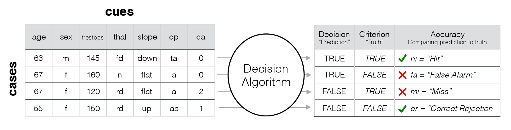
| Figure 1: The structure of a binary classification task. The data
underlying the task are arranged as a combination of cases (e.g.,
patients) and each case’s values on several cues (e.g., age,
sex, and various medical tests indicated by the labels trestbps,
thal, slope, cp, and ca).
Classification accuracy is evaluated by comparing the
algorithm’s decisions to the true criterion values. The goal of
the algorithm is to maximize correct decisions (hits and correct rejections),
while minimizing errors (misses and false-alarms). |
Despite their proven effectiveness, FFTs are still not used as often
as other decision algorithms. We believe that there are two key reasons for
this: First, while there are many tools in popular software packages
to create regression models and non-frugal decision trees, no such
tool currently exists to create FFTs. Although one could construct an FFT from data with a pencil, paper, and calculator using a heuristic tree
construction algorithm (Martignon et al., 2008), the process can be
tedious, especially for large datasets. Second, as complex,
computationally demanding algorithms, such as random forests and
support vector machines increase in popularity, simple algorithms like
FFTs are increasingly perceived as being outdated and inferior
prediction algorithms. This paper addresses both of these reasons by
introducing FFTrees (Phillips, Neth, Woike & Gaissmaier,
2017b), a toolbox written in the free and open-source R language (R
Core Team, 2016). As we will show, FFTrees makes it easy for
anyone to create, visualize, and evaluate FFTs that can compete with
the predictive power of more complex algorithms, while staying simple
and transparent enough for anyone to apply in real-world decision
environments.
The rest of this paper is structured as follows: Section 1 provides a
theoretical background on binary classification tasks, explains how
FFTs solve them and introduces a new class of “fan” algorithms for
constructing FFTs. Section 2 provides a 4-step tutorial on using the
FFTrees package to create and evaluate FFTs from
data. Finally, Section 3 presents simulation results comparing the
performance of the fan algorithms to existing FFT construction
algorithms and more complex algorithms such as logistic regression and
random forests.
2 Binary Classification Tasks
FFTs are supervised learning algorithms used to solve binary classification tasks. In a binary
classification task, a decision maker seeks to predict a
binary criterion value for each of a set of individual
cases on the basis of each case’s values on a range of
cues (a.k.a., features, predictors). The structure of the task
can be illustrated by a table in which each row represents a case,
each column represents a cue, and individual cells
represent cue values for specific cases.
Figure ?? illustrates data from a set of patients (cases),
where each case is characterized by their values on several
measures (cues), ranging from demographic variables, such as sex and
age, to biological measurements, such as cholesterol level and
other medical tests. The binary criterion is the patients’ heart disease status
which can either be true (i.e., having heart disease) or false
(i.e., not having heart disease). The true criterion values
are assumed to be unknown at the time of the decision and must be inferred from the cue
values. The goal of a decision maker presented with this information
is to accurately classify each case into one of two categories (i.e.,
as high-risk or as low-risk), and make an actionable decision
(i.e., send to the coronary care unit or a regular hospital bed) on
the basis of this classification.
Theoretically, this structure of a binary classification task is
captured by a variety of frameworks that range from the statistical
analysis of clinical judgments (e.g., Hammond, 1955; Meehl, 1954) and
comparisons between linear and non-linear regression models (Dawes,
1979; Einhorn & Hogarth, 1975) to the formalization of
discrimination performance in signal detection theory (SDT,
D. M. Green & Swets, 1966; Macmillan & Creelman, 2005). Practically,
the key question that arises in this context is: How to make good
classifications, and ultimately good decisions, based on cue
information? One way to do this is to use an algorithm.
A decision algorithm (for brevity, we use only the term
decision algorithm in this section, although the concepts apply
equally to classification algorithms) is a formal mapping between cue
values and a binary decision. We broadly distinguish between two
families of decision algorithms: compensatory and
non-compensatory. Compensatory algorithms, such as regression and random forests,
tend to use most, if not all, of the available cue information because
the value of one cue could potentially overturn the evidence given by
one or more other cues.1 By contrast, non-compensatory algorithms use only a
partial subset of all cue information, because the value(s) of one or
more cues can not be outweighed by any values of other
cues. That is, non-compensatory algorithms deliberately ignore
information because, once a decision is made based on some
information, no additional information can change the decision.
Non-compensatory algorithms can have both practical and statistical
advantages over compensatory algorithms. First, because they ignore
information, non-compensatory algorithms typically use less
information than compensatory algorithms. Second, because
non-compensatory algorithms typically use information in a specific,
sequential order, they can guide decision makers in gathering
information. For these reasons, non-compensatory algorithms are
especially well-suited to decision tasks for which information is
costly (in terms of time, money, or processing resources) and when
information must be gathered sequentially over time.
A prototypical non-compensatory algorithm is a decision tree
(Breiman, Friedman, Olshen & Stone, 1984; Quinlan, 1986, 1987). A
decision tree can be applied as a set of ordered, conditional rules in
the form “If A, then B” that are applied sequentially until a
decision is reached. Formally, a decision tree is comprised of a
sequence of nodes, representing cue-based questions,
branches, representing answers to questions, and leaves,
representing decisions. Decision trees are non-compensatory because,
once a decision is made based on some subset of the available
information (i.e., a higher node) no additional information (i.e., in
lower nodes) is considered. However, just because decision trees
ignore information does not guarantee that they are always
simple. Without appropriate restrictions a decision tree can contain
dozens of nodes forming a complex network of questions (Quinlan,
1986). When decision trees become overly complex, they become both
more difficult for people to understand and use. Moreover, complex
trees can be worse than simpler trees in predicting new data due to
statistical problem known as overfitting (as we will explain
below). This complexity problem is addressed by imposing strict
restrictions on the size and shape of decision trees. One of the most
restricted forms of a decision tree is a fast-and-frugal tree
(Martignon et al., 2008, 2003).
2.1 Fast-and-Frugal Trees (FFTs)
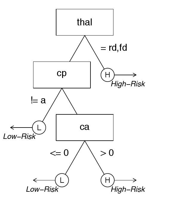
| Figure 2: A fast-and-frugal tree (FFT) for classifying patients as
either low or high-risk for heart disease based on up to three
cues. Each cue is contained in a node, represented as
rectangles. Decisions are made in leafs, represented as
circles. Branches represent answers to questions to cue–based questions. Branches connecting nodes to leafs are called exit
branches. One can use this tree to make a decision as follows: If a
patient’s thal (thallium scintigraphy result) value
is rd (reversible defect) or fd (fixed defect),
classify her as high-risk. If not, check her cp (chest pain
type) value. If this is aa (atypical angina), np
(non-anginal pain), or ta (typical angina), classify her
low-risk. If not, check her ca (number of major vessels
colored by flourosopy) value. If this is positive, classify her as
high-risk, otherwise classify her as low-risk. Note: After creating
the heart.fft object in the tutorial section “Using the
FFTrees package”, this plot can be generated by running
plot(heart.fft, stats = FALSE, decision.labels =
c("Low-Risk", "High-Risk"). |
Fast-and-frugal trees were defined by Martignon and colleagues as
decision trees with exactly two branches extending from each node,
where either one or both branches is an exit branch leading to a leaf (Martignon et al.,
2008, 2003). In other words, in an FFT one answer (or in the case of
the final node, both answers) to every question posed by a node will
trigger an immediate decision. Because FFTs have an exit branch on
every node, they typically make decisions faster than standard
decision trees (to avoid confusion, we refer to decision trees that
are not fast-and-frugal as standard) while simultaneously being
easier to understand and use.
Figure ?? presents an FFT designed to
classify patients as being at high or at low-risk for having heart
disease. The three nodes in the FFT correspond to the results of three
medical tests: thal indicates the result of a thallium
scintigraphy, a nuclear imaging test that shows how well blood flows
into the heart while exercising or at rest. The result of the test can
either be normal (n), indicate a fixed defect (fd),
or a reversible defect (rd). The second node uses the
cue cp, indicating a patient’s type of chest pain, which can
be either typical angina (ta), atypical angina (aa),
non-anginal pain (np), or asymptomatic (a). Finally,
ca indicates the number of major vessels colored by
fluoroscopy, a continuous x-ray imaging tool, whose values can range
from 0 to 3.
To classify a patient with the FFT, begin with the first node (the
parent node): If a patient’s thal value
is either rd or fd, then immediately classify
the patient as high-risk, ignoring all other information about the
patient. Otherwise, consider the next node: If a
patient’s cp value is aa, np,
or ta, then immediately classify the patient as
low-risk. Otherwise, consider the third and final node: If the
ca value is positive, classify the patient as high-risk,
otherwise classify the patient as low-risk.
As an example, consider a 65 year old, female patient with a
normal thal value, an atypical angina (cp = aa), and
a ca value of 1. To classify this patient, we first check if
her thal value is rd or fd. As it is not, we
check if her cp value is aa, np,
or ta. As this is the case, we classify her as low-risk and
do not consider any additional information.
For this patient, the non-compensatory FFT in
Figure ?? allows making a classifications
based on two cues without requiring a calculator. To classify this
patient using logistic regression—a common compensatory
classification algorithm—will not be as easy. Logistic regression
belongs to the larger family of general linear models that model
criterion values as a weighted sum of cue values and cue weights. That
is, each cue value is multiplied by a weight, added, and then
transformed by an equation to produce a continuous (probability)
prediction. A logistic regression solution for the heart disease
classification problem can be represented as
ln(p/1−p) = −2.76 + 1.53 · sex − 1.91 ·
cp_np − 2.12 · cp_ta + 0.02 ·
trestbps + 1.24 · ca, where p is the
estimated probability that a patient has heart disease. To use this
equation, we need to know four cue values (the patient’s sex,
cp, trestbps and ca values) multiply them
by a series of constants, sum them, and then transform the result with
an inverse-logit function. We can then compute, using an external
calculation device, the patient’s probability of having heart disease
as 70.7%. To finally classify the patient as having high or low-risk
for heart disease, we need to compare this probability to a
threshold. For example, using a threshold of 50%, we would classify
the patient as high-risk
2.2 Why use FFTs?
Why use FFTs rather than regression? FFTs have three key advantages,
based on their frugality, simplicity, and prediction accuracy (see
also Gigerenzer, Czerlinski & Martignon, 1999; Martignon et al.,
2008, 2003). First, FFTs tend to be both fast and frugal as they
typically use very little information. The FFT for diagnosing heart
disease in Figure ?? requires a maximum of
three cue values, but as the previous example suggests, FFTs
frequently make decisions after considering fewer cue values, as every
node has an exit branch that can trigger an early decision. By
contrast, regression typically requires more information and thus
takes longer to implement. The logistic regression heart disease
algorithm always requires four cue values, as the patient’s value on
any one of these cues could potentially change the final
decision. Thus, FFTs are heuristics by virtue of ignoring
information (Gigerenzer & Gaissmaier, 2011). The fact that heuristics
like FFTs ignore information does not necessarily imply that they will
perform worse than slower and less frugal algorithms. As heuristics
are tools that tend to work well under conditions of uncertainty (Neth
& Gigerenzer, 2015), it is an empirical question whether an FFT’s
gain in speed and frugality reduces its predictive accuracy relative
to regression (Gigerenzer, Todd & the ABC Research Group, 1999).
Second, FFTs are simple and transparent, allowing anyone to easily
understand and use them. The heart disease FFT in
Figure ?? can be quickly communicated,
learned, and applied either by a computer or “in the head”. By
contrast, the regression variant requires training to understand, and
usually a calculator to implement. The simplicity and transparency of
FFTs make them particularly useful in domains where decision rules
need to be quickly understood, implemented, communicated, or taught to
decision makers.
Finally, FFTs can make good predictions even on the basis of a small
amount of noisy data because they are relatively robust against
a statistical problem known as overfitting. As we describe
below, overfitting occurs when an algorithm has systematically lower
accuracy in predicting new, unseen data compared to fitting old, known
data. In contrast to regression (particularly in its classic,
non-regularized form), FFTs tend to be robust against overfitting,
and have been found to predict data at levels comparable with
regression (Martignon et al., 2008; Woike, Hoffrage & Martignon,
2017).
| Figure 3: A 2 x 2 confusion table and accuracy statistics used to
evaluate a decision algorithm. Rows refer to the frequencies of
algorithm decisions (predictions) and columns refer to the
frequencies of criterion values (the truth). Cells hi and
cr refer to correct decisions, whereas cells fa and
mi refer to errors of different types. Five measures of
decision accuracy are defined in terms of cell frequencies. |
2.3 Why are FFTs not more popular?
Given these advantages of FFTs, it is puzzling that FFTs are used far
less than other classification algorithms such as regression. We
believe that there are three main reasons for this: First, people use
tools that are accessible and easy to use, and most standard software
packages do not contain algorithms for creating FFTs. Second, people
often evaluate decision algorithms based on their ability to fit known
data, rather than their ability to predict new data. This is both
theoretically and statistically problematic, as it favors overly
complex models that are prone to fitting random noise (see Gigerenzer
& Brighton, 2009; Pitt & Myung, 2002; Roberts & Pashler,
2000). Consequently, focusing on fitting punishes simple algorithms
like FFTs that tend to be worse than complex algorithms at fitting
past data, but as good, if not better, at predicting new data (see
Gigerenzer & Brighton, 2009; Walsh, Einstein & Gluck, 2013, for a
discussion of the bias-variance dilemma and the robustness of
heuristics).
The third reason against a wider adoption of FFTs is skepticism that
something as simple as an FFT can be as accurate as a more complex
algorithm. This skepticism is partly due to a suspected trade-off
between information frugality and prediction accuracy. According to
this trade-off, the more information an algorithm uses, the
more accurate it will be—in other words: “more is better.” For
someone subscribing to the more-is-better principle, the idea that a
simple FFT that explicitly ignores information could be as accurate as
a compensatory decision that uses all or most of the available
information seems preposterous. But despite its intuitive
plausibility, when it comes to building predictive models, the “more
is better”-mantra is often mistaken (Dawes, 1979; Gigerenzer & Brighton, 2009;
Gigerenzer & Goldstein, 1996). Several studies comparing the accuracy
of simple FFTs to more complex decision algorithms have found that
FFTs can closely match, and even outperform more complex
algorithms in predicting new data in domains ranging from medical and
legal to financial and military decision making (see Aikman et al.,
2014; Dhami & Ayton, 2001; Fischer et al., 2002; 205 L. Green &
Mehr, 1997; Jenny et al., 2013; Keller & Katsikopoulos, 2016;
Martignon et al., 2008; Wegwarth et al., 2009, for examples). These
results have shown that less can be more, and that FFTs need not
necessarily sacrifice accuracy for the sake of simplicity, clarity, or
speed. Rather, FFTs can be accurate because of their
simplicity, not in spite of it (see Gigerenzer & Gaissmaier, 2011,
for additional less-is-more effects).
In the following section we explain how to quantify the accuracy and
efficiency of a decision algorithm, and show how FFTrees
creates FFTs that are simultaneously fast, frugal, and accurate. We then present a 4-step tutorial on how to construct and visualize
FFTs from data using FFTrees. Finally, we conduct a series
of simulations on 10 real-world datasets to compare the prediction
performance of FFTrees to several popular decision
algorithms.
2.4 Evaluating and constructing FFTs
To reiterate, the decision problems we address are binary
classification tasks for which data can be organized in
a table (as in Figure ??), where several
cases are characterized by their values on several cues.
Cues can either be numeric, such as age,
or nominal, such as sex. The criterion is a column of binary
values—either positive (True or 1) or negative (False or 0)—
that one wishes to predict.
In the present paper, we focus on building prescriptive FFTs that
predict criterion values for any kind of data, whether it is
behavioral data representing actual decisions, such as a doctor’s diagnoses,
or non-behavioral data representing true states of the world, such as
a patient’s health status.
As we will return to in the Discussion, we do not claim that FFTs,
specifically those created by FFTrees, are necessarily good
(or bad) models of the decision process underlying behavioral data.
The purpose of FFTs built by FFTrees is to efficiently and
accurately predict binary criterion values on the basis of cues,
without claiming that the tree does, or does not, capture the original
data generating process.
2.4.1 Measuring accuracy
To define the accuracy of a decision algorithm, we contrast its
decisions with true criterion values in a confusion table like
the one shown in Figure ??. A confusion table
cross-tabulates the decisions of the algorithm (rows) with true
criterion values (columns) and contains counts of observations for all
four resulting cells. Counts in cells hi and cr refer to
correct decisions due to the match between predicted and criterion
values, whereas counts in cells fa and mi refer to
errors due to a mismatch between predicted and true criterion
values. Both correct decisions and errors come in two types:
Cell hi represents hits, positive criterion values
correctly predicted to be positive, and cell cr represents
correct rejections, negative criterion values correctly
predicted to be negative. As for errors, cell fa represents
false alarms, negative criterion values erroneously predicted
to be positive, and cell mi represents misses, positive
criterion values erroneously predicted to be negative. Given this structure, a decision algorithm aims to maximize
frequencies in cells hi and cr while minimizing those in
cells fa and mi.
There are many different ways to combine the cell frequencies in a
confusion table into aggregate measures of accuracy. We focus on five
measures: sensitivity (sens), specificity (spec),
overall accuracy (acc), weighted accuracy (wacc),
and balanced accuracy (bacc). The first two measures define
accuracy separately for cases with positive and negative criterion
values. An algorithm’s sensitivity (a.k.a., hit-rate) is
defined as sens = hi / (hi + mi) and represents the
percentage of cases with positive criterion values that are correctly
predicted by the algorithm. Similarly, an algorithm’s
specificity (a.k.a., correct rejection rate, or the compliment
of the false alarm rate) is defined as spec = cr / (fa + cr)
and represents the percentage of cases with negative criterion values
correctly predicted by the algorithm. The next three measures define
accuracy across all cases. Overall accuracy is defined as the
overall percentage of correct decisions
acc = (hi + cr) / (hi + fa + mi + cr), ignoring the
difference between hits and correct rejections.
Although overall accuracy is an important and useful measure, it can
be misleading and must be interpreted relative to the base rate of the
criterion. For instance, in a dataset with a low base rate of 1%
(e.g., 100 cases and only one case with a positive criterion value), a
baseline algorithm that simply predicts every case to be
negative would achieve an overall accuracy of 99%. Thus, baseline
algorithms can have a high overall accuracy without being very useful
because they do not distinguish between positive and
negative cases. An extremely liberal baseline algorithm that always
predicts “True” will never miss and thus have a seemingly desirable
sensitivity of 100%. But this comes at the cost of many false
alarms and a dismal specificity of 0%. By contrast, an extremely
conservative algorithm that always predicts “False” will maximize
correct rejections and exhibit an impressive specificity of 100%, but
at the cost of many misses and a sensitivity of 0%. Indeed, there is
an inevitable sensitivity–specificity trade-off in most
classification tasks, such that an increase in one measure corresponds
to a decrease in the other (Macmillan & Creelman, 2005). The shape of
this trade-off can be expressed by a receiver operating
characteristic (ROC) curve like the one in Figure ??, which
shows the sensitivity-specificity trade-off of 7 different algorithms
applied to the same data set. Here, algorithms with higher
specificities tend to have lower specificities, and vice-versa.
Different tasks and decision maker preferences can influence the
extent to which sensitivity should be weighted relative to
specificity. For example, consider the head of airport security who
needs to construct a decision algorithm for bag screening, where any
bag can be either truly safe (i.e., does not contain a safety threat)
or unsafe (i.e., does contain a threat). To construct a good decision
algorithm, she needs to take into account the relative cost of a
false-alarm (falsely identifying a safe bag as unsafe), to the cost of
a miss (falsely identifying an unsafe bag as safe). But what are these
costs? There is no definitive answer to this question because the
relative costs of both errors depend on the specific decision made for
each case after it is classified. For example, consider the following
two decision rules: “If a bag is classified as unsafe, hold it for an
additional 30 minutes of manual screening to be certain of its
contents. If a bag is classified as safe, let it pass without
additional screening.” Here, the cost of a miss is the potential
loss of life due to a missed threat, while the cost of a false-alarm
is an additional 30 minutes of screening time. Clearly, the cost of a
miss in this scenario exceeds the cost of a false-alarm and thus calls
for a decision algorithm that prioritizes sensitivity over
specificity.2 As this example shows, a good decision algorithm
should be able to balance sensitivity and specificity as a function of
the specific error costs of a domain.
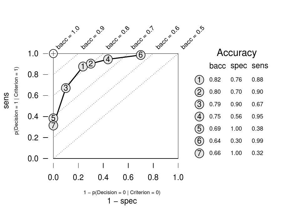
| Figure 4: A receiver operating characteristic (ROC) curve illustrating
the trade-off between sensitivity (sens) and specificity
(spec) in classification algorithms. As sensitivity
increases, specificity decreases (i.e., 1 − spec
increases). Balanced accuracy (bacc) is the average of
sensitivity and specificity. Ideal performance (bacc =
1.0), is represented by the cross in the upper-left corner. The
numbered circles in the plot represent the accuracy of 7 different
algorithms with different trade-offs between sensitivity and
specificity. Their numbers represent the rank order of algorithm
performance in terms of their bacc values. (Note: The
circles correspond to the fan of 7 FFTs that will be created by the
ifan algorithm for the heart disease dataset in the tutorial.) |
To quantify how an algorithm balances sensitivity and specificity, we
use weighted accuracy. Formally, weighted accuracy is defined
as wacc = w · sens + (1−w) · spec,
where w (labeled sens.w in FFTrees) is a parameter
between 0 and 1 that specifies how sensitivity is weighed relative to
specificity. In decision tasks where sensitivity is more important
than specificity (like threat detection in airport screening),
wacc could be calculated with a value of w larger than 0.5.
In cases where both measures are equally important, the
sensitivity weight w can be set to 0.5. In this special case,
weighted accuracy is called balanced accuracy (bacc).
There are many alternative measures to quantify the accuracy of an
algorithm across all cases, most notably d-prime (d’) and area under the
curve (AUC). For simplicity, we focus on wacc (with
bacc as a special case) for the remainder of this paper, as it
provides a simple way to account for both false-alarms and misses,
while using an interpretable scale of values ranging from 0 to 1
(where 0 indicates no accuracy, and 1 equals perfect accuracy, see
Figure ??).
2.4.2 Measuring speed and frugality
Although prediction accuracy is an important characteristic of an
algorithm, algorithms should also be evaluated based on their
efficiency. If two algorithms have similar accuracy, but one is more
efficient than the other, then the more efficient algorithm should be
preferred because it will be cheaper (in terms of time and/or money)
to implement, while being easier to understand, and communicate. For
this reason, in addition to measuring an algorithm’s accuracy, we also
measure its efficiency in terms of speed and frugality.
Previous FFT literature has operationalized an algorithm’s
speed and frugality with a single measure, usually as the
number of cues used when implementing the algorithm, averaged across
cases (e.g., Dhami & Ayton, 2001; Gigerenzer & Goldstein, 1996;
Jenny et al., 2013). By contrast, we measure speed and frugality with
two distinct measures that separate how rapidly an algorithm reaches a
conclusion (its speed) from how much information it ignores (its
frugality).
We quantify an algorithm’s speed with the measure mean
cues used (mcu), the average number of cue values used in
making a decision, averaged across all cases. For example, an
algorithm that uses 1 cue to make a decision for half of the cases,
and 2 cues for the remaining half, would have an mcu value
of 1.5. This is the same measure used in previous FFT research as an
overall measure of both speed and frugality.
We separately define an algorithm’s frugality with the measure
percent cues ignored (pci), defined as 1 minus an
algorithm’s mcu divided by the total number of cues in the
dataset (i.e., the maximum possible mcu value). This measure
quantifies the percentage of information an algorithm ignores
when it is implemented on a specific dataset. For example, in a
dataset with 10 cues, an algorithm that uses 1 cue value to make a
decision for every case (resulting in an mcu value of 1)
would ignore 9 cue values for every case, resulting in a pci
value of 1 − 1/10 = 90%. By contrast, an algorithm that uses 9 cue
values to classify every case would ignore very little information,
and thus have a pci value of 1 − 9/10 = 10%. Thus, the
more data an algorithm ignores (i.e., the higher its pci
value), the more frugal it is.
It is important to distinguish between an algorithm’s speed (measured
by mcu) and its frugality (measured by pci) for the
following reason: A fast algorithm is not necessarily frugal, nor is
a frugal algorithm necessarily fast. For example, when presented with
a large dataset containing 100 cues, an algorithm that uses 10 cues on
average (mcu = 10) to classify each case would, by most
standards, not considered to be very fast. However, the algorithm
would nonetheless be quite frugal (pci = 90%) relative to
a complex algorithm that uses all available information. By contrast,
the same algorithm applied to a smaller dataset that includes only the
10 cues actually used by the algorithm would no longer be frugal
(pci = 0%) because it does not ignore any
information. This example illustrates a second important point beyond
the distinction between frugality and speed: While some algorithms
will be faster and/or more frugal than others on average, the speed
and frugality of an algorithm also depend on the data to which it is
applied. In other words, an algorithm that is fast and frugal for one
dataset could be slow and wasteful for another. For this reason, we
consider and provide both measures when evaluating and comparing
algorithms across datasets.
2.4.3 Training (fitting) vs. testing (prediction)
Regardless of the specific accuracy and efficiency measures used, a
decision algorithm must always be evaluated in reference to one of two
phases in the modeling process. In the training phase (a.k.a.,
fitting phase) true criterion values are provided to the
algorithm so that it can adjust its free parameters to the specific
decision task. In regression, these parameters take the form of
regression weights. In an FFT, they are its cues, decision thresholds,
cue order, and exits. In the testing phase (a.k.a.,
prediction phase) the algorithm must predict the criterion
values of new data (i.e., data not used during training) by using the
specific parameter values derived during the training phase. Thus, the
purpose of the testing phase is to evaluate an algorithm’s ability to
make true predictions for data that it has not encountered before.
There is an important reason why one should always distinguish between
an algorithm’s accuracy in training and testing: Algorithms can have
systematically higher accuracy in training data compared to their
accuracy in testing data. The reason for this discrepancy is a
statistical phenomenon known as overfitting (James et al.,
2013). To understand overfitting, it is helpful to view a dataset as
a combination of signal and noise, where the signal is a stable and
systematic pattern in the data and noise is unpredictable
variability due to measurement error or other random influences. As
noise, by definition, cannot be predicted, while signal can, a good
decision algorithm should detect and model signal and ignore noise
(Gigerenzer & Brighton, 2009; Kuhn & Johnson, 2013; Silver,
2012). Generally speaking, overfitting occurs when an algorithm
mistakes noise in a dataset for a signal, and as a result, changes its
parameters to accommodate noise rather than (correctly) ignoring
it. This leads to an inflated level of accuracy that can not possibly
be maintained when predicting future data that will inevitably be
contaminated with unpredictable noise. When decision makers want to
maximize their ability to predict new data, decision algorithms should
be evaluated based on their prediction accuracy in the testing phase
rather than on their fitting accuracy in the training phase. The
robustness of a decision algorithm can then be expressed in
terms of its resistance to overfitting: An algorithm that avoids
confusing noise for a signal is robust in the sense that it achieves
similar levels of accuracy for training and testing data. Equipped
with these measures and conceptual distinctions, we can now describe
the algorithms available in the FFTrees package that can be
used to construct FFTs.
2.5 FFT construction algorithms
Constructing an FFT refers to the training phase in which the
parameters of an FFT are tailored to a specific dataset. An FFT
construction algorithm must solve the following four tasks (but not
necessarily in this order): 1. Select cues; 2. Determine a decision
threshold for each cue; 3. Determine the order of cues; and
4. Determine the exit (positive or negative) for each cue. Each of
these tasks is critical in constraining how, and how well,
an FFT will perform.
Two FFT construction algorithms, max and zig-zag, have
been proposed and tested by Martignon and colleagues (Martignon et
al., 2008, 2003; Woike et al., 2017). Both algorithms use several
heuristics that simplify the process of tree construction. The basic
steps in each algorithm are as follows: First, to determine the
decision thresholds of numeric cues, both algorithms use the observed
median value of numeric cues rather than using a value that optimizes
any performance criteria. Second, the individual, marginal
positive predictive and negative predictive
validities3
of each cue are calculated, ignoring any potential dependencies
between cues. For the max algorithm, cues are ranked in order of the
maximum value of their positive and negative validities. Cues with
higher positive than predictive validities are then assigned positive
exits, while those with higher negative than positive predictive
validities are given negative exits.
In contrast to max, zig-zag determines the exit direction for each
node before determining cue order. Specifically, after the first node
is given a positive or negative exit, all sequential nodes then are
given alternating exits.4 Once exits are determined, zig-zag
recursively assigns the cue with the highest positive predictive value
to the next node with a positive exit, and the cue with the highest
negative predictive value to the next node with a negative exit.
The max and zig-zag algorithms have been shown to produce FFTs that
can compete with logistic regression and standard decision trees in
predictive accuracy (Martignon et al., 2008). Moreover, because they
use several simplifying heuristics throughout the construction
process, they require very few calculations and can in principle be
implemented with a pencil and paper.
Although max and zig-zag are simple and effective, they lack two
features that can make them unsuited for certain decision
problems. First, they do not have sensitivity and specificity
weighting parameters. This means that they cannot create FFTs tailored
to decision tasks where false-alarms are more (or less) costly than
misses. Second, the algorithms do not have explicit size restrictions
or a process of removing nodes from a tree (a.k.a., “pruning”). This
means that max and zig-zag create FFTs that use all cues in a
dataset, regardless of whether or not the cues are actually used in
classification. In datasets with only a few cues, this does not pose a
problem; however, in datasets with dozens or even hundreds of cues,
this can lead to extremely long trees containing nodes that may never
be used in practice.
To address the sensitivity weighting and tree size issues present
existing FFT construction algorithms, we introduce a new class of
algorithms called fan with two variants: ifan and
dfan. These algorithms account for different sensitivity and
specificity weights by taking advantage of the effect of an FFT’s
exit structure, its particular sequence of negative and
positive exits, on its balance between sensitivity and specificity. By
definition, every node in an FFT must have either a negative or a
positive exit (or both in the case of the final node). Martignon et
al. (2008) and Luan, Schooler, and Gigerenzer (2011) have shown that
the exit structure of an FFT can dramatically affect its balance
between sensitivity and specificity. For example, an FFT with either
all positive or all negative exits (except for the last node which
must contain both a positive and a negative exit), known as a
rake (Martignon et al., 2003), tends to maximize one metric to
the detriment of the other. An FFT with only positive exits until the
last node, a “positive-rake”, exhibits high sensitivity at the
expense of low specificity because every node in the tree can trigger
a positive decision. By contrast, an FFT with only negative exits
until the last node, a “negative-rake”, exhibits high specificity at
the expense of low sensitivity because every node in the tree can
trigger a negative decision. In contrast, an FFT with alternating
positive and negative exit directions, known as a “zig-zag” tree,
will tend to balance sensitivity and specificity. Thus, just as a
judge can adjust her decision criterion in the signal detection theory
framework to shift her balance in decision errors, so can an FFT
change its exit structure (Luan et al., 2011).
Inspired by the role an FFT’s exit structure has on its error balance,
the ifan and dfan algorithms explore a virtual “fan” of several FFTs
with different exit structures and error trade-offs, ranging from
negative-rakes, to zig-zag trees, to positive-rakes. After the fan is
created, the algorithms select the tree with the exit structure that
maximizes the statistic the unique error trade-off (i.e., weighted
accuracy) desired by the decision maker. They also have parameters
that both limit the size of FFTs, and remove nodes deemed to be
unnecessary because they either do not classify enough cases (the
default), or because they do not substantially increase accuracy.
Full descriptions of the ifan and dfan algorithms are presented in
the Appendix. Here, we describe the algorithms’ rationale more
generally. The ifan algorithm works as follows: Like max and zig-zag,
ifan first calculates a decision threshold t for each cue. For
numeric cues, thresholds are single values, whereas for factors (i.e.,
nominal or character cues), thresholds are sets of one or more factor
values. Thresholds are also combined with decision directions
to indicate how the threshold would be used to make a positive
classification decision. For example, in using the cue age to
predict the presence of heart disease risk, a threshold and direction
could be > 65, indicating that people over the age of 65 are
predicted to be at high risk for having heart disease. Unlike max and
zig-zag, ifan is not restricted to using cue medians as thresholds for
numeric cues. Instead, it tests several different thresholds (for
numeric cues, the default value is 20) to find one that that maximizes the
cue’s accuracy goal.chase (by default, goal.chase =
bacc) when applied to entire training dataset and ignoring all
other cues.
Next, ifan ranks the cues in order of their maximum values of
goal (by default, goal = bacc).5 It
then selects the top max.levels cues (by default,
max.levels = 4), and discards all remaining cues. The
algorithm then creates a set of 2max.levels−1 FFTs with
these cues, keeping their order constant, using all possible exit
structures. This set of trees represents the “fan”. For example,
the seven points in Figure ?? represent seven different
FFTs within one fan. Next, the algorithm removes any lower nodes in
the FFTs that classify fewer than stopping.par (by default,
stopping.par = 10%) percent of the data.6 If lower
nodes are removed, the final remaining node is forced to have both a
positive and a negative exit branch. Due to the option of removing
low-data nodes, the final number of cues in an FFT may be lower than,
but cannot exceed max.levels.
Once the set of FFTs has been created, ifan selects the tree with the
highest goal value. By default, its goal is weighted
accuracy (wacc), calculated with a sensitivity weight
parameter (sens.w) specified by the user. To be clear, by
default, the value of sens.w does not change how the set of
FFTs are constructed (as long as goal.chase = bacc): rather,
it changes which specific tree in the set of FFTs with different exit
structures is selected to make classification
decisions.7
A key restriction that ifan shares with max and zig-zag is that it
ignores potential interactions between cues—both in their decision
thresholds and their ranked accuracy. That is, these algorithms
calculate decision thresholds and then rank cues based on their
marginal accuracy. Does assuming cue independence hurt the performance
of an algorithm? Intuition suggests that it would, as one can easily
imagine scenarios where cues are not independent. For example, in
diagnosing heart disease, we could hypothesize an interaction between
weight and sex such that relationship between
weight and heart disease is, substantially and reliably, not
the same for men and for women. If so, a decision algorithm would make
better predictions by calculating a different decision threshold for
the weight of men versus women. Indeed, most algorithms for
constructing standard decision trees (such as ID3 and C4.5, Quinlan,
1986, 1993) implicitly take cue interactions into account by
sequentially calculating new thresholds during tree
construction. However, one must be careful in assuming cue dependence
for following reason stated by Martignon et al.: “the fact that cue
interactions can exist […], does not imply that they must exist;
it says nothing about the frequency of their occurrence” (2003,
p. 210). The reason why one should be careful in assuming cue
interactions is that this assumption can come at a cost: If an
algorithm that takes cue interactions into account is applied to a
dataset where cue interactions either do not exist, or cannot be
reliably estimated from training data, then the algorithm is likely to
overfit the training data and can lead to poorer predictions than an
algorithm that explicitly ignores cue interactions (see Gigerenzer &
Brighton, 2009; Martignon & Hoffrage, 2002, for a more detailed
discussion). In other words, algorithms that routinely incorporate
cue interactions may commit false-alarms in detecting (and subsequently
predicting) cue interactions that may be spurious or unreliable. For
this reason, many successful heuristics (such as as take-the-best,
Gigerenzer & Goldstein, 1996) and FFT construction algorithms (such
as max and zig-zag, Martignon et al., 2008, 2003) explicitly ignore
cue interactions to reduce both processing time and the risk of
overfitting.
In decision domains where substantial interactions between cues are
likely to exist and can reliably be measured in training data, FFT
construction algorithms that assume dependencies between cues may
provide better predictions than algorithms that do not. To provide
users with a fitting FFT construction tool for such tasks, we
provide a variant called dfan that does not assume cue
independence. The dfan algorithm starts like ifan
by ranking cues based on goal (by default,
goal = bacc). But instead of calculating cue thresholds based
on all cases and ranking cues based on their accuracy only once, it
iteratively re-calculates cue thresholds and accuracies based on
the subsets of cases that occur dynamically as the FFT is being
constructed. This allows dfan to detect and exploit cues that may
exhibit poor overall accuracy, but are highly predictive for specific
subsets of cases partitioned by other cues.
In the next section, we provide a tutorial for creating, evaluating,
and visualizing FFTs with the FFTrees package. We illustrate
each step with example code from a dataset on heart disease (Detrano
et al., 1989), which is included in the FFTrees package, and
ultimately arrive at the exact FFT for predicting heart disease
presented in Figure ??, and the ROC curve in
Figure ??. While we use the heart disease data throughout,
we remind the reader that FFTrees is in no way restricted to
medical data and can be used to model any dataset with a binary
criterion.
3 FFTrees Tutorial
FFTrees should be used with versions 2.1.0 of R or greater. R
can be downloaded for free from https://cloud.r-project.org. We
recommend also using the RStudio programming environment from
https://www.rstudio.com/products/rstudio/. Reproducible code
corresponding to the tutorial is provided in Figure
?? and is also available at
https://osf.io/m726x/ (Phillips, Neth, Woike & Gaissmaier,
2017a). The code and documentation presented here is valid for
FFTrees version 1.3.2, but should also be valid for future
package versions. The latest developer version of FFTrees is
available at http://www.github.com/ndphillips/FFTrees. We
welcome bug reports, feature requests, and code contributions at
http://www.github.com/ndphillips/FFTrees/issues.
# ------------------------------------------------------------
# 4 Steps to create and visualize a fast-and-frugal tree (FFT)
#  predicting heart disease using FFTrees
# ------------------------------------------------------------

# Step 0: Install the FFTrees package (only necessary once)
install.packages("FFTrees")

# Step 1: Load the FFTrees package and open the package guide
library("FFTrees")                # Load the package
FFTrees.guide()                   # Open the package guide

# Step 2: Create FFTs from training data and test on testing data
heart.fft <- FFTrees(formula = diagnosis ~ ., # Criterion
                     data = heart.train,      # Training data
                     data.test = heart.test,  # Testing data
                     main = "Heart Disease",  # Optional labels
                     decision.labels = c("Low-Risk", "High-Risk"))

# Step 3: Inspect and summarize FFTs
heart.fft            # Print statistics of the final FFT
inwords(heart.fft)   # Print a verbal description of the final FFT
summary(heart.fft)   # Print statistics of all FFTs

# Step 4: Visualize the final FFT and performance results
# a) plot final FFT applied to test data:
plot(heart.fft, data = "test")

# b) plot individual cue accuracies in ROC space:
plot(heart.fft, what = "cues")
| Figure 5: Complete, reproducible code showing four basic steps to create, visualize, and evaluate FFTs predicting heart disease with FFTrees. The datasets used for training (heart.train) and testing (heart.test) are included in FFTrees
and an expanded tutorial for this code is available in the package by evaluating vignette("FFTrees_heart"). A link to a video tutorial corresponding to this code is also available at https://osf.io/m726x/ (Phillips et al., 2017a). |
3.1 Step 1: Install the FFTrees package
FFTrees can be installed from CRAN by evaluating
install.packages("FFTrees"). Once the package has been
installed on a computer, it does not need to be installed again
(except to check for a more recent version). Once the package is
installed and loaded, a package guide containing instructions and
examples can be opened by running FFTrees.guide().
3.2 Step 2: Create FFTs with FFTrees()
The main function for creating FFTs is FFTrees(). The
function has two mandatory arguments formula and
data. The formula argument should be of the form
formula = criterion ~ a + b + ... specifying
the criterion (criterion) and one or more cues (a, b,
...) to be considered, but not necessarily used in the FFT.
For example, including formula = diagnosis
~ sex + age will create FFTs predicting diagnosis
that only consider the cues sex and age. One can
also use the generic formula = criterion
~ . notation, which allows to consider
all cues in the training data. Unless there are specific cues in the
training data that should, or should not, be considered, we recommend
using the generic formula notation.
The second mandatory argument to the FFTrees() function is
data, a training dataset containing all cues specified in
formula. The training data should be stored as a data frame
consisting of m rows (cases) and n columns. One of the columns
must be the binary criterion specified in the formula
argument. Although there are no explicit restrictions on the number
and classes of cues, we recommend not including factor cues with many
(i.e., more than 20) unique cue values, as this can lead to long
processing times and potential overfitting. Missing values are
(currently) not permitted.
The optional data.test argument allows specifying a testing
dataset used to test the prediction performance of the tree. In the
absence of separate training and test datasets, one can use the
train.p = p argument to automatically split the original
training data (specified with the data argument) into
separate training and test subsets. Setting train.p = p will
split all cases contained in data into a proportion
p used for training and 1−p for testing. For
example, setting train.p = .10 will randomly split the
original data into a 10% training set, and a 90% testing
set.8
Additional optional arguments include main and
decision.labels, with which users can specify verbal
labels for the dataset and/or decision outcomes. These arguments
are passed to other functions such as plot(). There are
several additional optional arguments one can use to customize how
the trees are constructed. The algorithm argument specifies
the FFT construction algorithm. The default algorithm is ifan (i.e.,
algorithm = ‘‘ifan’’), however, the user can also specify
‘‘max’’, ‘‘zig-zag’’, or ‘‘dfan’’ to create
FFTs using one of these algorithms. For the fan algorithms, the
arguments max.levels and sens.w, additionally
control tree size and sensitivity weights (for the ifan and dfan
algorithms only), while goal and goal.chase specify
which accuracy statistic is maximized when growing the tree(s), and
selecting the final tree, respectively. Additional details about these
and other arguments are provided in the package documentation.
3.3 Step 3: Inspect FFTs
The FFTrees() function returns an object of the
FFTrees class. An overview of the trees contained in the
object is available in three ways: by printing the object to the
console, by summarizing it with summary(), or by obtaining a
verbal description of it with inwords(). Most of the
following functions will automatically return details of the FFT with
the highest weighted accuracy (wacc) in the training
data. However, users can also return results from other trees in
the fan by specifying an integer value in the tree argument.
Printing an FFTrees object (i.e., evaluating the object by
its name) displays basic statistics—including the number of cases and
metrics for accuracy, speed, and frugality in training vs. testing
data—to the console (see Table ??).
Applying the summary() function to an FFTrees object
returns detailed information on each of the FFTs, including their
cues, decision thresholds, exits and exit directions, as well as
accuracy and efficiency statistics.
Finally, applying the inwords() function to an
FFTrees object returns a verbal description of the tree. For
example, evaluating inwords(heart.fft) on the heart disease
FFTrees object returns the sentence: “If thal =
{rd, fd}, predict High-Risk. If cp != {a}, predict
Low-Risk. If ca <= 0, predict Low-Risk, otherwise, if
ca > 0, predict High-Risk.”
| Table 1: Printing an FFTrees object provides summary statistics on the created FFTs, selects the FFT with the highest weighted accuracy (wacc) in training and shows its performance measures for training and testing data. |
| Heart Disease |
| 7 FFTs predicting diagnosis (Low-Risk vs. High-Risk) |
| FFT #1 contains 3 cues: {thal, cp, ca} |
| Measure | | Label | | Training | | Testing |
| cases | | n | | 150 | | 153 |
| speed | | mcu | | 1.74 | | 1.73 |
| frugality | | pci | | 0.88 | | 0.88 |
| accuracy | | acc | | 0.80 | | 0.82 |
| weighted accuracy | | wacc | | 0.80 | | 0.82 |
| sensitivity | | sens | | 0.82 | | 0.88 |
| specificity | | spec | | 0.79 | | 0.76 |
3.4 Step 4: Visualize and evaluate FFTs
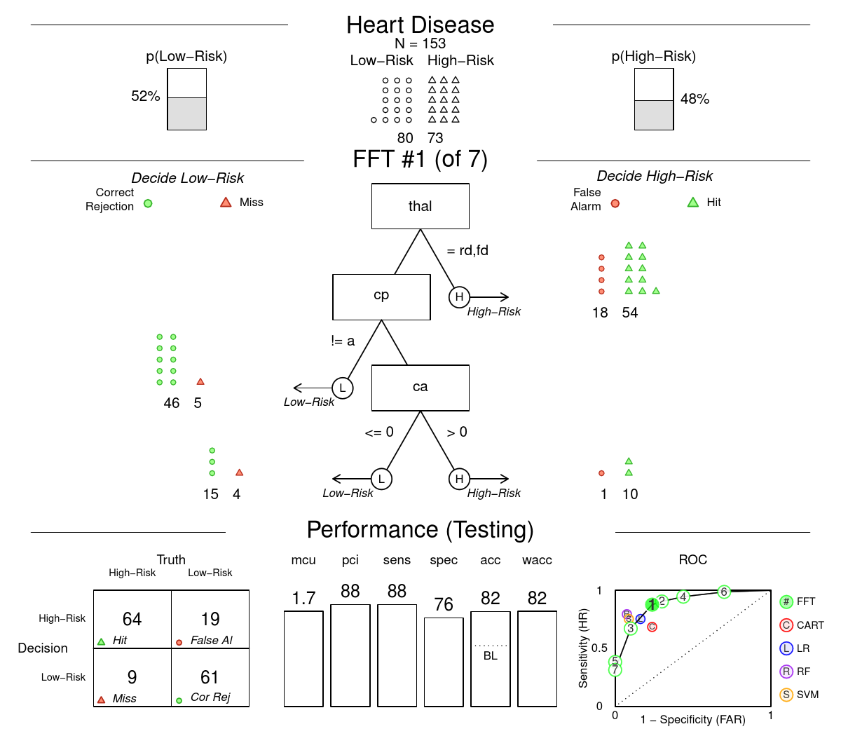
| Figure 6: Visualization of an FFTrees object created by plot(heart.fft, data = "test"). The top panel shows information about the dataset, including the frequencies and base rates of negative and positive criterion classes. The middle panel contains the FFT and icon arrays showing the the
number and accuracy of cases classified at each node. This particular
FFT’s interpretation has been described above (on
p. ?? and in Figure ??).
The bottom panel shows the FFT’s cumulative classification
performance, including a confusion table and levels for a
range of statistics. The bottom right plot shows the
performance of all seven FFTs created by the FFTrees()
function in ROC space (green circles with numbers correspond to
FFTs). The FFT currently being plotted is highlighted (here, FFT #1,
with the highest weighted accuracy in training). Additional points in
this plot correspond to the performance of competing classification
algorithms (see Simulation section): standard decision trees (CART),
logistic regression (LR), random forests (RF), and support vector
machines (SVM). In this case, FFT #1 has a higher sensitivity than
competing algorithms, but at the cost of a lower
specificity. Additionally, FFT #1 dominates CART in this example by
having a higher sensitivity and comparable specificity. |
To visualize a specific FFT contained in an FFTrees object,
as well as its associated accuracy statistics when applied to either
the training or testing data, apply the generic plot()
function to the object. By default, the FFT with the highest weighted
accuracy (wacc) in the training data is shown. Figure
?? shows heart disease FFT applied to the
testing data. Colored icon arrays (Galesic, Garcia-Retamero &
Gigerenzer, 2009) illustrate how the tree made decisions for all 153 cases
in the testing data. The bottom panel provides cumulative
accuracy statistics. Additionally, the accuracies of each tree in the
fan of seven FFTs generated by ifan are visible in the ROC curve in
the bottom-right of the plot (these are identical to the points in
Figure ??). Using the additional arguments tree
and data allows users to select which FFT in the fan is
plotted, and which dataset (training or testing) is displayed.
To visualize the marginal accuracy of every cue in the dataset,
include the what = ‘‘cues’’ argument when plotting an
FFTrees object. This option illustrates the individual,
marginal accuracies for each cue in ROC space.
Figure ?? shows the resulting plot for the heart disease
data. Inspecting the graph reveals that the three cues (thal,
cp, ca) used in FFT #1 (shown in
Figure ??) have the highest individual balanced
accuracies. Note that this is to be expected as the ifan
algorithm explicitly selects and ranks cues by this
statistic by default. Figure ?? also shows that the two next best
cues are oldpeak and slope. This information can
be useful in guiding a top-down process of future FFT
construction. For example, if those cues were of particular interest,
one could build a new FFT with these cues by evaluating
heart2.fft <- FFTrees(formula = diagnosis ~
thal + oldpeak + slope, data = heart), and then compare the
performance of the two trees.
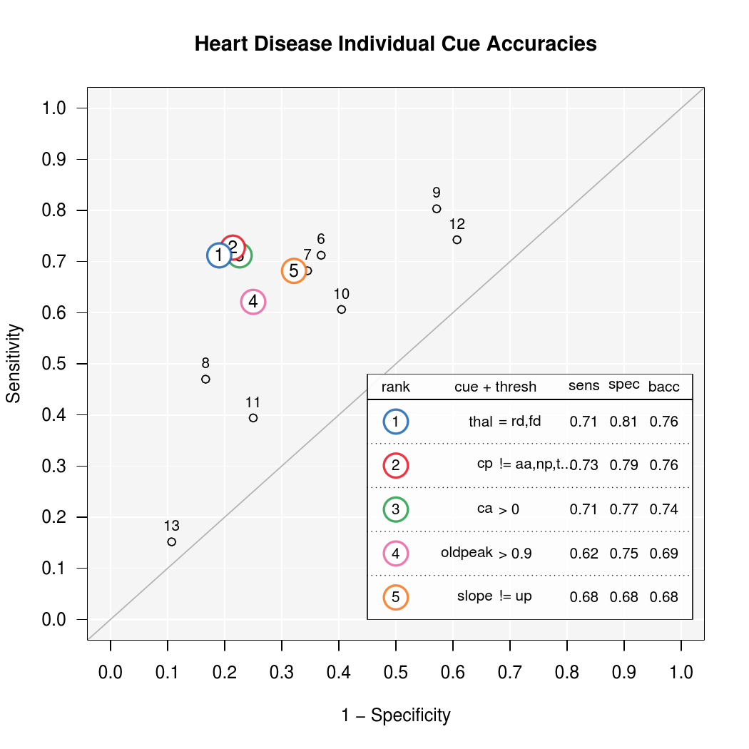
| Figure 7: Visualizing marginal (training) cue accuracies from the
heart.fft object by running plot(heart.fft, what =
‘‘cues’’, data = ‘‘train’’). Accuracy statistics are calculated
for each cue using the threshold that maximizes
bacc. Numbers indicate a cue’s ranked accuracy across all
cues in terms of bacc. The top five cues are colored and
described in the legend. All other cues in the data are shown as
black points. |
3.5 Additional options
The commands described so far cover the four basic steps in
constructing and evaluating FFTs with the FFTrees
package. Although these steps will be sufficient for many datasets and
applications, the package offers additional functions and options that
users might find helpful. We will now briefly describe five of the
additional functionalities and direct users to the documentation and
package guide (by evaluating FFTrees.guide()) for additional
options and examples.
3.5.1 Accessing additional outputs
An FFTrees object created with the FFTrees()
function contains several detailed outputs that can be accessed by
evaluating x$output, where x is an FFTrees
object created by the FFTrees() function, and output
is a named output of that object. To see all named outputs from an
FFTrees object, run names(x). Key outputs include:
x$cue.accuracies, which contains the decision thresholds and
marginal accuracies for each cue; x$decision, which contains
the classification decisions for all cases; x$levelout, which
indicates at which level in the FFT each case was classified; and
x$levelstats, which shows the cumulative classification
statistics for each level of the FFTs.
3.5.2 Predicting classes of new data
To make classification predictions for a new dataset using an
FFTrees object, use the predict(x, newdata)
function, where x is an FFTrees object, and
newdata is a data frame of new data. For example, one could
use the heart disease FFT (heart.fft) to predict the
diagnoses of a new set of patients whose cue information is stored in
a data frame called heart.new by running
predict(heart.fft, heart.new). This will return a vector of
classification predictions for each case in heart.new.
3.5.3 Defining an FFT in words
Some users might wish to implement a specific FFT to data, rather than
using an FFT construction algorithm to construct an optimized FFT. To
do this, users can verbally define a tree as a sentence by using the
my.tree argument when calling the FFTrees()
function. FFTrees will attempt to extract the cues, decision
thresholds, directions and exits from the sentence, and then apply the
FFT described to the specified data. For example, in the heart disease
data, one can directly define and implement a new heart disease FFT by
running the code: FFTrees(diagnosis ~ ., data =
heart.train, my.tree = ‘‘If chol > 350, predict True. If cp != {a}
predict False. If age <= 35, predict False. Otherwise, predict
True’’). Additional grammatical rules for verbally defining FFTs
are available in the package documentation.
3.5.4 Including cue costs
If the cues in a dataset have
specific and known implementation costs—like the financial cost of
a measurement, or the amount of time it takes to implement—they
can be included as a data frame in the cost.cues argument
when creating an FFTrees object. The cost.cues data
frame should have two columns: one specifying the name of a cue, and
one specifying the cost of that cue. The specific units used in
specifying costs (e.g., hours or $) are arbitrary, as long as they
are comparable across different cues. When cost.cues is
included, FFTrees will calculate the classification cost of
each case when applying an FFT to data. For example, in the heart disease data, each cue has a cost ranging
from a minimum of $1 (age) to $102.9 for the thallium
scintigraphy (thal) test.9 The costs are stored in the FFTrees package as a data frame
called heart.cost, with a column cue indicating the
names of the cues, and a column cost indicating their
costs. By including the argument cost.cues = heart.cost when
creating the heart disease FFT in Figure ??, one
can see in the summary output that using this FFT would cost
approximately $123 per patient on average. In contrast, using all
cues in classification would have cost approximately $300 per
patient, more than twice as much. Note that including cue costs does
not affect how trees are constructed. We will return
to the topic of incorporating cue costs in FFT construction in the
Discussion.
3.5.5 Creating a forest of FFTs
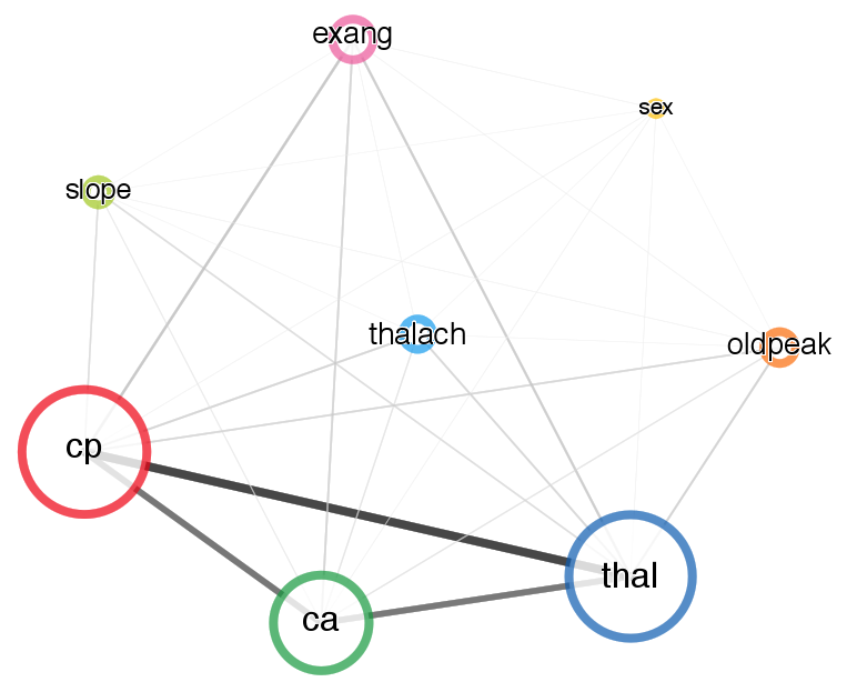
| Figure 8: Network plot of relationships between cues in the heart disease data created by plotting an FFForest object. The object represents a bootstrap simulation of 100 FFTs trained on different random subsets of the heart disease data. The size of a node reflects how often it occurs across different FFTs in the forest (i.e., its importance), while the weight of the connection between two nodes reflects how often they co-occur within individual FFTs. |
Additional insights into the role of cues in a dataset can be
gained by using the FFForest() function. This function
conducts a bootstrap simulation that applies the FFTrees()
function to random subsets of the data, thus creating a forest of many
FFTs, each constructed from different sets of cases.10
This forest of FFTs can be used to explore the importance of each cue
in a dataset, where cue importance is defined as the proportion of
FFTs in the forest for which a particular cue is selected. The more
often a cue is selected, the more important it is deemed to
be. Moreover, information about the co-occurrence of cues within FFTs
across the forest allows judging whether two cues tend to jointly
contribute to classification decisions within an FFT, or if they tend
to replace one another between FFTs.
Figure ?? shows the result of plotting the
result of FFForest() applied to the heart disease
data.11 This shows
that the three cues (thal, cp, ca) of the
FFT shown in Figure ?? were deemed the most
important (i.e., most commonly occurring) cues over the entire range
of FFTs (as indicated by their size) and were most likely to co-occur
(as indicated by the width of their connecting lines). This increases
our confidence that the three chosen cues are robust across a wide
range of subsets of the original data.
4 Prediction Simulation
FFTs are decision algorithms designed to provide simple rules of thumb
that can be easily understood and applied under cognitive and time
constraints, rather than solely maximizing decision
accuracy. That said, accuracy is certainly an important criterion in selecting a
decision algorithm. Moreover, while people might not be able to
implement complex algorithms “in the head”, they now often have easy
access to a computer or mobile phone that can quickly implement a
computationally intensive decision algorithm in negligible time. So
how well do FFTs predict data relative to more complex algorithms when
there are no computational restrictions? Prior research has suggested
that FFTs can predict data as well as algorithms such as logistic
regression and standard decision trees (Martignon et al., 2008; Woike,
Hoffrage & Hertwig, 2012; Woike et al., 2017). However, logistic
regression (in a non-regularised form) and standard decision trees
have strong competition from other algorithms. Support vector machines
(SVM) and random forests (RF, Kuhn & Johnson, 2013) are known to be
highly robust against overfitting and thus should provide a stronger
challenge to FFTs.
Thus, we are left with an important question: If computational
resources are no issue and we only care about prediction performance,
how good are FFTs created by the FFTrees package relative to
the benchmarks provided by complex compensatory algorithms? To answer
this question, we conducted a series of prediction simulations.
4.1 Simulation method
We obtained 10 real-world datasets from the UCI machine learning
repository (Lichman, 2013). A summary of the datasets is presented in
Table ??. The datasets differed in a variety of ways,
from their content domain, to the amount of cases (ranging from 68 to
17,895), to the number (from 6 to 280) and classes (numeric and
factor) of cues, to the base-rate of the criterion.
We implemented the prediction simulations using the benchmark
function in the mlr package (Bischl et al., 2016). Each
simulation proceeded as follows: The original dataset was split into a
50% training set for model fitting and a 50% testing set for
prediction. FFTs were constructed using four different algorithms:
ifan, dfan, max, and zig-zag. For both ifan and dfan, the maximum
number of levels was set to 4. As the max and zig-zag algorithms do
not specify size restrictions or pruning procedures (Martignon et al.,
2008), we did not restrict the size of FFTs created by either
algorithm. Model prediction performance was measured with balanced accuracy
(bacc) in the testing set. For simplicity, we do not consider
other accuracy measures such as weighted accuracy with sensitivity
weights other than 0.5, or overall accuracy, and do not claim that our
results will generalize to these or other accuracy measures. The speed
and frugality of the FFTs was measured by mcu and
pci.
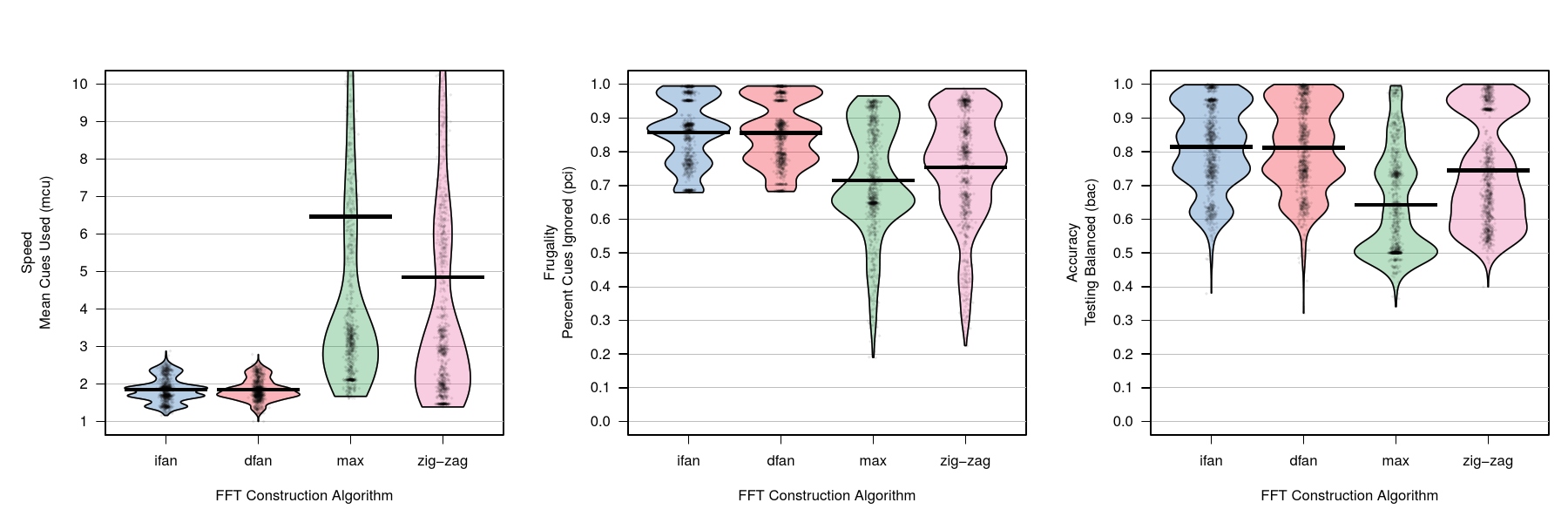
| Figure 9: Comparisons of the four different fast-and-frugal tree
construction algorithms collapsed across all simulations and
datasets. For the left panel (speed, measured by mean cues used,
mcu), lower values are better. For the middle and right
panels (measuring frugality by percent cues ignored, pci,
and balanced accuracy, bacc) higher values are
better. Horizontal lines in distributions represent means. Plots
were created using the yarrr package (Phillips, 2016). |
In addition to the four FFT construction algorithms, we performed
similar simulations for five competing decision algorithms: standard
decision trees (CART), using the rpart package (Therneau,
Atkinson & Ripley, 2015); logistic regression (LR), using the
stats package (R Core Team, 2016);12 regularised regression (RLR), using the
glmnet package (Friedman, Hastie & Tibshirani, 2010);
naïve Bayes (NB), using the e1071 package (Meyer,
Dimitriadou, Hornik, Weingessel & Leisch, 2015); random forests (RF),
using the randomForest package (Liaw & Wiener, 2002); and
support vector machines (SVM), also using the e1071 package
(Meyer et al., 2015). We used default parameter values for all of
these algorithms. We conducted 100 simulations for each dataset,
resulting in a total of 100 simulations for each model-data
combination. Complete simulation code and results are available on the
Open Science Framework at https://osf.io/m726x/ (Phillips et
al., 2017a).
4.2 Simulation results
We begin by comparing the four FFT construction algorithms, before
comparing the performance of FFTs to alternative prediction
algorithms.
4.2.1 Comparing FFT construction algorithms
The results for speed (mcu), frugality (pci), and
balanced accuracy (bacc) collapsed across all simulations and
testing datasets are presented in Figure ??. The
two fan algorithms had virtually identical performance in all
measures; therefore, we report their results simultaneously. With
respect to efficiency, the fan algorithms were faster13 and more
frugal than both max and zig-zag. Both fan algorithms had mean
mcu values of 1.85 (IQR = [1.65, 2.0]), whereas zig-zag had a
mean mcu value of 4.85 (IQR = [2.0, 6.2]), and max had a mean
mcu value of 6.5 (IQR = [2.6, 7.1]).14 Both fan algorithms were also
more accurate than max and zig-zag. The fan algorithms both had mean
bacc values of 0.81 (IQR = [0.73, 0.93]) compared to means of
0.64 (IQR = [0.50, 0.74]) and 0.75 (IQR = [0.61, 0.93]) for max and
zig-zag, respectively.
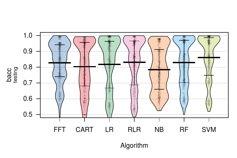
| Figure 10: Distributions of prediction performance, measured as balanced
accuracy (bacc) in testing across datasets. FFT results are
for FFTs built with the ifan construction algorithm. The SVM results
do not include data for the arrhythmia or audiology datasets due to
repeated crashing. Wide horizontal lines represent means and
vertical lines represent the 25th and 75th percentiles. Credible
intervals for means are not shown because they are virtually
identical to the sample means. Distributions for individual datasets
are presented in Figure ??. |
| Table 2: Dataset descriptions, FFT efficiency, and prediction accuracy measured in balanced accuracy (bacc) in the prediction simulations. All FFTs were constructed using the ifan algorithm. The efficiency measures apply only to FFTs. |
| Dataset | | | Efficiency1 | | | Prediction accuracy (bacc)2 |
|
Title | | Cases | | Cues | | Base rate | | | | mcu | | pci | | | | FFT | | CART | | LR | | RLR | | NB | | RF | | SVM |
| arrhythmia | | 68 | | 280 | | 0.29 | | | | 1.81 | | 0.99 | | | | 0.66 | | 0.64 | | 0.52 | | 0.70 | | 0.71 | | 0.69 | | —3 |
| audiology | | 226 | | 70 | | 0.10 | | | | 1.65 | | 0.98 | | | | 0.84 | | 0.65 | | 0.93 | | 0.85 | | 0.83 | | 0.72 | | —3 |
| breast | | 683 | | 10 | | 0.35 | | | | 1.42 | | 0.86 | | | | 0.94 | | 0.94 | | 0.96 | | 0.96 | | 0.97 | | 0.97 | | 0.97 |
| cmc | | 1,473 | | 10 | | 0.35 | | | | 2.20 | | 0.78 | | | | 0.61 | | 0.58 | | 0.56 | | 0.53 | | 0.59 | | 0.59 | | 0.57 |
| credit | | 666 | | 16 | | 0.45 | | | | 1.88 | | 0.88 | | | | 0.85 | | 0.85 | | 0.83 | | 0.87 | | 0.76 | | 0.87 | | 0.87 |
| dermatology | | 358 | | 35 | | 0.31 | | | | 1.69 | | 0.95 | | | | 0.99 | | 0.98 | | 0.99 | | 0.99 | | 0.69 | | 1.00 | | 1.00 |
| heart | | 303 | | 14 | | 0.46 | | | | 1.74 | | 0.88 | | | | 0.78 | | 0.76 | | 0.81 | | 0.82 | | 0.82 | | 0.81 | | 0.82 |
| occupancy | | 17,895 | | 6 | | 0.21 | | | | 1.89 | | 0.68 | | | | 0.96 | | 0.99 | | 0.99 | | 0.99 | | 0.98 | | 0.99 | | 0.99 |
| voting | | 435 | | 17 | | 0.61 | | | | 1.51 | | 0.91 | | | | 0.92 | | 0.96 | | 0.92 | | 0.96 | | 0.90 | | 0.96 | | 0.95 |
| yeast | | 1,484 | | 9 | | 0.16 | | | | 1.84 | | 0.80 | | | | 0.74 | | 0.69 | | 0.67 | | 0.64 | | 0.60 | | 0.70 | | 0.71 |
| Overall | | — | | — | | — | | | | 1.76 | | 0.87 | | | | 0.83 | | 0.80 | | 0.82 | | 0.83 | | 0.78 | | 0.83 | | 0.86† |
| 1 Efficiency measures only apply to FFTs:
mcu is mean cues used per case (speed), and
pci is percent of cues ignored (frugality). |
| 2 Prediction accuracy measures show mean balanced accuracy
(bacc) for six algorithms: FFT = fast-and-frugal trees using
the ifan construction algorithm, CART = standard decision trees, LR =
logistic regression, RLR = regularized logistic regression, NB =
naïve Bayes, RF = random forests, and SVM = support vector
machines. |
| 3 The SVM algorithm was unable to make predictions for both the arrhythmia or the audiology datasets due to repeated crashing. The overall accuracy prediction accuracy value for SVM thus only includes results from the other eight datasets.
|
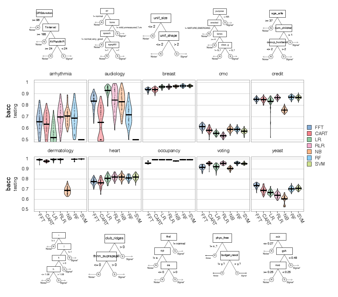
| Figure 11: Distributions of prediction balanced accuracy (bacc)
for each model and dataset in the prediction simulation. Horizontal
lines within plots represent means. FFT results are for FFTs built
with the ifan construction algorithm. The support vector machines
(SVM) algorithm could not make predictions in the arrhythmia and
audiology datasets due to repeated crashes. Next to each simulation
is a 100% training FFT produced by the ifan algorithm applied to
the full dataset. |
4.2.2 Comparing FFTs to other algorithms
We now compare the predictive accuracy of FFTs built with ifan to
alternative prediction algorithms. The mean prediction balanced
accuracy for each algorithm and dataset across all simulations are
presented in Table ?? and Figure
??. Results show that FFTs were competitive with other algorithms in
prediction performance. Collapsed across all datasets, the best
performing algorithm was support vector machines (SVM), with a mean
balanced accuracy of 0.86, followed closely by fast-and-frugal trees
(FFT), regularized logistic regression (RLR), and random forests (RF),
each with mean balanced accuracy scores of 0.83.15
Figure ?? shows the complete distribution of
prediction performance within each individual dataset as well as an
FFT constructed from the entire dataset.16 These results show that there was variability in the
rank order of algorithms across datasets, but FFTs were consistently
competitive in their prediction performance. Relative to other
algorithms, FFTs performed worst in the occupancy dataset, achieving a
mean balanced accuracy of .96, while most other algorithms
reached .99. In the cmc and yeast datasets, FFTs slightly outperformed
all other algorithms on average.
The 100% training FFTs in Figure ?? also
illustrate the diversity of FFTs created for different datasets. For
example, while some datasets such as breast and dermatology required
only small FFTs with a maximum of two cues, other datasets, such as
audiology, credit and bridges, produced larger FFTs that contained
four cues (the maximum allowed).
In addition to making accurate predictions, the FFTs created by
FFTrees were very efficient. Average mcu values,
representing how much information was necessary to make decisions,
were low, ranging from a minimum of 1.42 in the breast dataset, to a
maximum of 2.20 in the cmc dataset. Across all datasets, the mean
mcu value was 1.76, indicating that the FFTs required fewer
than two cues on average to make a fast classification decision. FFTs
were not just fast, they were also frugal. Mean pci values,
representing how much information the FFTs ignored, ranged from a
minimum of 68% in the occupancy dataset, to a maximum of 99% in the
arrhythmia dataset. Across all datasets, the mean pci value
was 87%, indicating that FFTs ignored 87% of all available
data. Together, these simulation results replicate and extend the
findings of others (Martignon et al., 2008; Woike et al., 2017):
Despite their simplicity and deliberate ignorance, FFTs can compete
with state-of-the-art decision algorithms in pure prediction
accuracy.
5 Discussion
FFTs are elegant, transparent and effective algorithms for making
binary classification decisions. Because they are predictive,
efficient and easy to implement, they have successfully been used in
many applied domains ranging from terrorism threat detection (Keller
& Katsikopoulos, 2016) to depression diagnosis (Jenny et al.,
2013). However, until now there has been no straightforward toolbox
for anyone to easily create FFTs from data. The FFTrees
package fills this gap. Importantly, our simulation results show that
FFTs, especially those constructed with the ifan algorithm, can be as
accurate as state-of-the-art classification algorithms. This
reinforces previous research showing that there is no inherent
trade-off between frugality and accuracy (Gigerenzer, Todd & the ABC
Research Group, 1999). Thus, users of the FFTrees package not
only can construct FFTs, but can use them with confidence for making
important predictions.
5.1 When and how should we use an FFT?
Although we have argued that FFTs are under-utilized, we also believe
that there are domains where an FFT is not the most appropriate
algorithm to use. To help decision makers decide whether to consider
FFTs or a alternative algorithm for making binary classification
decisions we recommend using the FFT presented in Figure
??. It answers the question “Should I consider an
FFT?” by considering four cues that matter when choosing a
classification algorithm: implementation, cost, transparency, and
prediction accuracy.
Implementation
Will the algorithm be implemented by a
person without a computational aid? If a decision needs to be implemented in real time by a human mind
without a computational aid then FFTs provide a functional and
accurate tool that can be quickly learned and easily used.
Costs
Are there substantial monetary or temporal costs
involved with implementing the decision? If it is costly to gather decision-relevant information, then FFTs are
particularly effective because they use so little information,
reducing costs in terms of money, time, and unnecessary tests
(Gigerenzer, 2015; Luan et al., 2011; Martignon et al., 2003). Consider the domain of medical decision making: Here, the speed and
frugality of effective FFTs are attractive because medical tests can
be expensive. As we have shown in the heart disease dataset, the FFT
in Figure ?? would have been almost 60% cheaper
to implement than an algorithm that uses all possible cues, with
perhaps no decrease in accuracy.
| Figure 12: An FFT to decide whether to consider an FFT or use an alternative algorithm for classifying cases for a decision task. The list of cues in this FFT are meant to be illustrative and not exhaustive. |
Transparency
Is it important to understand how the
algorithm works? Because an FFT can be explained either visually or verbally as a set
of simple rules, it is easy for decision makers to understand how an
FFT works and communicate it to others. By contrast, it is difficult
for anyone without extensive statistical training to understand and
implement more complex models like regression.
The transparency of FFTs not only makes them easier to understand,
use, and communicate, it also facilitates trouble-shooting when they
fail. As with a simple machine with only a few moving parts, it
should be relatively straightforward to see where and why an FFT might
be going wrong. For example, imagine a doctor making heart disease
diagnoses using the FFT presented in Figure
??. In her first year using the FFT, the tree
has a balanced accuracy of 90%, but in the following year, its
accuracy suddenly drops to 50%. What went wrong? Is one of the cues
in the tree no longer accurate? If so, which one? To find out, the
doctor could perform a few relatively simple checks. She could start
by first considering the first node: “If the thallium scintigraphy
test (thal) shows either a reversible defect (rd) or
a fixed defect (fd), predict high-risk.” To see if the
accuracy of classifications made by this cue has changed, she could
compare the classification of this node (i.e., those with reversible
or fixed defects) between years. If she finds that the accuracy rate
for patients classified at this node decreased from 85% to 40%, this
might suggest that the test is not being administered correctly, or
that her patient population has changed and that the test is less
accurate for this new population. On the other hand, if there was no
substantial change in accuracy for patients diagnosed at this node in
the FFT, she could be confident that the problem lies with a node
further down the tree.
In short, the simplicity and transparency of FFTs is not only
beneficial when the algorithm works well, but also allows decision
makers faced with a poorly performing tree to quickly diagnose why and
where it is failing. In contrast, detecting the cause(s) behind a
failing compensatory decision algorithm, which could hide behind a
variety of parameters, is considerably more difficult.
Prediction accuracy
Do FFTs reach similar (or better) prediction performance as other
algorithms in the problem domain? Like all decision algorithms, FFTs are neither inherently good nor bad
at prediction (Gigerenzer, Todd & the ABC Research Group,
1999). Rather, their performance depends on their match to the task
environment, and the demands of the decision maker. Indeed, there is
“no free lunch” in classification tasks, meaning that no single
learning algorithm is better a priori than any other when
facing an unknown dataset (Wolpert, 1996). Our simulations across 10
diverse datasets have shown that FFTs can compete with complex
machine learning algorithms in data prediction alone, they do not
prove that FFTs always will.
This raises an important question: When can we expect that FFTs will
perform well and when can we expect that they will not? While a
complete answer to this question is beyond the scope of this paper, we
can point to one general class of datasets for which FFTs will not
predict data as well as compensatory algorithms: namely, those with
many cues that each are weakly predictive of the criterion, but where
a function of the cues (i.e., a weighted linear combination) is highly
predictive. For example, one could generate a dataset
containing 10 cues X1, X2, …, X10, with a binary,
Bernoulli-distributed criterion y and a probability of success
defined by
logit(1 · X1 + 1 · X2 + 1 · X3 + … + 1
· X10). An FFT would tend to make poor predictions for this
data as each individual cue is not very predictive of the
criterion. By contrast, a logistic regression model with a
sufficiently large training dataset could make accurate predictions
for these data because the sum of all cues, which a regression
equation can easily capture, is highly predictive of the criterion.
However, if we allow for some cues to be more predictive than others,
then FFTs can make good predictions even when the true generative
model is a linear weighed combination of the cues. For example,
if the probability of success was defined as a weighted
sum of the cues with highly skewed weights, such as
logit(100 · X1 + 50 · X2 + 25 · X3 + … + 1
· X10), an FFT could perform quite well by focusing on
a few highly predictive cues (i.e., X1, X2, and X3),
and ignoring the rest.
Ultimately, the question which algorithm yields the best predictive
performance for a dataset is an empirical, rather than an
ideological question. While it is helpful to understand which
properties of data generally affect the relative performance of
different decision algorithms, one should be cautious in discarding
an algorithm a priori, without actually evaluating its
prediction (rather than fitting) performance for a dataset. When
viewing prediction algorithms as tools, whose function partly depends
on their fit to the features of specific datasets, even algorithms
that, by all logic “should” fail can be surprisingly successful.
5.2 Future directions
The FFTrees package is a growing toolbox for creating,
customizing, and applying fast-and-frugal trees. As such, the FFT
construction algorithms, metrics, and visualizations currently
included in FFTrees provide just a starting point rather than
a final product. Although we have ideas and plans for extensions, the
goals and directions of future versions will also depend on the
feedback from users, inputs from developers, and needs of
practitioners. We now identify three key areas for further developing
FFTrees.
5.2.1 Incorporating cue costs in FFT construction
In decision tasks such as medial diagnoses, information can come at
significant costs in terms of time, money, or other factors, such as
physical and psychological stress. As we have described, FFTs are
almost inherently cheap to use as they typically require very little
information to make a decision. However, this does not mean that all
FFTs are equally cost efficient—one FFT might be much cheaper to
use than another, either because it uses less expensive cues, or
because it uses them in a more cost efficient order. While
FFTrees can calculate classification costs when applying FFTs
to data (when the user specifies cue costs using the
cost.cues argument) these costs are not currently used during
FFT construction. When cue costs are ignored, an FFT construction
algorithm might construct trees containing cues that are relatively
expensive to use, but miss slightly less accurate trees that would be
much cheaper to implement. For instance, in the heart disease dataset,
FFTrees puts a relatively expensive cue (thal:
$102.90) at the first node of the FFT, and a very cheap cue
(cp: $1) at the second node. However, inspecting the cue
accuracies in Figure ?? shows that the cues have
comparable accuracies. Thus, we would expect that simply changing the
order of these cues could substantially reduce the cost of applying
the FFT with very little reduction in decision
accuracy. As the ifan construction algorithm ignored cue costs, it
returned a relatively expensive FFT and missed a much cheaper variant
that may yield a similar accuracy. The issue of considering
explicit costs for test construction has been discussed in
the medical decision making literature (e.g., Hershey, Cebul &
Williams, 1986), and costs have been incorporated into standard decision
tree construction algorithms (Lomax & Vadera, 2013). One major
feature of a future FFTrees toolbox would be to allow
users to specify the cost of obtaining values from each cue, and
then incorporate both cue costs and decision accuracy in constructing
FFTs.
5.2.2 Detecting and adapting to performance changes
Many decision tasks occur in dynamic environments, where conditions
are not static, but can change over time. Terrorists can change how
they approach military checkpoints (Keller & Katsikopoulos, 2016),
financial institutions can vary their investment strategies (Aikman et
al., 2014), and new patient populations can enter emergency rooms
(Trzeciak & Rivers, 2003). In decision tasks where FFTs are applied
to potentially dynamic data, a change detection algorithm such as
those used in image processing (e.g., Radke, Andra, Al-Kofahi &
Roysam, 2005) and time series (e.g., Kim, 2000; Ray & Tsay, 2002)
could be useful in tracking changes in the performance of an FFT over
time as it is applied to new batches of data (see Todd & Dieckmann,
2004, for a similar discussion). Consider how a change detection
algorithm could improve doctors’ use of the heart disease FFT. Given
historical training data, a change detection algorithm could maintain
a series of expected probabilities that future patients will be
classified at each exit branch in the tree, as well as the probability
of classification success at each branch. For example, the algorithm
might predict that 50% of future patients should be classified at the
first node of the tree, and of those patients, 75% should be
correctly classified. As new patients are classified using the tree
over time, the algorithm could compare the classification rates of new
patients to its expectations from historical data. If the algorithm
determines that the new classification rates are substantially
different from what was expected, FFTrees could notify the
user that a meaningful change may have occurred. This could spur the
user to re-evaluate how well specific cue values are being measured
(i.e., a malfunctioning medical test) or to consider constructing a
new FFT trained on more recent data.
5.2.3 Modeling behavioral data
In this paper, we have focused on using FFTs to predict matters of
fact or objective states (like patients with high vs. low risks for
heart disease). However, FFTrees could also be used to model
behavioral data with binary outcomes (like doctors’ decisions based on
classifying patients). Both fast-and-frugal and standard decision
trees have successfully been used to model decision making processes
in memory (Batchelder & Riefer, 1990) and quantitative judgments
(Gigerenzer & Goldstein, 1999; Gigerenzer, Todd & the ABC Research
Group, 1999; Rieskamp & Hoffrage, 1999). Software packages such as
multiTree (Moshagen, 2010) exist that automate the modeling
process. FFTrees could also in principle be used to model
individual-level decision processes. While we support such efforts, we also caution against a naive
interpretation of FFTs as process models without a modicum of
skepticism and additional supporting evidence. When applied to
behavioral data, the FFT construction algorithms in FFTrees
will prefer cues that predict the criterion value without any
consideration of their their psychological plausibility. An FFT could
rank cues in an order that makes no psychological sense, or might
select cues that were not even encoded by the decision maker. While a
good fit—or better, successful prediction—of some statistical
model may be necessary to be considered as a process model, it is not
sufficient. A convincing case for FFTs as process models should
include process predictions (Johnson, Schulte-Mecklenbeck &
Willemsen, 2008), such as increasing response latencies corresponding
to lower levels of a tree (see Fific, Little & Nosofsky, 2010, for a
a related example), and a conceptual scope of the decision making
process (Jarecki, Tan & Jenny, 2016).
6 Conclusion
The purpose of this article is to highlight the effectiveness of
fast-and-frugal trees, and to make them accessible to interested users
via FFTrees. By focusing on the creation and evaluation of
FFTs, we have been silent about how they are or should be used. For
instance, FFTs can model someone’s judgment or some objective state or
fact, and can be interpreted in both a descriptive or a normative
fashion. Irrespective of one’s stance in this debate, an FFT is designed to
provide accurate and robust predictions at low costs. If it achieves
this goal, its transparency provides a suggestion for revising our
beliefs about the causal texture of a particular task or domain. Thus,
while it would seem inflated to view any successful FFT as a process
model or theory, it could certainly serve as a tool to inform our
theorizing.
Realizing that simple FFTs can be as accurate as far more complex
models raises new issues regarding their acceptance and
justification. Even if skeptics were persuaded that frugality does not always
decrease accuracy it will remain a challenge how ignoring information
can be justified when errors occur. Imagine a doctor making a
frugal classification decision that proves to be wrong. Can she really
claim with authority and confidence that it was legitimate and in the
patient’s best interest to ignore most of the available information? Given our results, there is no a priori reason to believe that
a more comprehensive or complex algorithm would have been less
error-prone than an FFT. Nevertheless, it is clear that a society or
institution that primarily aims to assign blame, rather than learn
from errors, may be reluctant to adopt fast-and-frugal algorithms.
At the same time, practical concerns and persistent pressures to
reduce costs push decision makers towards more frugal models. Just as
ignoring information may be hard to justify, it is difficult to insist
on using irrelevant information that provides no benefit in predictive
accuracy. Thus, answering the question if and how FFTs should be used
touches upon many issues of public policy and of legal or moral
responsibility. Whenever making predictions for important tasks, we
ultimately strive for an acceptable balance between accuracy and
frugality. The FFTrees package helps us to find, measure, and
better understand this balance.
References
Aikman, D., Galesic, M., Gigerenzer, G., Kapadia, S., Katsikopoulos, K., Kothiyal, A., . . . Neumann, T. (2014). Taking uncertainty seriously: Simplicity versus complexity in financial regulation (Tech. Rep.). London, UK: Bank of England Financial Stability Paper, 28.
Akane, O., & Shane, S. (2017, Feb 23). Think a negative tweet from Trump crushes a stock? Think again. The Wall Street Journal. Retrieved from http://www.wsj.com/graphics/trump-market-tweets/
Batchelder, W. H., & Riefer, D. M. (1990). Multinomial processing models of source monitoring. Psychological Review, 97(4), 548–564.
Bischl, B., Lang, M., Kotthoff, L., Schiffner, J., Richter, J., Jones, Z., & Casalicchio, G. (2016). mlr: Machine learning in R [Computer software manual]. Retrieved from https://CRAN.R-project.org/package=mlr.
Breiman, L., Friedman, J. H., Olshen, R. A., & Stone, C. J. (1984). Classification and regression trees. Belmont, CA: Wadsworth.
Dawes, R. M. (1979). The robust beauty of improper linear models in decision making. American Psychologist, 34(7), 571–582.
Detrano, R., Janosi, A., Steinbrunn, W., Pfisterer, M., Schmid, J.-J., Sandhu, S., . . . Froelicher, V. (1989). International application of a new probability algorithm for the diagnosis of coronary artery disease. The American Journal of Cardiology, 64(5), 304–310.
Dhami, M. K. (2003). Psychological models of professional decision making. Psychological Science, 14(2), 175–180.
Dhami, M. K., & Ayton, P. (2001). Bailing and jailing the fast and frugal way. Journal of Behavioral Decision Making, 14(2), 141–168.
Dhami, M. K., & Harries, C. (2001). Fast and frugal versus regression models of human judgement. Thinking & Reasoning, 7(1), 5–27.
Einhorn, H. J., & Hogarth, R. M. (1975). Unit weighting schemes for decision making. Organizational Behavior and Human Performance, 13(2), 171–192.
Fific, M., Little, D. R., & Nosofsky, R. M. (2010). Logical-rule models of classification response times: A synthesis of mental-architecture, random-walk, and decision-bound approaches. Psychological Review, 117(2), 309–348.
Fischer, J. E., Steiner, F., Zucol, F., Berger, C., Martignon, L., Bossart, W., . . . Nadal, D. (2002). Use of simple heuristics to target macrolide prescription in children with community-acquired pneumonia. Archives of Pediatrics & Adolescent Medicine, 156(10), 1005-1008.
Friedman, J., Hastie, T., & Tibshirani, R. (2010). Regularization paths for generalized linear models via coordinate descent. Journal of Statistical Software, 33(1), 1–22.
Galesic, M., Garcia-Retamero, R., & Gigerenzer, G. (2009). Using icon arrays to communicate medical risks: Overcoming low numeracy. Health Psychology, 28(2), 210.
Gigerenzer, G. (2015). Calculated risks: How to know when numbers deceive you. New York, NY: Simon and Schuster.
Gigerenzer, G., & Brighton, H. (2009). Homo heuristicus: Why biased minds make better inferences. Topics in Cognitive Science, 1(1), 107–143.
Gigerenzer, G., Czerlinski, J., & Martignon, L. (1999). How good are fast and frugal heuristics? In J. Shanteau, B. Mellers, & D. Schum (Eds.), Decision science and technology (pp. 81–103). New York, NY: Springer.
Gigerenzer, G., & Gaissmaier, W. (2011). Heuristic decision making. Annual Review of Psychology, 62, 451–482.
Gigerenzer, G., & Goldstein, D. G. (1996). Reasoning the fast and frugal way: Models of bounded rationality. Psychological Review, 103(4), 650–669.
Gigerenzer, G., & Goldstein, D. G. (1999). Betting on one good reason: The take the best heuristic. In Simple heuristics that make us smart (pp. 75–95). New York, NY: Oxford University Press.
Gigerenzer, G., Todd, P. M., & the ABC Research Group. (1999). Simple heuristics that make us smart. New York, NY: Oxford University Press.
Green, D. M., & Swets, J. A. (1966). Signal detection theory and psychophysics (Vol. 1). New York, NY: Wiley.
Green, L., & Mehr, D. (1997). What alters physicians’ decisions to admit to the coronary care unit? Journal of Family Practice, 45(3), 219–226.
Hammond, K. R. (1955). Probabilistic functioning and the clinical method. Psychological Review, 62(4), 255–262.
Hershey, J. C., Cebul, R. D., & Williams, S. V. (1986). Clinical guidelines for using two dichotomous tests. Medical Decision Making, 6(2), 68–78.
James, G., Witten, D., Hastie, T., & Tibshirani, R. (2013). An introduction to statistical learning (Vol. 6). New York, NY: Springer.
Jarecki, J. B., Tan, J. H., & Jenny, M. A. (2017). What is a cognitive process model? A disambiguation. Unpublished manuscript, Department of Economic Psychology, University of Basel.
Jenny, M. A., Pachur, T., Williams, S. L., Becker, E., & Margraf, J. (2013). Simple rules for detecting depression. Journal of Applied Research in Memory and Cognition, 2(3), 149–157.
Johnson, E. J., Schulte-Mecklenbeck, M., & Willemsen, M. C. (2008). Process models deserve process data: Comment on Brandstätter, Gigerenzer, and Hertwig (2006). Psychological Review, 115(1), 263–73.
Keller, N., & Katsikopoulos, K. V. (2016). On the role of psychological heuristics in operational research; and a demonstration in military stability operations. European Journal of Operational Research, 249(3), 1063–1073.
Kim, J.-Y. (2000). Detection of change in persistence of a linear time series. Journal of Econometrics, 95(1), 97–116.
Kuhn, M., & Johnson, K. (2013). Applied predictive modeling. New York, NY: Springer.
Liaw, A., & Wiener, M. (2002). Classification and regression by randomforest. R News, 2(3), 18–22. Retrieved from http://CRAN.R-project.org/doc/Rnews/
Lichman, M. (2013). UCI machine learning repository. Retrieved from http://archive.ics.uci.edu/ml
Lomax, S., & Vadera, S. (2013). A survey of cost-sensitive decision tree induction algorithms. ACM Computing Surveys (CSUR), 45(2), 16.
Luan, S., & Reb, J. (2017). Fast-and-frugal trees as noncompensatory models of performance-based personnel decisions. Organizational Behavior and Human Decision Processes, 141, 29–42.
Luan, S., Schooler, L. J., & Gigerenzer, G. (2011). A signal-detection analysis of fast-and-frugal trees. Psychological Review, 118(2), 316–338
Macmillan, N. A., & Creelman, C. D. (2005). Detection theory: A user’s guide (2nd ed.). Mahwah, NJ: Lawrence Erlbaum.
Martignon, L., & Hoffrage, U. (2002). Fast, frugal, and fit: Simple heuristics for paired comparison. Theory and Decision, 52(1), 29–71.
Martignon, L., Katsikopoulos, K. V., & Woike, J. K. (2008). Categorization with limited resources: A family of simple heuristics. Journal of Mathematical Psychology, 52(6), 352–361.
Martignon, L., Vitouch, O., Takezawa, M., & Forster, M. R. (2003). Naive and yet enlightened: From natural frequencies to fast and frugal decision trees. In L. M. D. Hardman (Eds.), Thinking: Psychological perspectives on reasoning, judgment, and decision making (pp. 189–211). Chichester, UK: Wiley.
Meehl, P. E. (1954). Clinical versus statistical prediction: A theoretical analysis and a review of the evidence. Minneapolis, MN: University of Minnesota Press.
Meyer, D., Dimitriadou, E., Hornik, K., Weingessel, A., & Leisch, F. (2015). e1071: Misc functions of the department of statistics, probability theory group (formerly: E1071), tu wien [Computer software manual]. Retrieved from https://CRAN.R-project.org/package=e1071.
Moshagen, M. (2010). multiTree: A computer program for the analysis of multinomial processing tree models. Behavior Research Methods, 42(1), 42–54.
Neth, H., & Gigerenzer, G. (2015). Heuristics: Tools for an uncertain world. In R. Scott & S. Kosslyn (Eds.), Emerging trends in the social and behavioral sciences. New York, NY: Wiley.
Newell, B. R., Rakow, T., Weston, N. J., & Shanks, D. R. (2004). Search strategies in decision making: The success of “success”. Journal of Behavioral Decision Making, 17(2), 117–137.
Phillips, N. D. (2016). yarrr: A companion to the e-book YaRrr!: The Pirate’s Guide to R [Computer software manual]. Retrieved from https://CRAN.R-project.org/package=yarrr.
Phillips, N. D., Neth, H., Woike, J. K., & Gaissmaier, W. (2017a, Jun). FFTrees: A toolbox to create, visualize and evaluate fast-and-frugal decision trees. Open Science Framework. Retrieved from osf.io/m726x
Phillips, N. D., Neth, H., Woike, J. K., & Gaissmaier, W. (2017b). FFTrees: Generate, visualize, and compare fast and frugal decision trees [Computer software manual]. Retrieved from https://CRAN.R-project.org/package=FFTrees.
Pitt, M. A., & Myung, I. J. (2002). When a good fit can be bad. Trends in Cognitive Sciences, 6(10), 421–425.
Quinlan, J. R. (1986). Induction of decision trees. Machine Learning, 1(1), 81–106.
Quinlan, J. R. (1987). Simplifying decision trees. International Journal of Man-Machine Studies, 27(3), 221–234.
Quinlan, J. R. (1993). C4.5: Programs for machine learning. San Mateo, CA: Morgan Kaufmann.
R Core Team. (2016). R: A language and environment for statistical computing [Computer software manual]. Vienna, Austria. Retrieved from https://www.R-project.org
Radke, R. J., Andra, S., Al-Kofahi, O., & Roysam, B. (2005). Image change detection algorithms: A systematic survey. IEEE transactions on image processing, 14(3), 294–307.
Ray, B. K., & Tsay, R. S. (2002). Bayesian methods for change-point detection in long-range dependent processes. Journal of Time Series Analysis, 23(6), 687–705.
Rieskamp, J., & Hoffrage, U. (1999). When do people use simple heuristics and how can we tell? In G. Gigerenzer, P. Todd, & the ABC Research Group (Eds.), Simple heuristics that make us smart (pp. 141–167). New York: Oxford University Press.
Roberts, S., & Pashler, H. (2000). How persuasive is a good fit? A comment on theory testing. Psychological Review, 107(2), 358–367.
Silver, N. (2012). The signal and the noise: Why so many predictions fail, but some don’t. London, UK: Allen Lane.
Super, G. (1984). START: A triage training module. Newport Beach, CA: Hoag Memorial Hospital Presbyterian.
Therneau, T., Atkinson, B., & Ripley, B. (2015). rpart: Recursive partitioning and regression trees [Computer software manual]. Retrieved from https://CRAN.R-project.org/package=rpart.
Todd, P. M., & Dieckmann, A. (2005). Heuristics for ordering cue-search in decision making. In L. K. Saul , Y. Weiss, & L. Bottou (Eds.), Advances in neural information processing systems (Vol. 17, pp. 1393–1400). Cambridge, MA: MIT
Press.
Trzeciak, S., & Rivers, E. (2003). Emergency department overcrowding in the United States: An emerging threat to patient safety and public health. Emergency Medicine Journal, 20(5), 402–405.
Walsh, M. M., Einstein, E. H., & Gluck, K. A. (2013). A quantification of robustness. Journal of Applied Research in Memory and Cognition, 2(3), 137–148.
Wegwarth, O., Gaissmaier, W., & Gigerenzer, G. (2009). Smart strategies for doctors and doctors-in-training: Heuristics in medicine. Medical Education, 43(8), 721–728.
Woike, J. K., Hoffrage, U., & Hertwig, R. (2012). Estimating quantities: Comparing simple heuristics and machine learning algorithms. In A. E. P. Villa et al. (Eds.), International Conference on Artificial Neural Networks (pp. 483–490). Heidelberg: Springer.
Woike, J. K., Hoffrage, U., & Martignon, L. (2017). Integrating and testing natural frequencies naïve Bayes, and fast and frugal trees. Decision. (Advance online publication)
Woike, J. K., Hoffrage, U., & Petty, J. S. (2015). Picking profitable investments: The success of equal weighting in simulated venture capitalist decision making. Journal of Business Research, 68(8), 1705–1716.
Wolpert, D. H. (1996). The existence of a priori distinctions between learning algorithms. Neural Computation, 8(7), 1391–1420.
Appendix
6.1 FFT fan construction algorithms
The following are descriptions of the fan FFT construction algorithms, ifan and dfan as implemented in FFTrees version 1.3.2. Our terminology is as follows:
- Criterion:
- Y is a binary vector of length M indicating the true criterion value (True or False) for all cases.
- Cue Matrix:
- Z is an M · N matrix (or in R terms, a data frame) of cues (predictors), containing M rows (cases) and N columns (cues).
- Cues:
- Xi, i ∈ 1, 2, … N are N cue vectors of length M, where some vectors are nominal factors, and others are on a numeric (either continuous or discrete) scale.
- Decision threshold and decision direction:
- Ti is a decision threshold, and Di is a decision direction for the i-th cue that jointly map cue values to positive (i.e., criterion = True or 1) decisions. For numeric cues, Ti is a number and Di a direction Di ∈ {>, < }. For example, for a numeric cue age, the threshold and direction combination age > 30, where T = 30 and D = >, means that age values greater than 30 are predicted to have positive criterion values, while age values less than or equal to 30 are predicted to have negative (i.e., criterion = False or 0) criterion values. For factor cues, Ti is a set of factor values and Di ∈ {∈, ∉ } For example, color ∈ {blue, green} has a decision threshold T = {blue, green} and decision direction D = ∈, meaning that colors equal to blue or green are predicted to have positive criterion values, and colors not equal to blue or green (∉) are predicted to have negative criterion values.
6.2 Fan algorithm parameters
Both fan algorithms have the following five parameters:
- goal.chase:
- A statistic that is maximized when calculating cue thresholds and ranking cues.
Default: goal.chase = bacc.
- goal:
- A statistic that is maximized when selecting a final FFT from an existing set of FFTs. Default: goal = wacc.
- max.levels:
- The maximum number of levels allowed in an FFT.
Default: max.levels = 4.
- max.numcat:
- The number of (equally spaced) numeric thresholds compared when calculating thresholds for numeric cues.
Default: max.numcat = 20.
- stopping.par:
- The minimum percentage of training data required by each node.
Default: stopping.par = .10.
6.3 The ifan algorithm
The ifan algorithm assumes independence between cues and is defined as follows:
- Calculate decision thresholds and directions for each cue: For each cue Xi, calculate a decision threshold Ti and decision direction Di that maximizes goal.chase when the decisions made by this cue (and ignoring all other cues) are compared to the true criterion values for all M cases. In version 1.3.0 of FFTrees, this is done in a brute-force fashion and comprises several sub-steps that distinguish between numeric and factor cues:
- For numeric cues, test max.numcat · 2 different thresholds and direction pairs by combining all possible combinations of max.numcat (with a default value of 20) decision thresholds (equally spaced numeric values ranging from the minimum to the maximum cue value) with 2 decision directions (> and <). Select the threshold-direction pair with the highest goal.chase value.
- For factor cues, the exit direction for each factor level is determined in a two-step procedure:
- Calculate the goal.chase of all possible combinations of individual factor levels and decision directions (∈ and ∉). For example, given a cue color with three possible values red, green and blue, test six combinations of decision thresholds and directions: color ∈ red, color ∉ red, color ∈ green, color ∉ green, color ∈ blue, color ∉ blue.
- For each factor level, remove the decision direction with the lower goal.chase value from the set. For example, if color ∈ red has a balanced accuracy of 0.75, and color ∉ red has a balanced accuracy of 0.45, then remove the combination color ∉ red.
- For each decision direction, rank cue thresholds in order of goal.chase. For example, considering the ∈ direction, the color thresholds could be ranked as color ∈ red = 0.75, color ∈ green = 0.6 (here, we assume that the color ∈ blue threshold was removed because the threshold color ∉ blue had a higher value of goal.chase).
- Determine a candidate set of cue thresholds by sequentially combining individual thresholds in order of rank, starting with the highest ranked threshold. As each additional threshold is added to the set, re-calculate the goal.chase of the set. Continue adding factor values to the set as long as goal.chase increases. As soon as goal.chase decreases with an additional factor value, stop the process and use the previously defined threshold set. Complete this process for both the ∈ and the ∉ decision directions, resulting in two candidate sets of factor values (one for the ∈ direction and one for the ∉ direction).
- Compare the goal.chase values of the final two sets of factor values and select the set with the higher goal.chase value as the final decision threshold, with a corresponding decision direction.
- Rank order cues by goal.chase: Rank order cues (combined with their corresponding decision thresholds and directions calculated in Step 1) by their goal.chase values. Select the top max.levels cues and discard the rest.
- Create a fan of several FFTs: Create 2max.levels − 1 FFTs {F1, F2, … , F2max.levels − 1} by placing the cues selected and ordered in Step 2 in sequential nodes, using all possible FFT exit structures, where nodes 1 through max.levels − 1 can have either a positive or a negative exit, and the final max.levels node has both a positive and negative exit.
- Prune FFTs: For each tree Fi, classify all cases. If any lower nodes in the tree contain fewer than stopping.par percent of all cases, remove those nodes and force the final remaining (lowest) node in the tree to have both a positive and negative exit.
- Select FFT with highest goal: Calculate the goal value of each tree. Select the tree with the highest goal value as the final tree.
6.4 The dfan algorithm
The dfan algorithm assumes dependencies (or interactions)
between cues and is defined as follows:
- Create FFTs with different exit structures: Given max.levels, create 2max.levels − 1 FFTs {F1, F2, … F2max.levels − 1} by using all possible FFT exit structures, where nodes 1 through max.levels − 1 can have either a positive or a negative exit, and the final (max.levels.) node has both a positive and a negative exit. For example, if max.levels = 3, then four FFT skeletons are created: FFT #1 = {0, 0, .5}, FFT #2 = {0, 1, .5}, FFT #3 = {1, 0, .5}, FFT #4 = {1, 1, .5}, where 0, 1, and .5 represent negative exits, positive exits, and both negative and positive exits, respectively.
- Create new decision thresholds, rank cues, and select top ranked cue for next empty level: Calculate decision thresholds, and directions for all cues using the procedure outlined in Step 1 of the ifan algorithm. Rank order cues by their goal.chase values. Select the top ranked cue and assign to the current node.
- Classify cases in current node: Make classification decisions for cases that satisfy the decision criteria for the current node.
- Repeat Steps 2 and 3: Recursively repeat Steps 2 and 3, calculating new decision thresholds and directions for each cue based on cases not yet classified by earlier nodes, and assigning the cue with the highest goal.chase to the next empty node. Repeat until all cases are classified.
- Prune FFTs: See ifan Step 4 (above).
- Select FFT with highest goal: See ifan Step 5 (above).
This document was translated from LATEX by
HEVEA.