Judgment and Decision Making, Vol. 13, No. 4, July 2018, pp. 309-321

Predictions of magnitudes (costs, durations, environmental events) are often given as uncertainty intervals (ranges). When are such forecasts judged to be correct? We report results of four experiments showing that forecasted ranges of expected natural events (floods and volcanic eruptions) are perceived as accurate when an observed magnitude falls inside or at the boundary of the range, with little regard to its position relative to the “most likely” (central) estimate. All outcomes that fell inside a wide interval were perceived as equally well captured by the forecast, whereas identical outcomes falling outside a narrow range were deemed to be incorrectly predicted, in proportion to the magnitude of deviation. In these studies, ranges function as categories, with boundaries distinguishing between right or wrong predictions, even for outcome distributions that are acknowledged as continuous, and for boundaries that are arbitrarily defined (for instance, when the narrow prediction interval is defined as capturing 50 percent and the wide 90 percent of all potential outcomes). However, the boundary effect is affected by label. When the upper limit of a range is described as a value that “can” occur (Experiment 5), outcomes both below and beyond this value were regarded as consistent with the forecast.

Keywords: prediction, forecasting, prediction intervals

1  Introduction

Most prediction tasks are surrounded by uncertainty. Degree of uncertainty can be incorporated in forecasts in various ways: by verbal hedges or phrases conveying likelihood (it is likely that the sea level will increase by 60 cm), by numerical probabilities (there is a 70% chance of such an increase), or by prediction intervals bounded by maximum and minimum values (the sea level will increase by 50–80 cm). Such ranges are often combined with probabilities to form, for instance, 95% uncertainty intervals, or can be accompanied by figures showing the entire distribution (Dieckman, Peters, Gregory & Tusler, 2012).

A vast research literature in judgmental forecasting has scrutinized the accuracy of such forecasts, what they are intended to mean, and how they are perceived by recipients. For instance, verbal phrases are vague in terms of the probabilities they convey (Budescu & Wallsten, 1995), but unequivocal in selectively directing the listener’s attention towards the occurrence or non-occurrence of the target event, in other words they are “directional” and can be classified as either positive or negative (Honda & Yamagishi, 2017; Teigen & Brun, 1995). Numeric probabilities are often overestimated (Moore & Healy, 2008; Riege & Teigen, 2017), whereas uncertainty intervals are typically too narrow (Moore, Tenney & Haran, 2016; Teigen & Jørgensen, 2005). Much less is known about how forecasts are evaluated after the actual outcomes have occurred. For instance, a meteorologist says that El Niño has “a 60% chance” of occurring later in the season. How correct is this forecast if El Niño actually occurs? Perhaps we feel that the forecaster was on the right track, by suggesting a chance above even, but a bit too low. Another forecaster in the same situation might prefer to say that El Niño has “at least a 50% chance” of occurring. Even though this is a less precise forecast, it implies a positive expectation (perhaps suggesting an increasing trend) and could be considered by some listeners as better than an exact 60% estimate (Hohle & Teigen, 2018). A third forecaster who says, more cautiously, that El Niño is “not certain” to occur, may also have a 60% probability in mind, but appears less accurate than the other two because of the negative directionality inherent in the phrase “not certain” (Teigen, 1988).

The research reported in the present paper examines how people evaluate interval (range) predictions, and specifically the role of the lower and upper bounds of such intervals for post hoc accuracy judgments. We assume that an interval forecast of tomorrow’s temperature of 11–15 ^∘C will be regarded as more accurate if the temperature reaches 14 or 15 ^∘C than if it climbs to 17 or 19 ^∘C. Does it become even more accurate if the temperature stays closer to the center of the uncertainty interval? Is, for instance, a temperature of 13 or 14 ^∘C more accurately predicted by the interval than one of 15 ^∘C? Will all deviations from the expected, “most likely” estimate be considered wrong in proportion to the magnitude of this deviation, or are deviations falling outside of the interval judged as qualitatively different from deviations falling inside he interval? If such is the case (as we think it is), will a forecaster be perceived as more correct by simply widening the prediction interval to 8–17 ^∘C?

Wide range estimates might be less informative (Yaniv & Foster, 1995) and reveal more uncertainty (Løhre & Teigen, 2017) than narrow ranges at the time when they are issued, but may in retrospect appear as better forecasts, by their ability to account for a large variety of outcomes. All values inside an uncertainty interval are in a sense anticipated, by belonging to the set of predicted outcomes. Dieckman, Peters and Gregory (2015) found that some people regard all alternatives inside an uncertainty interval as equally probable. This would reinforce a tendency to think that even outcomes near the interval bounds have been “accurately” predicted, on par with other outcomes in the distribution. But, even without assumptions of a flat distribution, we suspect that outcomes within the uncertainty intervals (including those at the upper and lower interval bounds) will be viewed as accurately predicted, in contrast to outcomes falling above the upper limit or below the lower limit of an estimated range. We explore in the present studies the nature and extent of this boundary effect in range forecasts. The studies were designed to test the following hypotheses:

1. Outcomes inside a specified uncertainty interval will be regarded as having been accurately predicted, whereas outcomes outside this interval indicate that the predictions were wrong, even in the case of probabilistic distributions where outside outcomes are expected with a predefined frequency. We do not assume that all “correct” predictions are perceived as equally accurate, or that those outside the range are equally wrong, but we expect a distinct drop in accuracy ratings for outcomes exceeding the range boundaries.
2. The perceived accuracy of interval estimates differs from the accuracy of point estimates (not surrounded by an interval), by providing different referents for an obtained outcome. Point estimates of most likely value are judged as accurate or inaccurate simply by their closeness or distance to the actual outcome, whereas interval estimates are judged by the position of the actual outcome relative to the interval bounds (with less regard to its distance from the most likely value).

It follows from these hypotheses that interval width and specifically the placement of upper and lower bound estimates are crucial in post hoc assessment of range forecasts. Upper and lower bound estimates are at the same time more elastic than the “expected” (central) value in a hypothetical or observed distribution of outcomes. Upper bounds can be arbitrarily defined as p = .85, p = .95, or p = .99 in a cumulative distribution, with lower bounds correspondingly at p = .15, p = .05, or p = .01, depending on model preference. However, the (arbitrary) choice of bounds may have important consequences for whether a forecast will be perceived as adequate (a hit) or inadequate (a miss).

The present studies were not designed to examine people’s understandings or misunderstandings of the nature of confidence intervals (CI), as this would require multiple observations or assumptions about a whole distribution of outcomes, and assessments and/or interpretations of the probabilities associated with quantiles within such intervals. Several studies have shown that misinterpretations of CIs are common (Kalinowski, Lai & Cumming, 2018). We ask a simpler question, namely whether range forecasts are perceived as accurate or not in retrospect, depending on the outcome of a single event. This question does not have a normative answer. However, we can compare participants’ answers in different conditions to uncover determinants of their evaluations and whether their answers are consistent or not.

In the following, we report five experiments where we asked people to rate the perceived accuracy of forecasts with wide vs. narrow uncertainty intervals for various natural events (volcanic eruptions and floods). In Experiment 1, the probabilities defining the prediction intervals were not specified, in Experiment 2 the “narrow” interval was defined as covering 50% of the distribution, whereas the “wide” interval was said to include 90%, thus both intervals were compatible with the same basic distribution of outcomes. In Experiment 1 and 2 the narrow and the wide intervals were centred around identical midpoints, whereas in Experiment 3 the distributions were centred around different expected values. In this case, the expected value of the narrow interval came closer to the actual outcome, which at the same time exceeded this interval’s boundary values. This allowed us to ask what is more important for accuracy judgments: deviance of outcome from expected value or its position inside vs. outside the boundaries of the uncertainty interval. In Experiment 4 we compared point and interval estimates for the whole range of outcomes, including more and less central values. Participants in this experiment also assessed expertise and trust in the forecasters, in addition to accuracy judgments. Finally, Experiment 5 examined the effects of asking participants to name an outcome that “can” (could) occur. Can has been identified as commonly used to denote the top value in a distribution (Teigen & Filkuková, 2013; Teigen, Filkuková & Hohle, 2018). At the same time, can is a phrase without boundary connotations, which (unlike “maximum”) does not exclude even higher values. This could lead to an attenuation of the boundary effect.

2  Experiment 1

We asked in this study how people judge predictions of outcomes that fall inside or outside of a prediction interval. We hypothesized that judged prediction accuracy depends on how the actual outcome is placed relative to the interval bound, rather than to its distance from the most expected (most likely) point estimate. Thus, a wide and a narrow interval with the same midpoint might lead to different accuracy assessment. A peripheral outcome might be considered correctly predicted by the wide interval, but incorrect if falling outside of the narrow interval. Narrow prediction intervals are on the other hand considered more informative than wide intervals and are often regarded as a sign of certainty and expertise (Løhre & Teigen, 2017). By explicitly providing most likely estimates (interval midpoints), the difference between wide and narrow intervals might be reduced.

2.1  Method

Participants were 251 US residents recruited from Amazon’s Mechanical Turk (Mturk), of which one was excluded after failing the attention check (115 females, 133 males, 2 others). The mean age was 36.1 (SD = 19.7), and 80.8% reported to have at least some college education. Participants were assigned to one of six conditions, in a 2 x 3 design, the factors being predicted interval midpoint (specified vs. unspecified) and actual extent of lava flow (45 vs. 55 vs. 65 km). They received the geological predictions question after an unrelated judgment task.

Material. All participants read a scenario about a geological prediction, adapted from Jenkins, Harris, and Lark (2018). Two experts, Geologist A and B, had predicted the extent of lava flow following a volcanic eruption. Geologist A provided a narrow prediction interval, while B gave a wide interval. In the midpoint condition, the text read:

A volcanic mountain, Mount Ablon, has a history of explosive eruptions forming large lava flows. An eruption within the next few months has been predicted. Two geologists, A and B, have been called upon to predict the extension of the lava flows for this eruption, given the volcano’s situation and recent scientific observations. Geologist A predicts that the lava flow will most likely extend 30 km, with a minimum of 25 km to a maximum of 35 km. Geologist B predicts that the lava flow will most likely extend 30 km, with a minimum of 5 km to a maximum of 55 km.

In the no midpoint condition the most likely estimate (30 km) was not specified. Participants received two questions about their views on the reliability of narrow vs. wide forecasts:

• Which geologist conveys more certainty in his prediction, A or B?
• Which geologist do you think makes use of the most advanced prediction models, A or B?

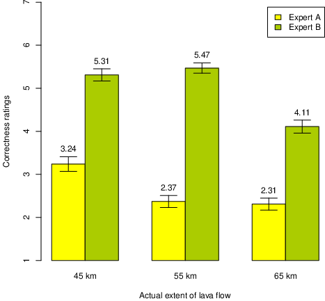
Post hoc accuracy. On a new page, participants read: “Three months later, an eruption took place. It turns out that the lava flow actually extended [45 km] [55 km] [65 km]. How correct were the geologists?” The three distances were chosen to be outside of the interval (above the max value) predicted by Geologist A, and, in three different conditions, lower than the max value, at the max value, and above the max value predicted by Geologist B. The participants rated the predictions of both geologists on a scale ranging from 1 (completely wrong) to 7 (completely correct).

---

Figure 1: Mean correctness ratings (1–7) of predictions from experts with narrow (A: 25–35 km) vs. wide (B: 15–55 km) uncertainty intervals, Experiment 1. (Error bars represent ±1 SEM.)

---

2.2  Results

A large majority found Geologist A, giving a narrow interval, more certain (88.0%) and making use of more advanced prediction models (87.2%) than Geologist B. Providing an interval midpoint did not affect these judgments. Participants with midpoints judged A as more certain (87.3%) and more advanced (84.9%) than B; corresponding percentages were 88.7% and 89.5% for A in the conditions without midpoints. Thus, a general preference for narrow intervals was confirmed, and specifying midpoints did not make a difference.

Post hoc accuracy ratings for the geologists’ predictions are displayed in Figure 1. As there were no significant effects of midpoint, data from the midpoint and no midpoint conditions were pooled. It appears that perceived correctness depended on whether the actual value exceeded the predicted maximum or not. Geologist A with the narrow uncertainty interval, who had in all conditions underestimated the extent of lava flow, was clearly judged more wrong than Geologist B.

Moreover, the correctness of Geologist A’s predictions depended on outcome, as expected, F(2, 247) = 11.42, p < .001. Bonferroni post hoc analyses indicated that A’s predictions of lava flow were more wrong in the 55 km and 65 km conditions than in the 45 km, whereas the 55 km and 65 km conditions did not differ from each other.

The judgments of Geologist B’s predictions were also affected by outcome. A Welch ANOVA¹ yielded a significant effect of outcome on judged correctness, F(2, 153.16) = 25.79, p < .001. This geologist’s predictions were deemed to be more correct for predictions inside than outside of his uncertainty interval. Bonferroni post hoc tests revealed that both inside predictions were significantly more correct than the prediction of a lava flow of 65 km (ps < .001), but not significantly different from each other.

2.3  Discussion

Both experts in the volcano vignette predicted a lava flow of 30 km as the most likely (middle) value, whereas the actual extent turned out to be much higher. This favored the geologist with a wide uncertainty interval, whose predictions were judged to be quite correct, as long as they did not exceed his maximum estimate. Interestingly, they were equally (or more) correct for a flow at the maximum value as for one closer to the center of the interval. Correctness ratings appeared to be based mainly on the relationship between outcome and maximum predictions. Predictions were correct when the outcome fell within the interval, regardless of the interval size, and wrong when they exceeded the upper limit. Interestingly, outcome magnitude seemed only to affect correctness judgments for outcomes outside of the confidence interval.

The vignette in Experiment 1 did not explain why one expert had produced a smaller uncertainty interval than the other. Participants seemed to believe that the expert with narrow interval was more certain and had more advanced prediction models to his disposal. It could, however, be the case that this expert simply did not try to capture all possible values and had produced for instance a 50% interval rather than a 90% interval. In this case there did not have to be a conflict between the two experts. Would outcomes falling outside the 50% interval (but inside a 90% interval) still be regarded as more correctly predicted by an expert with wide intervals? This issue was explored in Experiment 2.

3  Experiment 2

Wide prediction intervals allow a forecaster to be more certain about having captured all possible outcomes in a given prediction task. But people often think otherwise. Løhre and Teigen (2017) found that a large proportion of respondents believed that wide intervals were associated with low certainty, and vice versa, that low-probability prediction intervals would be wider than high-probability intervals. In these studies, participants received specific intervals and filled in an appropriate probability value, or they received specific probabilities and indicated a corresponding prediction interval.

Participants in Experiment 2 received wide and narrow interval forecasts, as in Experiment 1, but the forecasts were this time accompanied by numerical probabilities (confidence levels) showing that the narrow interval was held with low confidence (p = 50%) whereas the wide interval was associated with high confidence (p = 90%). This was expected to make the narrow interval forecasts less certain, and perhaps also less reliable than in Experiment 1, as certainty can now be inferred from the probability estimates rather than from interval ranges. Note that this makes the two forecasts compatible, since a narrow 50% interval can be converted into a 90% interval by moving the interval boundaries outwards. However, if correctness is determined by interval bounds, we expect that expert A with a narrow interval will be perceived as more mistaken (albeit less certain) than expert B with a wide interval, if the actual outcome falls outside of A’s, but inside of B’s interval boundaries. We further expect that all outcomes inside the uncertainty interval would be judged as correct, but that outcomes outside the uncertainty interval might differ in correctness depending upon their distance to the interval boundaries. To include both tails of the distribution, this study included outcomes falling below the lower interval bound in addition to those that exceeded the upper bound.

3.1  Method

Participants were US residents recruited from Mturk. After excluding six respondents who failed an attention check or spent less than 90 seconds on the full survey, 248 participants (120 female, 128 male) remained for analysis. The mean age was 25.3 years (SD = 9.8) and the majority (81.6%) of the participants reported having at least some college education. Participants were assigned to one of four conditions and received the flood predictions question after an unrelated judgment task.

All participants read the following vignette about a flood prediction, borrowed from Jenkins, Harris and Lark (2018).

The Wayston flood plain has a history of flooding due to its flat terrain and proximity to the east side of the river Wayston. A flood within the next few months has been predicted. Two geologists, A and B have been called upon to predict the distance extended by floodwater for this flood, given the river’s situation and recent scientific observations.

Geologist A predicts with 50% probability that the floodwater will extend a distance of 4–7 km from the present east side of the river Wayston.

Geologist B predicts with 90% probability that the floodwater will extend a distance of 2–9 km from the present east side of the river Wayston.

• Which geologist conveys more certainty in his prediction?
• Which geologist do you think makes use of the most advanced prediction models?

Three months later a flood took place. It turned out that the floodwater actually extended [Condition 1: 8 km] [Condition 2: 9 km] [Condition 3: 3 km] [Condition 4: 2 km].

Participants then rated the predictions of both geologists on a scale ranging from 1: completely wrong, to 7: completely correct, as in Experiment 1.

---

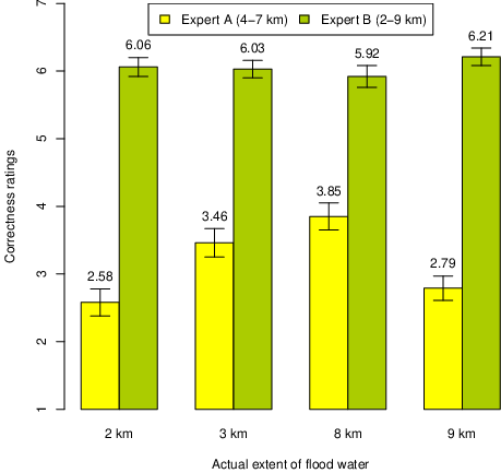
Figure 2: Mean correctness ratings (1–7) of predictions from experts with narrow vs. wide uncertainty intervals, Experiment 2. (Error bars represent ±1 SEM.)

---

Thus, in the High conditions (1 and 2), the extent of floodwater was higher than the midpoints of expected distributions, and in the two Low conditions (3 and 4) it was lower. Moreover, the deviation from expected level was either small or large, forming a 2 x 2 design with direction and magnitude of deviation as the two factors. The distances were chosen to be outside of the interval (above the maximum or below the minimum value) predicted by Geologist A, and inside the interval or at the interval bounds predicted by Geologist B.

3.2  Results

A large majority of participants (86.6%) found Geologist B with the wide interval to be more certain, as this expert reported a much higher confidence in his interval than did Geologist A. They were less in agreement about who used the most advanced prediction model, but a majority (58.3%) favored B in this respect, as well.

The wide predictions of Geologist B were judged to be quite correct in all conditions (overall M = 6.06), regardless of direction and magnitude of deviation, as shown in Figure 2. In contrast, the narrow forecasts of Geologist A were generally considered wrong (overall M = 3.17). A 2 x 2 ANOVA of Geologist A’s ratings revealed no effect of direction (low, high), F(1, 244) = 2.18, p = .14, but a significant effect of magnitude of deviation F(1, 244) = 22.54, p < .001, indicating that small misses are judged less harshly than large misses for outcomes outside of the uncertainty interval.

3.3  Discussion

The results replicated findings from Experiment 1, showing that outcomes inside a wide uncertainty interval are judged to be correct regardless of how much they deviate from the central and presumably most likely value, whereas outcomes above or below the interval bounds are viewed as incorrect, even in the case of a 50% uncertainty interval that does not claim to capture more than the middle two quartiles of the distribution. In the present experiment, the narrow interval was accordingly compatible with the wide interval, which was intended to capture 90% of the outcome distribution. This information was not simply neglected, as it determined the participants’ views about who was more certain, which changed from the narrow forecaster in Experiment 1 to the wide but high probability forecaster in the present vignette. Explicit information about probability (confidence level) might have helped participants to understand the arbitrary nature of upper and lower bounds, which can be placed far apart or closely together depending upon the chosen level. Yet their ratings of correctness seemed to depend exclusively on outcomes falling inside or outside arbitrarily selected interval bounds, demonstrating a strong boundary effect.

4  Experiment 3

The wide and narrow uncertainty intervals used in the preceding studies were centered around the same midpoint, which was assumed to be both forecasters’ most likely estimate. (In Experiment 1 this was stated explicitly in two conditions.) The results indicated that interval bounds were crucial for perceived correctness of the forecasts, implying that distance to most likely estimate is less important. However, a test of this assumption requires a comparison of forecasts with different midpoints. Experiment 3 was undertaken to compare a wide range forecast that captures the target outcome, with a narrower forecast that misses the outcome value, but is better centered. In addition, wide and narrow forecasts were given to different participants in a between-subjects design (as opposed to the two previous studies which allowed participants to directly compare wide and narrow forecasts in a within-subjects design). We also included in this study a test of numeracy and a cognitive reflection test to test the possibility of superficial responses from participants who did not heed or did not understand the probabilistic information.

4.1  Method

Participants were 170 first-year psychology students at two different Norwegian universities, 74.1% female, mean age 22.9 years (SD = 8.1), who participated on a voluntary basis or in exchange for course credits. They performed the correctness judgments as the first of two judgmental tasks in an online questionnaire (powered by Qualtrics). The third part of the questionnaire contained a test of numeracy (Cokely, Galesic, Schulz, Ghazal & Garcia-Retomero, 2012; Schwartz, Woloshin, Black & Welch, 1997) and the Cognitive Reflection Test (Frederick, 2005). This part was completed by only 130 participants.

Participants were randomly assigned to four conditions, according to a 2 x 2 design, with width of interval (wide vs. narrow) and confidence level (specified vs. unspecified) as the two between-subjects factors. The true outcome value was captured by the wide intervals, but not by the narrow intervals. In addition, all intervals contained an expected (most likely) point prediction, which came closer to the true outcome in the narrow than in the wide interval. All participants received both the Flooding and the Volcano scenario, presented in randomized order.

---

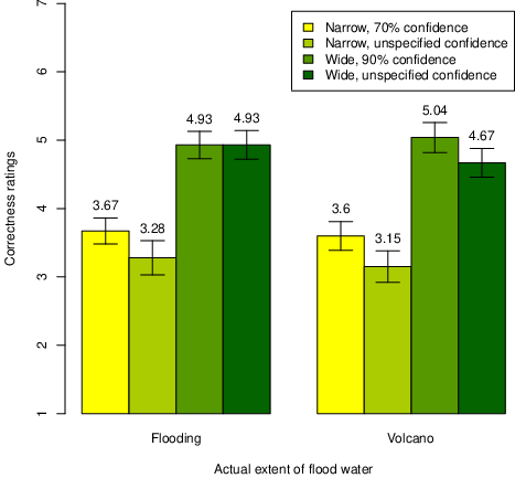
Figure 3: Mean correctness ratings (1-7) of predictions from experts with narrow vs. wide uncertainty intervals for two scenarios, Experiment 3. (Error bars represent ±1 SEM.)

---

1. Flooding Scenario, as in Experiment 2
   1. Wide interval condition: A geologist predicts flood water from the river Wayston extending minimum 2 km and maximum 8 km, with 5 km as the most likely value.
   2. Narrow interval condition: A geologist predicts flood water extending minimum 5 km and maximum 7 km, with 6 km as the most likely value.
   For half of the participants, levels of confidence were not specified. For the other half the wide interval was described as 90% likely and the narrow interval as 70% likely. All participants were told that two months later, a flood took place. It turned out that the flood water actually extended 8 km. How correct was the geologist? (1-7)
2. Volcano Scenario, as in Experiment 1.
   1. Wide interval condition: A geologist predicts a volcanic eruption with the lava flow extending minimum 10 km and maximum 50 km, with 25 km as the most likely value.
   1. Narrow interval condition: A geologist predicts a volcanic eruption with the lava flow extending minimum 20 km and maximum 40 km, with 35 km as the most likely value.
   Again, for half the participants, levels of confidence were not specified, as above. For the other half the wide interval was described as 90% likely and the narrow interval as 70% likely. All participants were told that three months later, a volcanic eruption took place. It turned out that the lava flow actually extended 45 km. How correct was the geologist? (1–7)

4.2  Results

Replicating the results from the previous experiments, participants consistently found the wide interval predictions to be more correct than the narrow interval predictions. Mean accuracy ratings for both scenarios are displayed in Figure 3. The wide interval estimates, whose upper bounds were equal to (Volcano) or slightly higher than (Flooding) the actual outcome, were considered to be more right than wrong, with scores above the scale midpoint, whereas narrow intervals were considered rather inaccurate, even though the most likely values in the narrow ranges were closer to the actual outcome values. Specifying the confidence levels did not appear to make a difference. A 2 x 2 x 2 ANOVA with interval width (wide vs. narrow) and confidence levels (specified vs. unspecified) as between-subjects factors, and scenario (flooding vs. volcano) as a within-subjects factor showed only a significant effect of interval width, F(1,166) = 49.186, p < .001, η_p² = .229, all other F’s < 2.1.

Numeracy and CRT scores from the third part of the questionnaire were available for 130 of the 170 participants (40 participants did not complete this part due to time constraints).² These two measures were positively correlated, r = .454. Numeracy did not appear to reduce the boundary effect.³ Significant positive correlations between accuracy ratings and numeracy were obtained in the condition for wide intervals without confidence level (r = .53 and r = .47 for flooding and volcano, respectively). Similar correlations were obtained between accuracy and CRT in this condition (r = .55 and r = .48), suggesting that numerate participants and participants with a more analytical approach were especially willing to accept interval predictions that captured true outcome values as correct (irrespective of their distance from the most likely estimate).

5  Experiment 4

The actual outcomes given to participants in the three first experiments were rather close to the endpoints of the range (below, above, or equal to the endpoint). However, we cannot claim that all outcomes within a range will be regarded as equally successful “hits”, as we have not sampled outcomes covering the full range, including outcomes closer to the midpoint of the range. Experiment 4 investigated the perceived accuracy of range estimates for central and peripheral outcomes, compared to the perceived accuracy of “most likely” point estimates. We expected range estimates to be less sensitive than point estimates to variations in actual outcomes inside the intervals. We also included ratings of perceived expertise, as the correctness of a single forecast may not be predictive of how likely one is to consult with an expert in the future.

5.1  Method

Participants were 180 first-year psychology students at a university in Southern Norway, 72.8% female, median age 22 years, who participated in exchange for course credits. They performed the correctness judgments as the second of three judgmental tasks in an online questionnaire (Qualtrics). They also answered a test of numeracy, as in Experiment 3. The participants were randomly assigned to four different conditions by receiving different variants of the questionnaires.

All questionnaires contained a vignette presenting forecasts of an expected flood caused by heavy rain and melting of snow in Northern Norway. Heidi Knutsen, hydrologist at NVE (The Norwegian Water Resources and Energy Directorate) said to a local newspaper that the water level in a specific lake, Altevatn, “will most likely increase by 40 cm” during the weekend to come. Tom Djupvik, another hydrologist from the same institute, said to another newspaper that the water level in Altevatn “will most likely increase by 20–60 cm”.

---

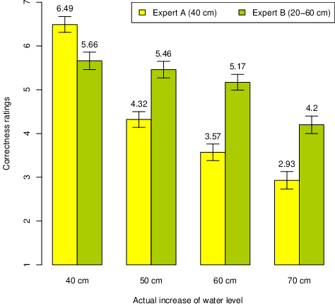
Figure 4: Correctness ratings (1-7) of experts predicting a 40 cm increase or 20–60 cm increase in water level, Experiment 4. (Error bars represent ±1 SEM.)

---

1. Which hydrologist appears more certain in their prognoses? (Heidi Knutsen / Tom Djupvik / Both appear equally certain.)

Participants in four different outcome conditions were then informed that the actual rise in water level was later measured to be [40 cm] [50 cm] [60 cm] [70 cm].

2. How accurate were the forecasts of the two hydrologists? (Rated on a scale from 1: Completely wrong to 7: Completely right.)

3. How do you rate the two hydrologists in terms of apparent expertise (1–7)?

4. How much would you trust the two hydrologists in their future forecasts about flood (1–7)?

Ratings on Scale 3 and 4 were highly correlated (r = .80 and r = .72 for Heidi Knutsen and Tom Djupvik, respectively), so the ratings were averaged to form a Quality of Expert score.

5.2  Results

---

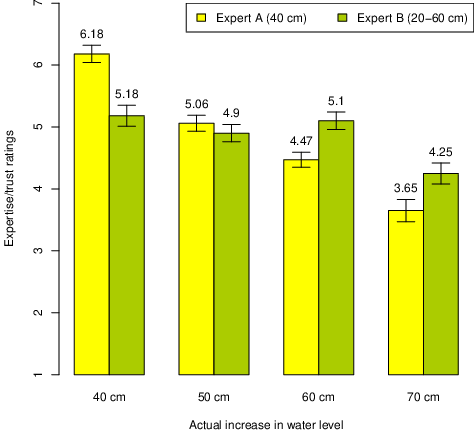
Figure 5: Mean expertise/trust ratings (1–7) of two experts predicting 40 cm or 20–60 cm increase in water level, Experiment 4. (Error bars represent ±1 SEM.)

---

Overall, Heidi Knutsen (henceforth Expert A), who gave a most likely point estimate, was considered more certain by 107 (59.4%) participants, against 36 (20.0%) selecting Tom Djupvik (henceforth Expert B), who gave a most likely range, and 37 (20.6%), who said they were equally certain (after all, they both used the same expression, “most likely” to qualify their estimates). This is in line with the results of Experiment 1, where a wide range indicated higher uncertainty.

Correctness ratings for the two experts are displayed in Figure 4. Expert A is, as predicted, more correct than Expert B when she is spot on, whereas B is seen as more correct at all other outcome values. An overall ANOVA with expert and outcome as the two factors, revealed a main effect of expert, F(1, 176) = 42.14, p < .001, η_p² = .193, and of outcome, F(3, 176) = 53.67, p < .001, η_p² = .478, and more importantly, an interaction, F(3, 176) = 20.91, p < .001, η_p² = .263, confirming that the accuracy profiles of A and B were different from each other. Expert B was considered quite correct in all conditions where his range estimate captured the outcome value. In fact, the ratings in the three first conditions were very similar. Post hoc Bonferroni tests revealed that none of these were significantly different from each other, whereas all were different from mean score in the last condition (all ps < .001). For Expert A, Bonferroni post hoc tests showed significant differences between all adjacent outcome conditions. Her point forecasts were, as expected, poorer the more they differed from the actual outcomes.

This pattern is confirmed by the results of expertise/trust ratings, as displayed in Figure 5. An overall ANOVA with expert and outcome as the two factors showed a strong effect of outcome, F(3, 175) = 33.79, p < .001, η_p² = .367, none of expert, F(1, 175) = 0.44, but again an interaction, F(3, 175) = 18.76, p < .001, η_p² = .243. In this case B’s expertise appears to be the same regardless of outcome, as long as it falls inside his range (Bonferroni post hoc tests show no significant differences between the first three conditions, whereas the 70 cm condition is different from all of them, all ps < .001).

6  Experiment 5

In the previous experiments, the prediction intervals were probabilistically defined, numerically (50%, 70%, or 90%) or verbally (“most likely”), indicating that outcomes outside of the intervals could not be ruled out. Nevertheless, the forecasts were considered accurate mainly for outcomes falling at or inside the interval bounds and less accurate otherwise. Accuracy judgments inside the range were little (or not at all) affected by magnitude of outcome. It did not seem to matter whether the upper and lower limit were labelled maximum and minimum (as in Experiment 1 and 3), or not given any label (as in Experiment 2 and 4). Experiment 3 showed, in addition, that the position of the most likely value in the prediction interval, was considered relatively unimportant. In contrast, the most likely value became important when announced without a prediction interval, as shown in Experiment 4.

It is not obvious whether the forecasts in these experiments should be viewed as being in agreement or disagreement with each other. For instance, the two hydrologists in Experiment 4 came from the same research institute, and the interval forecast of Expert B was centred around the value stated to be “most likely” by Expert A, indicating compatibility. However, we do not know whether Expert A on her part would endorse the range announced by Expert B. In Experiment 5 we introduced a common range but let the two experts differ in the way they chose to phrase their forecast. While one of them suggested the “most likely” outcome, the other chose an outcome that “can” (could) happen.

We expected the “most likely” forecast would be a forecast in the middle of the range, so if the experts agree upon a 20–60 cm water level increase in Altevatn, most participants would think that Expert A has 40 cm as her “most likely” outcome. In line with the results from Experiment 4, we expected accuracy ratings of this forecast to reflect the distance between this value and the actual outcome.

Outcomes that “can” (could) happen are, in principle, all outcomes with a non-zero probability of occurrence, in other words all outcomes within the predicted range. However, in practice, it appears that people use this verb in a more specific sense, selecting an extreme value, typically the top outcome in a distribution of outcomes (Teigen & Filkuková, 2013). We accordingly expected that Expert B would chose 60 cm as a water level rise that “can” occur.

Yet can is an elastic term that does not have the same sharp boundary connotations as the maximum. People who were asked to specify a global temperature increase that can occur, chose the highest value from a family of future projections. Another group in the same study selected the same value as their “maximum” (Teigen, Filkuková & Hohle, 2018). Yet the probability judgments of these two overlapping values were not the same. What can happen was perceived as more likely than a numerically equal outcome termed the maximum. Can (and its cognates, like could and may) is an uncertainty term with positive directionality, in the sense that it directs the listener’s attention towards the occurrence of the target event rather than its non-occurrence (Honda & Yamagishi, 2017; Teigen & Brun, 1995). We accordingly expected that forecasts with can would not be regarded as completely wrong even when the actual outcome value exceeds the forecasted value.

The present experiment investigated these conjectures by presenting people with a prediction interval, asking them what they thought an expert would say would be the most likely (expected) level to occur and what they thought another expert would suggest as a level that could occur. We expected them to answer the first question with a middle value and the second with a high one. Second, they were informed about outcomes inside and outside of the implied range and rated the accuracy of the forecasts. We expected can-statements to be regarded as correct even for outcomes that exceeded the range.

6.1  Method

Questionnaires with valid answers were obtained from 195 students (57 male, 128 female,10 unreported; median age 20 years) attending a lecture in introductory psychology at a university in northern Norway (12 questionnaires were discarded by not conforming to instructions about responding with a single number or entering “wild” responses). The participants were randomly assigned to four different conditions by receiving different variants of the questionnaires.

All questionnaires contained a vignette similar to the one used in Experiment 4. Experts from NVE (The Norwegian Water Resources and Energy Directorate) have estimated that the water level in lake Altevatn will increase by 20–60 cm during the weekend to come, due to heavy rain and melting of snow in northern Norway. On this basis, two hydrologists at NVE make the following predictions (fill in a number that seems appropriate):

Heidi Knutsen (A): “The water level in Altevatn will most likely increase by …cm”

Tom Djupvik (B): “The water level in Altevatn can rise by …cm”.

Participants in four different conditions were subsequently told that the actual rise in water level was later measured to be [40 cm] [50 cm] [60 cm] [70 cm]. They then rated the accuracy of the two hydrologists’ forecasts on two seven-point scales, from 1: Completely wrong, to 7: Completely right.

---

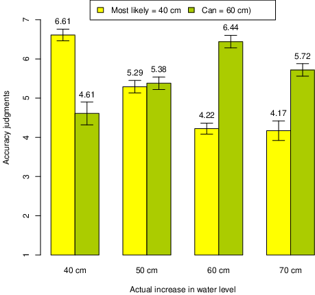
Figure 6: Accuracy judgments (1–7) of expert statements about “most likely” (40 cm) rise in water level and a rise that “can” (60 cm) occur, conditioned upon magnitude of actual outcome. (Error bars represent ±1 SEM.)

---

6.2  Results

Modal estimate of A’s “most likely” forecast was 40 cm (50.3% of all answers), as expected. Mean estimate was lower (M = 34.5 cm), as participants considered increases of 20 and 30 cm to be more likely than values in the upper part of the predicted range.

Modal estimate of B’s forecast of what “can” happen was 60 cm (79.0% of all answers), mean estimate = 55.6 cm. Numbers in the lower part of the distribution were rarely mentioned (< 10%). This is in line with the extremity effect of can (Teigen & Filkuková, 2013; Teigen, Filkuková & Hohle, 2018), which predicts that can is typically used to designate the topmost value in a distribution.

Both forecasts are compatible with the agency’s range estimate of 20–60 cm, and it is reasonable to believe that the respondents assumed that the two experts, coming from this agency, also agreed with each other. They might accordingly be viewed as equally accurate. However, they were rated equal only in the 50 cm condition. With a lower outcome (40 cm) Expert A was seen be more accurate, and for higher outcomes (60 and 70 cm), B’s estimates were judged as more correct. Figure 6 shows mean accuracy judgments for participants who estimated A’s most likely-forecast to be 40 cm and B’s can-forecast to be 60 cm. The figure also shows that A’s forecast became progressively less correct with increasing outcomes, whereas B’s forecast was considered correct not just for outcomes inside the prediction interval, but even for an outcome (70 cm) that exceeded the upper bound.⁴

6.3  Discussion

A forecast of a 20–60 cm rise in water level can be described as an increase of most likely 40 cm, or as an increase of 60 cm that can occur, but the perceived accuracy of these statements is not the same. The first statement will be regarded as correct with medium outcomes (close to 40 cm) and the second as more correct with higher outcomes (closer to 60 cm). The correctness of these statements seems to be judged simply by the distance between the numeric estimate and the actual outcome, even in a context where these estimates had been suggested by the participants themselves as different ways of characterizing the same range of outcomes. The previous studies showed that people regard outcomes beyond the “maximum” level to be inaccurately predicted. In the present study, they use can to describe the maximum level, but evidently in a less categorical way, as in this case a 70 cm outcome, falling outside of the range, is judged to be reasonably well predicted. Thus, can is used to describe a top value without ruling out outcomes that are even more extreme.

7  General discussion

A large amount of research on “credible intervals” and confidence in interval estimates has measured the accuracy of such estimates by comparing assigned or reported confidence levels to the percentage of actual outcomes falling inside the interval bounds. As a result, forecasters who claim to be 80% sure about their intervals, but capture only 36% of actual values, are held to be miscalibrated (Ben-David, Graham, Campbell & Harvey, 2013), and more specifically: overconfident (Soll & Klayman, 2004), or over-precise (Moore & Healy, 2008). This model for assessing calibration rests on the presupposition that all outcomes falling inside the prediction interval can be considered hits, whereas all outcomes outside the interval borders belong to the category of misses, in other words: a binary (dichotomous) concept of what is a correct and what is an incorrect judgment. The present research questions the general acceptability of this classification by asking participants a graded rather than a binary question, namely how correct or how wrong is a prediction, as judgments on a rating scale. For point predictions, we find (as we might expect) that people think of accuracy as a graded concept, depending on the forecast’s closeness or distance from the actual outcome, as indicated by the evaluations of Expert A’s predictions in Figure 4 and 6. For interval predictions, the situation is more complicated, as evaluators have a choice between several reference values, including the most likely estimate and the upper and lower interval bounds. Experiments 1–4 show that the introduction of interval bounds contributes strongly to transforming the question of graded accuracy into a binary question about hits and misses. Outcomes inside a prediction interval are considered hits, even when peripheral or equal to the boundary values, whereas outcomes outside of these boundaries (even when close to them) are considered misses. Figure 1 and 2 indicate, however, that such misses can be graded depending on their closeness to the bounds, whereas outcomes inside the interval are counted as more equally correct.

Such judgments should not come as a surprise, as they may simply indicate that lay people think of hits and misses in a categorical fashion in much the same way as researchers do. (Alternatively, this could be reframed as criticism of research practice in the field, by our pointing out that researchers think much in the same categorical fashion as lay people.) Participants in the present studies tended to stick to the categorical approach even when it was made clear that the upper and lower bounds are not absolute, but rather corresponding to arbitrary points of a distribution (corresponding to 50%, 70%, or 90% intervals).

It is debatable whether, or when, one should regard such effects of categorization as normative or not. It could be claimed that technically, all outcomes that fall inside of the predicted range (regardless of how central they are) should be regarded as “hits” and accordingly as being correct to the same degree, whereas outcomes outside of this range are clearly incorrect, as they were not predicted to occur. On the other hand, it seems equally (or perhaps more) sensible to assess accuracy as a function of the distance between most likely and obtained outcome, even in the case of ranges.

Yaniv and Foster (1995) have argued that, when people receive wide and narrow interval estimates, they are sometimes more concerned about informativeness than accuracy. Hence, when informed that the actual air distance between Chicago and New York is 713 miles, 90% of their participants preferred the incorrect, but informative estimate of 730-780 miles over the technically correct, but uninformative estimate of 700-1500 miles. This suggests that under some circumstances people will prefer narrow range estimates to wide range estimates, even in retrospect. A similar finding was reported by McKenzie and Amin (2002), who showed that people can be sensitive to the “boldness” of a prediction. Participants were told that two students made different predictions about the height of the next person who would come in to the room, with one student predicting a person over 6 feet 8 inches and another predicting a person under 6 feet 8 inches. When informed that the next person was in fact 6 feet 7 inches tall, most people preferred the bold (over 6 feet 8 inches), but incorrect prediction. In both these cases, the technically incorrect, but narrow (or bold) ranges barely missed the correct value, whereas the wide interval barely included it. Observe that participants in these studies were asked about preference, not accuracy, and that the non-preferred intervals were not just wide, but quite misleading. The results suggested, in Yaniv and Foster’s terminology, a “trade-off between informativeness and accuracy”, rather than a general dominance of either of these factors. Their findings are accordingly compatible with our results. In a similar vein, we found in Experiment 5 that out-of-range outcomes were considered fairly accurately predicted by statements about outcomes that “can” occur, as such statements draw attention to (are informative about) high values even when falling short of predicting an actual, out-of-range outcome.

The results fit well with other findings from the research literature on categorization within other domains, including accentuation theory in social cognition (Eiser & Stroebe, 1972). This theory proposes that when a continuous variable is split into categories, the perception of stimuli within these categories change. The differences between items below and items above a category boundary are typically accentuated, whereas members of the same category are judged to be more similar to each other (Tajfel & Wilkes, 1963). The phenomena of within-group homogeneity (assimilation) and between-group accentuation (contrast) have been demonstrated in several areas, both with natural and arbitrary category boundaries, for a variety of tasks, spanning from estimated temperatures in different months of the year (Krueger & Clement, 1994) to estimated similarities between politicians coming from different fractions of the left-right scale (Rothbart, Davis-Stitt & Hill, 1997).

The present studies show assimilation and contrast effects of categories within a new domain, namely in accuracy judgments of range forecasts of environmental risks. Such judgments differ from those studied in the social cognition literature by being more explicit about the homogeneity/heterogeneity of members within a predicted category. Thus, a range prediction about a flood extending 2–8 km indicates that this “category” includes floods of very different magnitudes. Moreover, it is obvious that flood extension is by nature a continuous rather than a discontinuous variable, and that the prediction boundaries are created spontaneously in response to a prediction question, defining an ad hoc category (Barsalou, 1983). An individual forecaster defines the category according to his discretion, and might have placed them differently under different instructions. The boundaries might have been closer together if the forecaster had been asked to be as informative as possible (Yaniv & Foster, 1995), and perhaps wider apart if the forecaster had been required to be 100% certain (although assigned degree of confidence appears to have very little effect on interval width, see Langnickel & Zeisberger, 2016; Teigen & Jørgensen, 2005). Despite the arbitrary placement of interval bounds, the present experiments show that they play a decisive role in perceiving forecasts to be right or wrong. Outcomes within the range are seen to be successfully predicted even when lying at the border, demonstrating an assimilation (homogeneity) effect in the realm of forecast evaluations. Outcomes outside of this interval were judged to be wrong. Interestingly in this case we did not observe a homogeneity effect, as they were judged as more inaccurate the more the outcome deviated from the limits of the uncertainty interval.

The effects of categorization can be further strengthened by introducing category labels (Foroni & Rothbart, 2012; Pohl, 2017), which may also serve to make numerical outcomes more “evaluable” (Hsee & Zhang, 2010; Zhang, 2015). Such labels provide linguistic cues that may serve to increase homogeneity within the category and accentuate the difference between category and non-category members (Hunt & Agnoli, 1991; Walton & Banaji, 2004). For range predictions categorization effects might be accentuated by describing the interval forecast in terms of “expected” (or likely) versus “unexpected” (or unlikely) outcomes. Conventional ways of expressing ranges may by themselves provide a strong categorization cue by highlighting the endpoints. A forecasted flood extending “4–7 km” may appear as forming a more definite interval than a list of “4, 5, 6, or 7 km” as likely or potential values. In Experiment 1 and 3 the boundary values were explicitly labeled minimum and maximum values. With other, more fuzzy and relative terms (like “high” vs. “low” or “optimistic” vs. “pessimistic” estimates) one might expect less of a contrast between accuracy judgments for outcomes falling outside or between the stated values. The present findings are especially relevant for estimation practices in domains that explicitly define maximum and minimum boundaries probabilistically (e.g., in terms of 95% or 80% confidence intervals), as is widely done in project management (Jørgensen, Teigen & Moløkken, 2004; Moder, Phillips & Davis, 1995).

The present studies were exclusively concerned with predictions of a single outcome. Uncertainty intervals for forecasts addressing multiple or repeated outcomes may be easier to understand, especially if presented in a graphical format. Joslyn, Nemec and Savelli (2012) gave participants interval forecasts graphics about temperatures and found that non-experts were able to draw reasonable inferences about variations in future weather. They also found that 80% predictive intervals increased trust in forecaster.

In more informal contexts, forecasts are often made as single-limit intervals, which only specifies the upper or the lower bound, but not both. A geologist may say that the flood will most likely extend “at least 4 km”, without mentioning the upper limit, and an open access journal may assure its authors that it takes (normally) “less than two months” to have their papers published. Again, we may expect that outcomes below the lower limit or above the upper limit will make an observer feel that the predictions were wrong, but not much is known about how forecasts are evaluated when outcomes are close to, or further away from the predicted bound. Will for instance a flood extending 5 km be judged as more, or less correct than a much larger flood, extending 8 km or more? Upper and lower bounds can further be described by inclusive terms (e.g., “minimum”, “at most”), where the interval bounds explicitly form parts of the interval, or by exclusive terms (e.g., “more than”, “below”), which strictly defined do not belong to it. Such choices of term may affect subsequent judgments of accuracy (Teigen, Halberg & Fostervold, 2007). As single-bound estimates are a common, but understudied way of expressing uncertain forecasts, we think that such a line of research would be worth pursuing.

7.1  Conclusion

Range predictions carry several messages, not all of them intended by the forecasters. In contrast to point predictions, ranges communicate a degree of uncertainty, or vagueness. But ranges have boundaries, which taken literally may be read as demarcation points. The present studies give evidence for a weaker and a stronger version of a boundary effect: (a) boundaries create a dividing line between accurate and inaccurate predictions, even for ranges that are probabilistically defined; (b) boundaries can make all predictions within the range appear equally correct. Yet, as our final study showed, people can be sensitive to labels chosen by the forecaster. Top values described as outcomes that “can” occur evoke no boundary effect.

References

*

Department of Psychology, University of Oslo, P.b. 1094 Blindern NO-0317, Oslo, Norway. Email: k.h.teigen@psykologi.uio.no.

#

Simula Research Laboratory, Oslo, Norway

This research was supported by Grant No.235585/E10 from The Research Council of Norway.

Copyright: © 2018. The authors license this article under the terms of the Creative Commons Attribution 3.0 License.

1

Levene’s test was significant, F(2,247) = 3.22, p < .041

2

Analyses of accuracy judgments based on the 130 participants who completed all parts of the questionnaire yield the same pattern of results as those based on the total sample.

3

Participants with high numeracy (according to a median split) distinguished even more sharply between narrow and wide intervals. A 2 x 2 x 2 ANOVA for flooding yielded a significant interaction effect between numeracy (high vs. low) and interval, F(1, 130) = 5.91, p = .016, η_p² = .043; a similar analysis for accuracy ratings for the volcano scenario yielded an even stronger effect, F(1, 130) = 13.36, p < .001, η_p² = .093.

4

An analysis including all estimates (not limited to participants that suggested 40 cm for most likely and 60 cm for can) yielded similar profiles to those displayed in Figure 6. A mixed ANOVA gave a significant main effect of Expert, F(3, 191) = 56.251, p < .001, η_p² = 0.122, indicating that can is generally more accurate than most likely, and more important, a significant interaction between Expert and Condition, F(3,191) = 19.01, p < .001, η_p² = 0.233, confirming the difference in profiles of the two experts.

This document was translated from L^AT_EX by H^EV^EA.