Hierarchical Bayesian modeling of intertemporal choice

There is a growing interest in studying individual differences in choices that involve trading off reward amount and delay to delivery because such choices have been linked to involvement in risky behaviors, such as substance abuse. The most ubiquitous proposal in psychology is to model these choices assuming delayed rewards lose value following a hyperbolic function, which has one free parameter, named discounting rate. Consequently, a fundamental issue is the estimation of this parameter. The traditional approach estimates each individual’s discounting rate separately, which discards individual differences during modeling and ignores the statistical structure of the population. The present work adopted a different approximation to parameter estimation: each individual’s discounting rate is estimated considering the information provided by all subjects, using state-of-the-art Bayesian inference techniques. Our goal was to evaluate whether individual discounting rates come from one or more subpopulations, using Mazur’s (1987) hyperbolic function. Twelve hundred eighty-four subjects answered the Intertemporal Choice Task developed by Kirby, Petry and Bickel (1999). The modeling techniques employed permitted the identification of subjects who produced random, careless responses, and who were discarded from further analysis. Results showed that one-mixture hierarchical distribution that uses the information provided by all subjects suffices to model individual differences in delay discounting, suggesting psychological variability resides along a continuum rather than in discrete clusters. This different approach to parameter estimation has the potential to contribute to the understanding and prediction of decision making in various real-world situations where immediacy is constantly in conflict with magnitude.

Keywords: intertemporal choice, hierarchical modeling, delay discounting, Bayesian inference, parameter estimation.

1 Introduction

Organisms often choose between rewards that differ in magnitude and delay to delivery. How they trade off these features is important in understanding and predicting people’s intertemporal choices, which can be defined as decisions whose outcomes occur at different points in time (Frederick, Loewenstein & O’Donoghue, 2002).

The study of intertemporal choices has real-world implications because many crucial decisions that affect people’s quality of life are intertemporal tradeoff dilemmas that ultimately affect public policy and economic markets (Andreoni & Sprenger, 2012). Research has found that individual differences in time preferences are connected to engagement in risky behaviors, such as substance abuse. Previous reports suggest that abusers of substances such as tobacco (Bickel, Odum & Madden, 1999), alcohol (Petry, 2001), and heroin (Kirby, Petry & Bickel, 1999), tend to prefer rewards sooner than non-drug users, meaning the former place greater importance on immediacy rather than magnitude when solving intertemporal dilemmas.

The time preference literature has developed different models to explain how organisms represent and evaluate the options available in their choice space. The most commonly used proposal in psychology is the one-parameter hyperbolic function (Mazur, 1987), which rests on the following assumptions:

According to Mazur’s (1987) hyperbolic function, rewards are compared in terms of their subjective values, which are determined by the following equation:

where V represents the subjective value of a certain amount A delayed D time units. The free parameter, k, known as discounting rate, represents the rate at which the amount A losses value as time to its delivery increases. Note that for immediately available rewards, the delay D equals zero, and the subjective value V equals monetary amount A.

That rewards are discounted hyperbolically means not only that valuation changes as time progresses but also that the proportion by which it changes varies continuously (Killeen, 2009). This function’s success resides in its ability to account for a ubiquitous dynamic inconsistency: that people’s original preference reverses as the temporal distance to both outcomes decreases (Ainslie, 1975; Cheng & González-Vallejo, 2016).

Because differences in choice behavior are assumed to associate with differences in discounting rate, k, the estimation of this parameter is a central issue (Green, Fry & Myerson, 1994; Killeen, 2009). The traditional way to model heterogeneity in choice is by fitting a discounting function to each subject’s data separately, and estimating a fixed discounting rate per person (Bickel, Odum & Madden, 1999; Green, Myerson & McFadden, 1997; Madden, Raiff, Lagorio, Begotka, Mueller, Hehli & Wegener, 2004). Statistically, this approach rests on the idea that the only information required to estimate any subject’s k is the data each person provides.

A second, richer approach assumes subjects originate from an overarching distribution, meaning they are related to one another. Vincent (2016) presents an example of this perspective. He estimated trial-, subject- and group-level parameters simultaneously, using hierarchical modeling. The success of this technique in cognitive modeling stems from a particular treatment of between-subject variability that neither ignores nor overweights individual differences: the estimation of parameter values for each subject is informed by the information contributed by the rest of the individuals (Nilsson, Rieskamp & Wagenmakers, 2011).

The present work introduces a natural extension to the hierarchical approach adopted by Vincent (2016): the possibility of modeling differences in delay discounting as a combination of N sub-population distributions. In this type of representation, called latent mixture model, the mixture component captures qualitative differences among groups of people, while the hierarchical component accounts for the variability within each group (Lee, 2016). For each subject, parameter values are calculated conditional on the distribution they come from (Gelman, Carlin, Stern & Rubin, 2004; Gershman & Blei, 2012). Modeling individual differences as a mixture of different processes is common in fields such as medical diagnosis, where measurable individual variables are used to allocate people into clusters (Bartholomew, Steele, Moustaki & Galbraith, 2008), and has multiple real-world applications. Examples from the substance abuse literature highlight the potential clinical value of discounting rates to predict whether abstinent smokers will relapse (Dallery & Raiff, 2007; Yoon, Higgins, Heil, Sugarbaker, Thomas & Bader, 2007).

Besides endorsing a specific statistical model, an equally relevant issue in parameter estimation is the choice of inference procedures. The challenge is the handling of the uncertainty linked to estimating parameter values from limited data. Bayesian methods are a viable alternative to traditional inference techniques to address this challenge, as they offer a coherent and consistent response to the inference problem. The literature provides evidence that Bayesian techniques result in more robust parameter estimates, as has been demonstrated in simulation studies where data-generating parameter values were recovered more accurately and with less variability via Bayesian methods than via more traditional approaches, such as maximum likelihood estimation (MLE). In addition to their robustness, Bayesian methods can be more informative than traditional techniques because they supply full posterior distributions over parameter values instead of only point estimates (Nilsson, Rieskamp & Wagenmakers, 2011).

Another key advantage of Bayesian inference comes from the possibility of fitting a wider set of models, as the same and unique principle of inference — Bayes’ Rule — can be applied flexibly to both simple and complex structures. We illustrate this advantage by building a model aimed at identifying subjects who use some cognitive process other than the one of interest to produce behavior in a task. Factors such as lack of attention or motivation can originate careless responses. Because such responses do not represent the behavior of interest, recognizing subjects who produce them represents a major advantage not only for parameter inference but also for the study of individual differences (Lee, 2016; Zeigenfuse & Lee, 2010).

Therefore, the present work offers a description of individual variation in a delay discounting task by implementing two analyses: one that compares different hierarchical, population-level distributions over hyperbolic discounting rates, and another that detects subjects who responded the task carelessly, in order to prevent them from affecting parameter inference.

2 Method

2.1 Subjects

As part of a broader project that studied risky decision making as a case of choice behavior, 1284 Mexican students (629 females) participated in the study as a class requirement. The sample was composed mainly of high school juniors and seniors (87%) and included some first-year university students (13%).

2.2 Materials and Procedure

The Intertemporal Choice Task (Kirby, Petry & Bickel, 1999) consists of 27 trials, each of which presents a choice between two hypothetical monetary rewards, one smaller in amount and available immediately (named SS) and another larger in amount, available after a certain delay (called LL). We employed this instrument because of its extensive use within the temporal discounting literature, which largely stems from the questionnaire’s adequate psychometric properties (Kirby, 2009; Myerson, Baumann & Green, 2014). Monetary amounts were as stated by the authors (but expressed as Mexican pesos instead of U.S. dollars), delays were expressed as number of days to delivery and trials were presented in the order specified by the authors.

3 Bayesian Data Analysis

We analyzed the process underlying choice data by applying four models using the Bayesian framework.

The first model was designed to distinguish subjects who behave according to the hyperbolic model (henceforth, “non-contaminant subjects”) from whose who produced careless, random responses (“contaminant subjects”). The remaining three models consist of hierarchical extensions that assume individual discounting rates come from either a one-mixture, a two-mixture, or a three-mixture population distribution, respectively.

The contaminant-detector model allowed us to identify 109 individuals who responded randomly; these subjects were excluded from further analysis. On the other hand, the comparison among the mixture models suggested hyperbolic discounting rates are better described by a single, one-mixture population distribution.

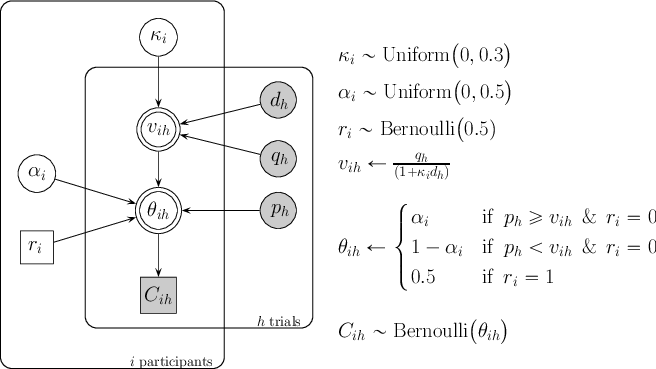
We follow the notation presented in Lee (2008)¹ to detail all models. In this representation, shaded nodes correspond to observed variables, whereas unshaded nodes stand for latent variables. Double-bordered nodes are deterministic, while single-bordered nodes are stochastic. Circles represent continuous variables, and squares portray discrete variables. Each model contains two bounding rectangles that enclose independent replications of two structures within the model: one corresponding to subjects i, and the other representing trials h.

The main analysis code was written in R. We used JAGS (Just Another Gibbs Sampler; Plummer, 2003) to conduct Markov chain Monte Carlo sampling-based inference. For all nodes in all models, posterior distributions were estimated drawing a total of 500,000 samples over 2 chains. The first 200,000 samples were discarded (the burn-in interval), and only one sample of each 300 was retained for a total of 1,000 final samples per chain. Under these sampling parameters and given the size of our dataset, each model took about 30 hours to run. Convergence was verified by visual inspection of the chains and by computing the R statistic (Gelman & Rubin, 1992). Around 95% of nodes within each model showed R values between 1 and 1.05, which is traditionally interpreted as a sign of reliable convergence between chains.

3.1 Detecting Contaminants

The core model, common to the contaminant-detector and to all mixture models, assumes each subject i has a discounting rate k_i.² For each trial h, the subject’s discounting rate determines the subjective value of LL, v_ih, combining its delay d_h and monetary quantity q_h according to Mazur’s hyperbolic equation. Next, the model decides whether v_ih is greater or less than the value of the SS alternative, p_h. If p_h ⩾ v_ih, the model concludes the probability of choosing the LL reward lies between 0 and 0.5 (i.e., it is rather unlikely to choose the LL option if SS has a larger value). On the contrary, if p_h < v_ih, the probability of choosing LL is somewhere between 0.5 and 1.0. Both cases are encoded in node θ_ih, which represents the probability of choosing the LL reward in trial h for subject i.³ The actual response, C_ih, codes SS responses as 0 and LL responses as 1. This model, along with the contaminant-detector extension, is presented in Figure 1.

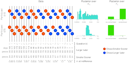
The contaminant-detector extension consists of a third possibility in node θ_ih that intends to identify data generated by psychological processes different from hyperbolic discounting (Zeingenfuse & Lee, 2010). Specifically, the model assumes that θ_ih is low because p_h ⩾ v_ih, large because p_h < v_ih, or that θ_ih=0.5 regardless of the values of the SS and LL alternatives. The first two scenarios correspond to subject i being guided by the amounts and delays of each question in the task, and is represented as r_i=0. The last scenario corresponds to subject i responding randomly, and is represented as node r_i=1. Note that node r_i is unknown and its value is inferred conditional on each subject’s data. Before taking data into account, we assumed each subject was equally likely to be a contaminant or a non-contaminant, which is represented by the uniform prior distribution over nodes r_i.

To illustrate how the contaminant-detector model works, we present two exemplar subjects’ data and the corresponding conclusions of this model in Figure 2. In the left panel, we plotted each subject’s responses coding SS choices as red and LL choices as blue circles. Note that the order of the questions in the figure is guided by the discounting rate value that makes a subject indifferent between both alternatives (k at indifference).⁴

In the top row, subject 815’s responses reveal an unordered and suspicious pattern, visually reflected as blue and red dots intermixed across the whole question set. Take questions 1 and 24 as examples. In question 1, this subject chose the LL reward, which suggests $55 in 117 days has a larger subjective value than $54 immediately. However, the same subject chose the SS reward in question 24, which indicates $60 in 111 days has a smaller subjective value than $54 immediately. Both responses imply $60 in 111 days < $55 in 117 days. According to the hyperbolic model, choosing a smaller monetary amount delivered later over a larger amount of sooner delivery is inconsistent behavior. A similar inconsistency occurred between questions 19 and 4. In the former, $80 in 14 days were preferred over $33 with no delay; in the latter, $31 delivered immediately were chosen over $85 in 7 days. In summary, the responses of subject 815 are inconsistent with a single discounting rate value, and therefore suggest her behavior is not guided by the amounts and delays the task presents.

As a consequence, the contaminant-detector inference over subject 815’s discount rate, presented in the middle panel, reflects high posterior uncertainty. Since the responses from this subject are consistent with several k₈₁₅ values, the uniform prior is barely updated by her choices and the model is inconclusive regarding her discounting rate. Accordingly, the model concludes it is more likely that this subject responded randomly, which is represented in the posterior distribution over node r₈₁₅ (top row, right panel). In other words, based on this subject’s choices, the contaminant-detector model was able to infer subject’s 815 responses were more likely produced by chance rather than being guided by the set of alternatives in the questionnaire.

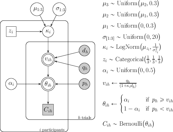
In contrast, subject 675 (bottom row) presents an ordered pattern of responses. With the exception of questions 16 and 18, SS and LL choices appear at the left and right regions of the plot, respectively, which suggests this subject’s discounting rate at indifference lies somewhere between 0.016 and 0.041. Since most responses are consistent with a small set of possible discounting rates, the posterior distribution over k₆₇₅ assigns more density to a reduced region of the parameter, automatically discarding extreme values. The consistency among this subject’s choices and the narrow posterior distribution over her discounting rate are in line with the posterior distribution over node r₆₇₅, which strongly indicates this subject did not respond randomly, and was rather guided by the amounts and delays of each alternative in the task.

In sum, the contaminant-detector model was able to identify noise produced by the stochastic nature of choice, such as questions 16 and 18 for subject 675, and distinguish it from noise produced by responding the task carelessly, exemplified by subject 815’s responses.

We decided which subjects produced contaminant responses by computing their posterior means over the contaminant-detector node. Every subject whose posterior mean over node r_i was larger than 0.5 was labeled “contaminant”. Under this criterion, we identified 109 contaminants (8.5% from the total sample) that were discarded from further analysis.

3.2 Mixture models

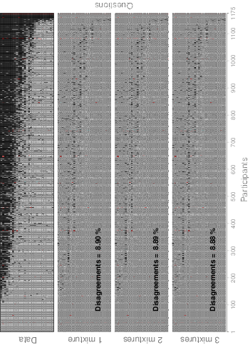
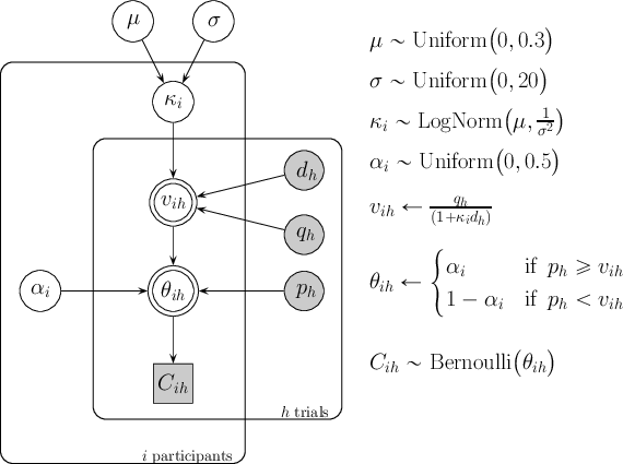
The models portrayed in Figures 3 and 4 consider subjects come from either one, two or three group-level distributions with respect to their discounting rate. The second model, portrayed in Figure 3, expands the basic structure of the core model, assuming k is governed by a group-level distribution⁵ with parameters µ and σ.

The two remaining models, both depicted in Figure 4, extend the hierarchical structure to assume the group-level distribution is composed of two and three mixtures, respectively. These models estimate individual group membership (represented by categorical variable z_i) as well as the parameters that govern each mixture in the overarching hierarchical distribution. In other words, the two-cluster model represents the possibility that there are two different subpopulations of discounters, each characterized by its own parameter values: µ₁ and σ₁, and µ₂ and σ₂. Similarly, the three-cluster model assumes an additional subpopulation of discounting rates, and infers the parameter values that govern each distribution: µ_1:3 and σ_1:3.

Figure 5 contrasts the data (1175 non-contaminant subjects) against the predictions from each mixture model. In each panel, subjects are ordered from left to right with respect to the number of LL choices they made, while questions follow the same order as in Figure 2 (lowest to highest k at indifference) from bottom to top. In Data, white represents an SS choice, while black accounts for an LL choice. Red represents missing data. The leftmost section of the data panel shows a group of 109 subjects (9.28% from the sample) who selected SS in all trials. In contrast, the rightmost section of the panel shows 17 subjects (1.45%) who chose LL in all trials. As for the remaining 89%, two features are worth mentioning: first, the abundant individual differences in the data set; second, that this variability can be described by a relatively smooth line that divides each subject’s SS and LL choices.

The remaining panels in Figure 5 contrast data with the predictions of the three mixture models. While grey areas represent cases in which model prediction and data concur, black and white line segments are cases in which model prediction and data differ. In such cases, the color corresponds to the predicted choice. For example, a white segment indicates the model expected an SS answer, but the subject opted for LL. Furthermore, each panel includes the global percentage of disagreement between data and the model’s prediction. A quick inspection of these percentages makes evident that the two- and three-mixture models do not improve the descriptive adequacy of the one-mixture model substantially, thus suggesting a single overarching distribution suffices to describe the variability in our data.

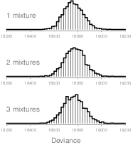
A second reason to prefer the one-mixture model is based on the Deviance Information Criterion (DIC). This is a measure of overall model fit, according to which lower values identify the model with the best out-of-sample predictive power (Gelman et al., 2004). Figure 6 shows the posterior distributions over this model-selection criterion, for each of the mixture models tested. As can be seen, the distribution for the one-mixture model is centered around slightly smaller values. More importantly, the two-and three-group DIC distributions suggest that additional subpopulations do not improve fit.

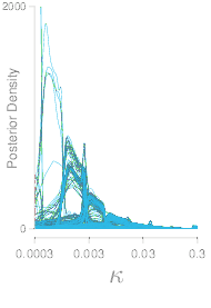
According to the one-mixture model, a full depiction of variation among individual discounting rates is presented in Figure 7. Most discounting rates lie at the middle of the range, which largely reflects the fact that most subjects switch from SS to LL choices around half the questionnaire. A small set of k_i’s with high posterior density at the extremes corresponds to subjects that chose mostly SS (highest k_i’s) or LL (lowest k_i’s) alternatives.

To examine individual differences in greater detail, Figure 8 portrays data, discounting rate and the corresponding discounting function for three subjects. These subjects were selected precisely because they represent the diversity found in our dataset. The structure of Figure 8 is the same as that of Figure 2, with the exception that Figure 8 discards the contaminant-detector node and instead presents the inferred discount function, which exemplifies how the subjective value of a $90 reward decreases when its delivery is delayed. Note that we have plotted several likely curves to account for posterior uncertainty over each individual’s discounting rate.

The subject portrayed in the top row selected the LL alternative in 78% of the trials, but opted for the SS alternative in 22% of the trials in which the delay to the LL alternative implied a substantial waiting period (over 100 days). The posterior distribution of her discounting rate is located at the low extreme of the discounting continuum. For her, a $90 reward would not suffer a drastic loss of value, even after a delay of 300 days.

The person shown in the middle row selected the SS alternative in 52% of the trials, but chose LL in the remaining 48% of the trials. This subject opted for the LL reward in trials with a short delay to delivery (30 days or less). Consistent with the observed choices, this subject’s posterior distribution over k is situated in the middle portion of the region. For this person, a $90 reward would lose most of its subjective value after 150 days.

Finally, the subject portrayed in the bottom row chose the SS reward in most trials (82%). The trials in which she selected the LL reward imply a short delay to delivery (14 days or less). Accordingly, her discounting rate lies at the high extreme of the continuum. In her case, a $90 reward would have almost no subjective value if its delivery is even slightly delayed.

4 Discussion

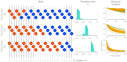
The present work provides evidence that individual differences in a delay discounting task can be successfully modeled assuming subjects originate from one group-level distribution. While time preferences research has acknowledged the importance of providing more precise measurements of individual differences in discounting (Myerson, Baumann & Green, 2014), these differences have traditionally not been incorporated into the modeling of intertemporal choices. That variability in delay discounting can be modeled with one overarching distribution is theoretically relevant and suggests interindividual heterogeneity can be located along a continuum scale, and therefore can be described by the same underlying psychological process.

Although we did not find evidence of different subpopulations of individuals within our sample, it is worth highlighting the dataset was large enough to find them, if they were present. Nevertheless, the modeling approach we employed holds potential for future research that relates delay discounting in populations that differ in their involvement in risky behaviors such as drug abuse, credit card debt, gambling, among others.

It is worth noting the present work did not intend to compare the adequacy of different delay discounting models. We selected Mazur’s hyperbolic function to implement our modeling approach because this equation has been the most commonly used to study the relationship between delay discounting and risky behaviors. However, in recent years, attribute-based models have become an alternative approach to understanding intertemporal choices. These models assume the different features of an alternative are not integrated into a global value, but instead are compared directly (Dai & Busemeyer, 2014; Scholten & Read, 2010; Scholten, Read & Sanborn, 2014). While a detailed discussion on the adequacy of such models escapes the scope of this paper, we suggest intertemporal choice research can largely benefit from using the contaminant-detector extensions and hierarchical-mixture modeling shown in this work.

The Intertemporal Choice Task possesses strengths that have made its use widespread in time preferences research. Firstly, it is quick and easy to administer. Secondly, it has met psychometric standards for reliability and validity. Thirdly, it has proven to capture behavior differences between drug and non-drug users (Kirby, 2009). Despite these advantages, the questionnaire’s scoring method poses complications for parameter estimation. Because individuals are assigned to one of 10 possible k categories, it automatically narrows the measurement of discounting rate, which is implicitly understood as a continuous variable (Myerson, Baumann & Green, 2014). Additionally, because traditional modeling approaches do not consider the possibility that subjects answer randomly, unidentified contaminant data can distort parameter inference. These limitations can be successfully addressed via Bayesian inference methods.

This study and Vincent (2016) are promising examples of the use of Bayesian methods in time preferences research. Bayesian methods prove to be powerful techniques for modeling individual differences in intertemporal decision making. Besides providing more information about parameter estimates than traditional inference procedures, they can effectively identify subjects who produce contaminant responses. By removing the 8.5% of subjects who answered randomly from further modeling, we were able to provide greater precision in parameter estimation at subject- and group-levels, thus allowing for more robust conclusions.

While the present work and Vincent (2016) both use Bayesian methods to estimate parameters in delay discounting, they differ in aspects worth mentioning. As far as general purpose, he aimed to introduce Bayesian estimation and hypothesis testing for delay discounting tasks, while this work seeked to model individual differences assuming subjects come from different subpopulations. In terms of the dataset, he used a small sample of subjects who behaved similarly; by contrast, the present research evaluated a considerably larger number of individuals, providing a dataset especially well suited to research individual differences. Finally, as far as the modeling, he assumed a single group level population, while we explored different group structures to model data.

Studying inter-individual heterogeneity in delay discounting assuming subjects are similar to one another deserves further exploration for two main reasons. Firstly, because this perspective can contribute to the understanding of how people solve intertemporal choice dilemmas. Secondly, because this comprehension has the potential to modify organisms’ consumption choices in several real-world scenarios where the tradeoff between immediacy and magnitude is constantly on the agenda.

References

Ainslie, G. (1975). Specious reward: A behavioral theory of impulsiveness and impulse control. Psychological Bulletin, 82(4), 463–496.

Andreoni, J. & Sprenger, C. (2012). Estimating time preferences from convex budgets. The American Economic Review, 102(7), 3333–3356.

Bartholomew, D. J., Steele, F., Moustaki, I. & Galbraith, J. I. (2008). Analysis of Multivariate Social Science Data. Boca Raton: CRC Press.

Bickel, W. K., Odum, A. L. & Madden, G. J. (1999). Impulsivity and cigarette smoking: delay discounting in current, never, and ex-smokers. Psychopharmacology, 146(4), 447–454.

Cheng, J. & González-Vallejo, C. (2016). Attribute-wise vs. alternative-wise mechanism in intertemporal choice: Testing the proportional difference, trade-off, and hyperbolic models. Decision3(3), 190–215.

Dai, J. & Busemeyer, J. R. (2014). A probabilistic, dynamic, and attribute-wise model of intertemporal choice. Journal of Experimental Psychology: General, 143(4), 1489–1514.

Dallery, J. & Raiff, B. R. (2007). Delay discounting predicts cigarette smoking in a laboratory model of abstinence reinforcement. Psychopharmacology, 190(4), 485–496.

Frederick, S., Loewenstein, G. & O‘Donoghue, T. (2002). Time Discounting and Time Preference: A Critical Review. Journal of Economic Literature, 40, 351–401.

Gelman, A., Carlin, J. B., Stern, H. S. & Rubin, D. B. (2004). Bayesian Data Analysis. Boca Raton: Chapman & Hall/CRC Press.

Gelman, A. & Rubin, D. B. (1992). Inference from iterative simulation using multiple sequences. Statistical Science, 7(4), 457–472.

Gershman, S. J. & Blei, D. M. (2012). A tutorial on Bayesian nonparametric models. Journal of Mathematical Psychology, 56, 1–12.

Green, L., Fry, A. F. & Myerson, J. (1994). Discounting of delayed rewards: A life-span comparison. Psychological Science, 5(1), 33–36.

Green, L., Myerson, J. & McFadden, E. (1997). Rate of temporal discounting decreases with amount of reward. Memory & Cognition, 25, 715–723.

Lee, M. D. (2008). Three case studies in the Bayesian analysis of cognitive models. Psychonomic Bulletin & Review, 15(1), 1–15.

Lee, M. D. (2016). Bayesian methods in cognitive modeling. Submitted for The Stevens’ Handbook of Experimental Psychology and Cognitive Neuroscience. Fourth Edition.

Killeen, P. (2009). An additive-utility model of delay discounting. Psychological Review, 116(3), 602–619.

Kirby, K. N. (2009). One-year temporal stability of delay-discounting rates. Psychonomic Bulletin & Review, 16(3), 457–462.

Kirby, K. N., Petry, N. M. & Bickel, W. K. (1999). Heroin Addicts Have Higher Discount Rates for Delayed Rewards Than Non-Drug Using Controls. Journal of Experimental Psychology: General, 128(1), 78–87.

Madden, G. J., Raiff, B. R., Lagorio, C. H., Begotka, A. M., Mueller, A. M., Hehli, D. J. & Wegener, A. A. (2004). Delay discounting of potentially real and hypothetical rewards: II. Between- and within- subject comparisons. Experimental Clinical Psychopharmacology, 12, 251–261.

Mazur, J. E. (1987). An adjusting procedure for studying delayed reinforcement. In Commons, M. L., Mazur, J. E., Nevin, J. A. and Rachlin, H. (Eds.), Quantitative Analyses of Behavior, 55–73. Erlbaum, Hillsdale, N. J.

Myerson, J., Baumann, A. A. & Green, L. (2014). Discounting of delayed rewards. (A)theoretical interpretation of the Kirby questionnaire. Behavioural Processes, 107, 99–105.

Nilsson, H., Rieskamp, J. & Wagenmakers, E.-J. (2011). Hierarchical Bayesian parameter estimation for cumulative prospect theory. Journal of Mathematical Psychology, 55, 84–93.

Petry, N. M. (2001). Delay discounting of money and alcohol in actively using alcoholics, currently abstinent alcoholics, and controls. Psychopharmacology (Berlin), 154, 243–250.

Plummer, M. (2003). JAGS: A program for analysis of Bayesian graphical models using Gibbs sampling. In: Hornik. K., Leisch, F. & Zeileis, A. (Eds.). Proceedings of the 3rd International Workshop on Distributed Statistical Computing. Vienna, Austria.

Scholten, M. & Read, D. (2010). The psychology of intertemporal tradeoffs. Psychological Review, 117(3), 925–944.

Scholten, M., Read, D. & Sanborn, A. (2014). Weighing Outcomes by Time or Against Time? Evaluation Rules in Intertemporal Choice. Cognitive Science, 38, 399–438.

Vincent, B. J. (2016). Hierarchical Bayesian estimation and hypothesis testing for delay discounting tasks. Behaviour Research Methods, 48(4), 1608–1620.

Yoon, J. H., Higgins. S. T., Heil, S. H., Sugarbaker, R. J., Thomas, C. S. & Bader, G. J. (2007). Delay discounting predicts postpartum relapse to cigarette smoking among pregnant women. Experimental and Clinical Psychopharmacology, 15(2), 176–186.

Zeigenfuse, M. D. & Lee, M. D. (2010). A general latent assignment approach for modeling psychological contaminants. Journal of Mathematical Psychology, 54, 352–362.

Laboratorio 25, Facultad de Psicología, Universidad Nacional Autónoma de México, Av. Universidad 3004 Col. Copilco Universidad Del. Coyoacán, C.P. 04510 Ciudad de México. Email: chavez86unam@gmail.com

A preliminary version of this research was presented as a poster at the 2015 Society for Judgment and Decision Making annual conference. The authors thank Leonard Green, Michael Lee and two anonymous reviewers for their valuable feedback, and gratefully acknowledge the support of CONACyT (104396) and PAPIIT (IN307214).

An introduction to Bayesian philosophy, methods and techniques, along with several worked applications in cognitive science can be found in Lee, M.D. & Wagenmakers, E.-J. (2014). Bayesian Cognitive Modeling: A practical course. Cambridge: Cambridge University Press.

The contaminant-detector model assumes individual discounting rates lie somewhere between 0 and 0.30 because Kirby et al.’s questionnaire is sensitive to k values in that range. See Figure 1 for details on the prior distributions.

In this sense, the node α_i works as an auxiliary node that roughly reflects how strict a subject is when choosing between the two alternatives in each trial.

The actual order of presentation in the paper-pencil instrument is presented as “question id.” (see Kirby et al., 1999, for details).

Since the natural logarithm of the discounting rates is assumed to be normally distributed, we employed log-normal hierarchical distributions over non-transformed k_is in all mixture models. See Kirby et al. (1999) for details.