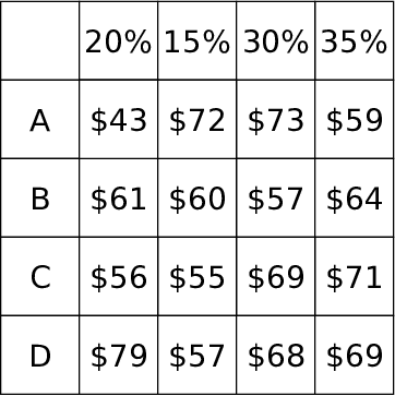
| Figure 1: Example stimulus with all outcome values shown. During a trial, the alternative names (“A”, “B”, etc) and probabilities were always visible. Outcomes selected by the participant were temporarily visible. |
Judgment and Decision Making, Vol. 11, No. 6, November 2016, pp. 611-626
The effect of interruption on the decision-making processCheryl A. Nicholas* Andrew L. Cohen# |
Previous research has shown that interruptions can lead to delays and errors on the interrupted task. Such research, however, seldom considers whether interruptions cause a change in how information is processed. The central question of this research is to determine whether an interruption causes a processing change. We investigate this question in a decision-making paradigm well-suited for examining the decision-making process. Participants are asked to select from a set of risky gambles, each with multiple possible stochastic outcomes. The information gathering process is measured using a mouse-click paradigm. Consistent with past work, interruptions did incur a cost: An interruption increased the time and the amount of information needed to make a decision. Furthermore, after an interruption, participants did seem to partially “restart” the task. Importantly, however, there was no evidence that the information gathering pattern was changed by an interruption. There was also no overall cost to the interruption in terms of choice outcome. These results are consistent with the idea that participants recall a subset of pre-interruption information, which was then incorporated into post-interruption processing.
Keywords: interruption, decision making, process tracing
An interruption is a break that occurs while performing a task with the intention to resume and complete the original task (Boehm-Davis & Remington, 2009; Li, Blandford, Cairns & Young, 2008). Although results are mixed (e.g., Oulasvirta & Saariluoma, 2006), interruptions are typically found to be disruptive and to negatively affect both performance and behavior (Altmann & Trafton, 2004; Altmann, Trafton, & Hambrick, 2013; Boehm-Davis & Remington, 2009; Gillie & Broadbent, 1989; Monk, Trafton & Boehm-Davis, 2008; Trafton & Monk, 2008). Even very short interruptions of a few seconds can cause considerable disruption (Altmann, Trafton & Hambrick, 2013) and could produce serious consequences during critical procedure such as anesthesiology (Grundgeiger, Liu, Sanderson, Jenkins & Leane, 2008), other health care (Grundgeiger & Sanderson, 2009), transportation (Monk, Boehm-Davis, Mason & Trafton, 2004), or aviation (Diez, Boehm-Davis, & Holt, 2002; Latorella, 1998). Thus, a solid understanding of how interruptions influence human behavior is important.
The effects of interruptions have been studied using a number of different main tasks, i.e., the task being interrupted, and interrupting tasks. For example, Gillie and Broadbent (1989) had participants issue computer commands to achieve goals in an adventure game which was interrupted by mental arithmetic. Li, Blandford, Cairns and Young (2008) used a simulated donut-making machine which was interrupted by being asked to follow a set of rules to pack donuts. Trafton, Altmann and Ratwani (2011) also used a complex production simulation task, but instead interrupted participants with arithmetic problems. In Monk, Trafton and Boehm-David (2008), participants performed a VCR programming task and were interrupted with a pursuit-tracking task. Altmann and Trafton (2007) used a computer-based military data acquisition task and inteterrupted participants with a visual classification task. Speier, Valacich and Vessey (1999) asked participants to perform a production management problem, including scheduling workloads across machines, a facility location task, and an aggregate planning task, and participants were interrupted with both spatial and symbolic information acquisition tasks. Finally, Trafton, Altmann, Brock and Mintz (2003) used a complex resource-allocation task for tanks and interrupted participants with a pursuit tracking task. As in these examples, many of the tasks used in interruption studies are relatively complex, highly reliant on memory, and involve a series of prescribed procedural steps.
Although many of these main tasks also incorporate decisions of some form, very few studies have considered the effect of interruptions on traditional risky decision-making tasks in which participants are asked to to select among a set of alternatives based on probabalistic outcomes (but see Liu, 2008 for an example). The first goal of this research is to take a further step at connecting the interruption and decision-making literatures by exploring the effect of interruptions in a standard risky decision-making task. This is an important step. Interruption are ubiquitous and, as the reach of technology expands further into our lives, there are more and more opportunities for interruptions that can impair behavior and performance. It is therefore worthwhile to understand how interruptions affect the basic cognitive processes at the core of decision-making research.
There were a number of constraints on the selection of the main task. First, to allow for overlap between the interruption and decision-making literatures, the task had to be relatively common in the decision-making literature and representative of risky decision-making tasks. Second, the task had to take long enough to permit interruptions that are likely to affect performance. Third, there had to be an objectively optimal choice, so that performance could be measured.
Selecting a gamble to be played from a set of gambles, each with multiple probabilistic outcomes, meets all of these criteria. In the current experiment, participants were presented with a set of four gambles. Each gamble had four possible outcomes. Each outcome was associated with a probability of occurrence. The task was to choose a gamble to play to maximize payout. This task involved processing of and memory for values and probabilities, integration across different values, and comparison of alternatives. This basic paradigm has been used in numerous decision-making papers (e.g., Payne, 1976; Payne, Bettman & Johnson, 1988).
The effect of interruption is partially dependent on the relationship of the main and interrupting tasks. For example, Gillie and Broadbent (1989) showed that the main contributing factors that determine the extent of the disruption were the similarity of the main and interrupting tasks and the complexity of the interruption. To provide generalizability of results in the current experiment, we test two different interruption tasks. In Condition 1, participants are asked to determine whether a series of multiplication equations were correct. Mental arithmetic has been used as an interrupting tasks in numerous studies (e.g., Gillie & Broadbent, 1989). Because the main task and this interrupting task both involve processing of values and memory for numbers, this interruption task was expected to disrupt memory for outcome values and potentially for the accumulated evaluation of alternatives. In Condition 2, participants were asked to determine if a series of rotated Rs were presented in normal or mirror configuration (Ratwani & Trafton, 2008). Because the main and interrupting task both involve spatial memory, this interruption task was expected to disrupt the information gathering process and memory for the spatial location of values and alternatives. As both memory for values and the location of those values are important in this task, we make no strong predictions regarding differential disruption of performance across the two conditions.
Response time and error rate are, by far, the most common measures of the effect of interruption. Interruption may increase the overall time it takes to perform the main task (e.g., Gillie & Broadbent, 1989; Speier, Valacich & Vessey, 1999). Specifically, many studies have found an increase in processing time immediately following the interruption (e.g., Altmann & Trafton, 2004; Altmann & Trafton, 2007). This increase is often referred to as a resumption lag (e.g., Monk, Trafton & Boehm-Davis, 2008; Trafton, Altmann, Brock & Mintz, 2003). In terms of errors, research has looked at measures such as decision accuracy (e.g., Speier, Valacich & Vessey, 1999), memory recall (e.g., Edwards & Gronlund, 1998), sequence errors (e.g., Altmann, Trafton & Hambrick, 2013), and error rates (e.g., Li, Blanford, Cairns & Young, 2008). Some studies have measured how decision-making preferences change after an interruption (e.g., Liu, 2008).
Relatively few studies, however, have looked at how interruptions affect the process by which participants perform the task (Speier, Valacich & Vessey, 1999; Speier, Vessey & Valacich, 2003). Most of these studies have looked at how well participants correctly resume a series of prescribed procedural steps after an interruption (e.g., Brumby, Cox, Back & Gould, 2013; Li, Blandford, Cairns & Young, 2008; Trafton, Altmann & Ratwani, 2011). For example, on every trial of Altmann, Trafton & Hambrick (2013) participants were shown a number and letter in various positions and formats. They were asked to enact a series of seven rules, in order, based on the display. For instance, the first rule was to determine if a character is underlined or in italics, and the second rule was to determine if the letter was near or far from the start of the alphabet. Even very short interruptions increased the rate of sequence errors.
In all of these tasks, however, the correct sequence of events is prescribed and not up to participant control. The second goal of this research is to examine how interruptions affect the process of decision making when the process is determined by the participant. Here we follow Payne, Bettman and Johnson (1993) and define decision strategy as a sequence of mental operations that convert information into an outcome, where that outcome can be an action or the next step in the decision problem. The risky-choice task described previously is well-designed to answer this question. In order to successfully perform the task, participants need to gather information, i.e., outcome values. A process-tracing paradigm is used to measure that progression. In particular, all gamble outcomes values are hidden unless explicitly selected by the participant using the mouse (e.g., Payne, Bettman & Johnson, 1993). After selection, the value is again hidden. This process allows the researcher to determine the sequence in which information is considered. During this information-gathering process, participants were interrupted on half of the trials. Reaction times on previous trials were used to estimate the timing of the interruption. This paradigm allows us to determine exactly which outcomes were viewed, for how long, in what order, and how these measures are influenced by an interruption.
Other process-tracking measures have been used to study the effect of interruptions. Ratwani and Trafton (2010) studied the eye movement record to determine whether visual cues were used during the interruption and resumption lag in order to maintain an association between cues and the main task goals. Ratwani and Trafton (2008) asked participants to type out the odd numbers from a list of even and odd numbers while their eye movements were tracked. The main eye tracking measure was the location of the first, post-interruption fixation. Prior, non-eyetracking work (Czerwinski, Cutrell & Horvitz, 2000; Miller, 2002) suggested that participants sometimes restart the main task after an interruption. These studies found that, when a non-spatial interruption task was used, post-interruption fixation patterns were very similar to the pre-interruption pattern. When a spatial interruption task was used, however, post-interruption performance was more distrupted. Following this work, we expect the spatial interruption task of Condition 2, to have a larger effect on the post-interruption, search than Condition 1.
An advantage of process-tracing methods is the wealth of information they provide. We separate the dependent variables into process and outcome measures. Process measures are used to analyze the information-gathering process. These measures are separately computed on the pre- and post-interruption phase and then compared. Process measures include total number of outcome cells viewed, number of unique cells viewed, viewing time per cell, time between cells, and the first cell viewed. One measure deserves special note. The Payne Index (PI; Payne, 1976) is a measure of whether participants are gathering information within alternatives, but across attributes (i.e., looking at all of the outcomes in one alternative before moving to the next) or across alternatives, but within attributes (i.e., looking at all of the outcomes associated with a particular probability, regardless of which alternative they come from). This measure is often taken to indicate a participant’s processing strategy. Outcome measures are used to analyze overall task performance, in this case, how well the participant selected the gambles. Such measures include average amount won and relative performance. These measures are discussed in more detail below.
As discussed previously, the effect of interruptions is mixed, with most studies finding an effect, but other finding no effect. Therefore, many of the hypotheses discussed previously address whether or not an interruption causes a processing change. That is, in this context, the null is a theoretically important result. Null-hypothesis significance testing is not appropriate for determining a lack of effect. Thus, in addition to null-hypothesis significance testing, we compute Bayes factors (e.g., Kass & Raftery, 1995; Rouder et al., 2009, 2012; Wagenmakers, 2007). The Bayes factor, reported as bf below, is the relative evidence for one statistical model over another. The more the Bayes factor deviates from 1 (in either direction), the more one model is favored. Thus, the Bayes factor can argue in favor of the null. A Bayes factor greater then 3.2, 10, and 100 (or less than 1/3.2, 1/10, and 1/100) is often taken to provide “substantial”, “strong”, and “decisive” evidence, respectively (Jeffreys, 1961; Kass & Raftery, 1995). In the analyses below, we use Bayes factors to determine whether or not a set of factors significantly improve a linear model. The model is fit with and without the relevant factors and the relative evidence is computed. A Bayes factor of 100 is decisive evidence that the factors should be included in the model. A Bayes factor of 10 is strong evidence in favor of including the factors. A Bayes factor of 0.10, however, is strong evidence that the factors should not be included in the model.
Figure 1: Example stimulus with all outcome values shown. During a trial, the alternative names (“A”, “B”, etc) and probabilities were always visible. Outcomes selected by the participant were temporarily visible.
In Conditions 1 and 2, 70 and 89 University of Massachusetts, Amherst undergraduates participated for course credit, respectively. To provide additional motivation, participants who earned more total money than the computer (see below) were entered in a $20, $10, and $5 raffle for first, second, and third place.
The stimuli were constructed in 5x5 grids. An example stimulus is shown in Figure 1. The first column of Rows 2–5 contains the 4 gamble alternatives labels: A, B, C, and D. Columns 2–5 of Rows 2–5 contain the 4 potential outcomes of each alternative. The first row of Columns 2–5 contains the probability (as a percent) of each outcome.
The probabilities were randomly generated on every trial. The probabilities were sampled from a uniform distribution from 0 to 1, normalized to sum to 1, and then multiplied by 100 to generate a percent. To ensure that all outcomes were relevant to the task, if any of the probabilities were outside the range .10 to .45, the probabilities were re-sampled. The order of probabilities was random.
The outcomes were also randomly generated on every trial. To ensure that participants were motivated to explore the grid, not all of the outcomes were sampled from the same distribution. There were two types of alternatives: low and high. The outcomes from the low alternatives were sampled from a distribution with a lower expected value. Outcomes from high alternatives were sampled from a normal distribution with mean 60 and standard deviation 10. Outcomes from the low alternative were also sampled from a normal distribution with standard deviation 10. To increase the likelihood of participants viewing the low probability outcomes, however, the mean of this distribution changed based on the probability of the outcome. When the probability was .45 (the maximum possible), the mean was 60 (the same as for the high alternative outcomes). When the probability was .10 (the lowest possible), the mean was 45. The mean for outcomes with probabilities between .10 and .45 were linearly interpolated between these two extremes and rounded. For example, if the probability was .20, the mean would be 45 + [(.20–.10)/(.45–.10)]×(60–45) = 49.29 which was rounded to 49. Thus, on average, the low probability outcomes better differentiate the low and high alternatives. On every trial, there was one low alternative and three high alternatives. To prevent extreme outliers, any gambles with outcomes outside the range 5 to 100 were re-sampled. The row order of the 4 alternatives was randomized.
The rules for generating proportions and outcomes were not explained to participants.
The experiment was broken into 11 blocks: 1 practice block and 10 experiment blocks. Each experiment block had 3 interruption trials and 3 non-interruption trials, randomly selected. To account for a speed-up over time, the mean reaction time from the non-interruption trials from Block i was multiplied by .45 to determine the interruption time for the interruption trials in Block i + 1. The initial practice block had 6 non-interruption trials. The reaction time from the practice block was used to determine the interruption time for the first non-practice block. There were 60 experiment trials and 6 practice trials for a total of 66 trials.
Each trial began with a grid with visible alternative labels. The rest of the grid was blank. Participants in pilot studies tended to spend considerable time at the start of the trial viewing the probabilities. Thus, much of the time before an interruption was spent looking at the probabilities, not the outcomes, which were of interest here. To avoid this issue, before the start of the trial, the probabilities were shown to the participant, one at a time, for 1 second each. The probabilities then remained visible throughout the trial. All measurements analyzed below were recorded after the last probability was shown for 1 second.
Figure 2: Interruption times and reaction times on interruption and non-interruption trials as a function of block in Condition 1 (top panel) and Condition 2 (bottom panel). Error bars are standard errors. 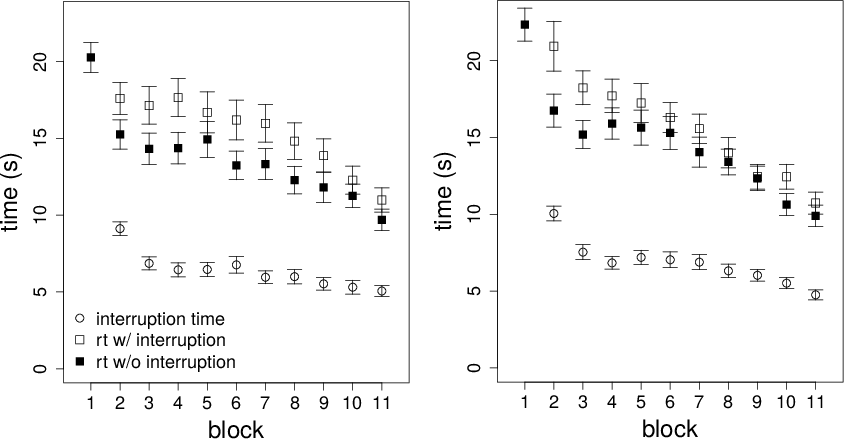
Participants were then free to view the outcomes by using the mouse to click in the empty grid cells. The outcome in that cell remained visible while the mouse button was depressed and was removed from view when the mouse button was released. Requiring the button to be depressed is a slight departure from some paradigms in which the cell is opened by moving the mouse into the box (e.g., Payne, et al, 1988). The current procedure was used to avoid inadvertently viewing a cell as the mouse is moved across the matrix. An alternative was selected by clicking on an alternative label. Participants had to view at least one outcome before selecting an alternative.
After an alternative was selected, one of the alternative outcomes was randomly sampled based on the outcome probabilities. The sampled outcome was added to the participant’s winnings. The participant was playing against the computer. Unknown to the participant, the computer picked the alternative with the highest expected value that had not been selected by the participant. The sampled outcome from the computer’s choice was added to the computer’s winnings. At the end of the experiment, participants needed to have won more money than the computer to qualify for the raffle.
On half of the trials in a block, the interruption trials, the participant was asked to complete an interruption task. The timing of the interruption within the trial is described in the Design section. There was a 1 second ‘pausing this decision’ warning, 6 seconds of the interruption task, and a 1 second ‘continuing previous decision’ message, for an 8 second total interruption. The length of disruption is in line with previous research (Monk, Trafton & Boehm-Davis, 2008; Monk, Boehm-Davis, Mason & Trafton, 2004).
Conditions 1 and 2 used different interruption tasks, but were otherwise identical. Condition 1 used a multiplication task. Two numbers, randomly sampled from 2 to 12, were shown multiplied on the screen along with a potential answer. Participants were asked to click ’true’ if the answer was correct and ’false’ otherwise. Half of the multiplications were correct. When false, the displayed incorrect answer was randomly selected to be within 2 of the correct answer. Condition 2 used a rotated-R task (e.g., Ratwani & Trafton, 2008). The letter R was shown on the screen rotated at a random angle from 0° to 340°in 20° increments. Half of the Rs were shown normally, the other half were shown mirror reversed. The participants were asked to click a button to indicate if the R was shown normally or mirror reversed.
Once one interruption task was complete, another started immediately. This process continued for 6 seconds. Participants were told that they needed to complete an average of 2 tasks per interruption to qualify for the bonus. After the interruption, the same, pre-interruption grid, with the same alternatives, probabilities, and outcomes in the same order, was provided to the participants, and the trial continued without further interruption until an alternative was selected. Participants were informed that the pre- and post-interruption grids were identical.
Experiment trials from all participants were included in all analyses. Only trials on which there were at least 2 pre-interruption and 2 post-interruption clicks were included. In Conditions 1 and 2, 1174 (28% of 4200) and 1637 (31% of 5340) trials were excluded from analysis, respectively. Most of these trials (88% and 90% of the excluded trials, respectively) were excluded because an alternative was selected before the interruption time or 1 click after the interruption time (which would prevent computation of some of the process measures). The proportion of excluded trials were very similar on the interruption and non-interruption trials (26% vs. 31% in Condition 1 and 31% vs. 31% in Condition 2). These data suggest that future research should consider using an earlier cutoff. As will become apparent, however, the remaining data provide a very clear, consistent pattern. In Conditions 1 and 2, 72 (2%) and 85 (2%) trials with a reaction time 3 or more standard deviations from the participant’s mean reaction time were removed from analyses, respectively.
On interruption trials in Conditions 1 and 2, participants completed an average of 2.16 (93% correct) and 2.08 (81% correct) interruption tasks per trial, respectively.
All analyses were performed in R 3.2.4 (R Core Team, 2016). Linear mixed effects models were performed using lme4 (Bates, Maechler, Bolker & Walker, 2015) and lmerTest for computation of p-values (Kuznetsova, Brockhoff & Christensen, 2016). The Bayesian analyses were performed using the BayesFactor package 0.9.12-2 (Morey & Rouder, 2015) using the default settings. In general, the conclusions of both analyses agreed (i.e., the ANOVA was significant when the Bayes factor was greater then 1 and not significant when the Bayes factor was less than 1). Tests on which they disagreed will be highlighted.
Before moving on to the measures discussed previously, consider overall reaction times. Figure 2 shows mean interruption time and mean reaction time as a function of interruption condition. Reaction time was measured from when the participant was free to click on the outcomes to when the participant selected a gamble. Recall that there were no interruption trials in the first block. A linear mixed effects model on reaction times was run with block (excluding the practice block), interruption (interrupted or not), and their interaction as fixed effects and random intercepts per participant. Participants sped up over time. There was an effect of block in both Condition 1, β=–1.63, SE=0.21, t=7.75, p<.001, and Condition 2, β=–2.08, SE=0.21, t=9.79, p<.001. Interruption trials were longer. There was an effect of interruption in both Condition 1, β=2.28, SE=0.30, t=7.66, p<.001, and Condition 2, β=1.66, SE=0.30, t=5.51, p<.001. There was a significant block-by-interruption interaction in Condition 2, β=–0.87, SE=0.30, t=2.90, p=.004, but not Condition 1, β=–0.45, SE=0.30, t=1.52, p=.13.
The details of the dependent variables are discussed next followed by the analyses.
This measure is the total number of outcome cells viewed by the participant. A view is a mouse click on an outcome cell. Repeated grid cells are counted as separate views, so there is no theoretical upper bound to this measure. The total number of cells viewed is a measure of how much information is gathered before a decision.
This measure is identical to the total number of cells viewed, but a view on each cell is only counted once. Because there are 16 outcome cells, the maximum value of this measure is 16. The number of unique cells viewed is a measure of how much distinctive information is gathered before a decision.
This measure is the total number of alternatives, or gambles, viewed. Viewing any outcome for an alternative counts as viewing the alternative. Repeated views for an alternative are only counted once. Because there are 4 alternatives, the maximum value of this measure is 4. The number of unique alternatives viewed is a measure of how much distinctive information is gathered before a decision. This measure is also of interest because participants may narrow down alternatives and focus on favorable gambles later in a trial (e.g., Payne, 1976). Thus, we might expect a reduction in unique alternatives viewed later in a trial.
This measure is the amount of time the participant views an outcome. The time to acquire information has been associated with decision-making effort (Payne, et al. 1988).
In the eye tracking literature, the processing of information can continue after the information is no longer visible, however, the eyes tend to stay in the same location until the processing is complete (e.g., Rayner, Liversedge, White & Vergilino-Perez, 2003). In the mouse-click paradigm, participants can view the contents of a cell for a short period of time (about 150ms below), but continue to process the information that was shown. As an analog to the eye tracking paradigm, we measure the time from when a cell was viewed until the next cell was viewed. The time between cells is a measure of effort and includes the time it takes to process the current cell and plan the next cell to view.
The Payne Index is a measure of the pattern of information acquisition (Payne, 1976; for caveats regarding the Payne Index, see Böckenholt & Hynan, 1994). Two potential information-gathering strategies are alternative- and attribute-based processing. In an alternative-based strategy, the participant views different attributes within a single alternative before moving to another alternative. Alternative-based processing is a hallmark of compensatory strategies (Payne, Bettman & Johnson, 1988). In attribute-based processing, the participant views a single attribute across different alternatives before moving to another attribute. Attribute-based processing is a hallmark of non-compensatory strategies (Payne, Bettman & Johnson, 1988) and is less cognitively effortful (Payne, Bettman & Johnson, 1993).
The Payne Index is defined here as
PI = (alternative count – attribute count) / (alternative count +
attribute count)
where alternative and attribute counts are the number of within-alternative and within-attribute mouse-clicks, respectively. For example, clicking on $43 (row 2, column 2) and then $72 (row 2 column 3) of Figure 1 is a within-alternative mouse-click. Clicking on $43 (row 2, column 2) and then $61 (row 3, column 2) is a within-attribute mouse click. Clicks that cross both alternatives and attributes were discarded. This measure ranges from –1 to +1, where a more positive value is indicative of alternative-based processing and a more negative value is indicative of attribute-based processing.
We also considered the first cell viewed at the beginning of a trial and the first cell viewed after the interruption-time. As will be discussed in more detail below, this variable will be used to measure the similarity of processing at the start of a trial and processing after the interruption-time.
Figure 3: Number of cells viewed on interruption and non-interruption trials before and after the interruption time for Conditions 1 (left panel) and 2 (right panel). Error bars are standard errors. 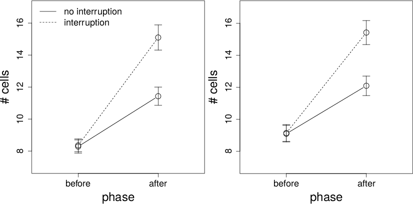
Table 1: Analysis of variance results for the process dependent measures of Conditions 1 and 2. Ph=Phase; Int=Interruption.
Condition 1 Condition 2 Variable F(1, 69) p F(1, 88) p Num cells Phase 181.30 <.001 224.10 <.001 Interruption 56.42 <.001 113.60 <.001 Ph × Int 67.52 <.001 101.50 <.001 Num unique cells Phase 183.60 <.001 155.90 <.001 Interruption 79.73 <.001 110.80 <.001 Ph × Int 61.59 <.001 78.60 <.001 Num unique alts Phase 0.20 0.66 11.21 0.001 Interruption 58.99 <.001 83.11 <.001 Ph × Int 77.62 <.001 74.39 <.001 Time per cell Phase 19.96 <.001 32.58 <.001 Interruption 0.23 0.64 1.10 0.30 Ph × Int 2.68 0.11 0.225 0.64 Time btw cells Phase 2.031 0.16 5.16 0.03 Interruption 17.24 <.001 24.03 <.001 Ph × Int 26.42 <.001 19.57 <.001 Payne Index Phase 48.12 <.001 74.16 <.001 Interruption 0.119 0.73 15.01 <.001 Ph × Int 0.464 0.498 15.51 <.001
Each gamble is associated with a payout. We measure the average amount won by the participant across trials. This is a measure of overall performance.
Table 2: Bayes factors for each nested model, relative to the subject-only model, for each process dependent measure of Conditions 1 and 2.
Dependent measure Model Num cells Num unique cells Num unique alts Time per cell Time btw cells Payne Index Condition 1 Phase 3.81E+30 6.10E+29 0.15 4.76E+07 0.35 1.19E+16 Int 247.20 712.94 4.10E+05 0.13 290 0.13 Ph + Int 4.14E+36 5.19E+36 6.35E+04 6.22E+06 110 1.60E+15 Ph × Int 1.91E+43 1.80E+44 1.42E+09 1.65E+06 1.06E+05 3.28E+14 Condition 2 Phase 5.35E+4 2.11E+34 197 1.20E+10 2.45 3.84E+25 Int 1430 1170 1.94E+06 0.16 723 0.68 Ph + Int 1.09E+51 1.20E+41 1.08E+09 1.97E+09 2920 7.80E+25 Ph × Int 3.34E+60 1.58E+49 3.79E+16 3.36E+08 3.62E+05 1.61E+26 Notes: Ph=Phase; Int=Interruption. Values greater than 10,000 are expressed in scientific format. The Ph × Int model includes both the interaction and main effect terms.
Because the gamble outcome is randomly determined, the average amount won is probabilistic. A more stable measure would look at how well the participant chose on every trial, regardless of the gamble outcome. On every trial, we calculated the expected value of each gamble. We then took the difference of the maximum expected value on that trial and the expected value of the participant’s selected gamble. We refer to this difference as the relative expected value. An average value of 0 means the participant selected the best alternative on all trials. The more negative the value, the poorer the participant’s choices.
For the first set of analyses, within each condition, both a within-subject ANOVA and a Bayesian analysis with phase (before or after the interruption time) and interruption (interruption or non-interruption trial) as within-subject factors and subject as a between-subject factor were performed. With the exception of first cell viewed, which will be analyzed separately, each of the process measures were used as dependent variables. Importantly, on the non-interruption trials, phase is determined by the time at which an interruption would have occurred had it been an interruption trial. Recall that all trials within a block have the same interruption time. Assume, for example, that the interruption time for a block is 6 seconds. Then any activity in the first 6 seconds of a trial will be placed into the before-interruption phase, regardless of trial type (i.e., interruption or non-interruption). All other activity (excluding the interruption task) is considered part of the after-interruption phase. The ANOVA results are provided in Table 1. The Bayes factors are provided in Table 2.
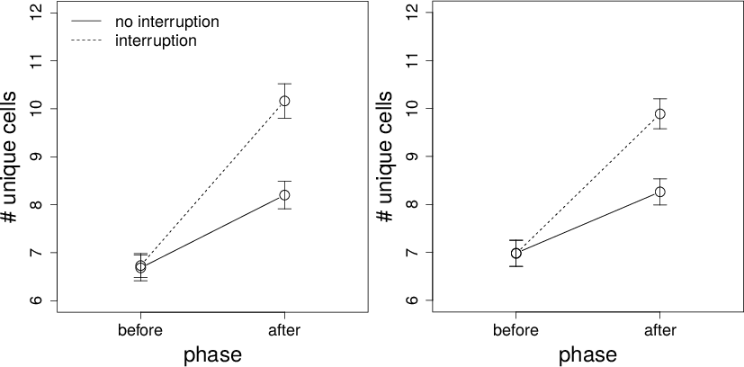
Figure 4: Number of unique cells viewed on interruption and non-interruption trials before and after the interruption time for Conditions 1 (left panel) and 2 (right panel). Error bars are standard errors.
The data for number of cells are shown in Figure 3. In both conditions, there were more viewed cells after an interruption, more viewed cells during an interruption trial, and an interruption-by-phase interaction. Importantly, the number of cells viewed after an interruption is significantly less (95% CI: 7.53-9.14 and 8.08-10.14 in Conditions 1 and 2, respectively) than the total number of cells viewed during an entire non-interruption trial, both in Condition 1, t(69)=20.66, p<.001, bf=1.00+E28, and in Condition 2, t(88)=17.63, p<.001, bf=2.39+E27. The idea is that, if, after an interruption, people started to processes the information from scratch, the number of cells viewed after an interruption would be the same as the total number of cells viewed during a non-interruption trial. After an interruption, fewer cells were viewed, suggesting that participants did not simply start the trial over.
The data for number of unique cells are shown in Figure 4. The results are qualitatively identical to the number of cells viewed. In both conditions, there were more viewed cells after an interruption, more viewed cells during an interruption trial, and an interruption-by-phase interaction. Again, participants viewed more unique cells (95% CI: 2.61–3.26 and 2.67–3.25 in Conditions 1 and 2, respectively) during a non-interruption trial than during the after phase of an interruption trial, both in Condition 1, t(69)=17.79, p<.001, bf=1.95+E24, and in Condition 2, t(88)=20.26, p<.001, bf=3.94+E31.
Figure 5: Number of unique alternatives viewed on interruption and non-interruption trials before and after the interruption time for Conditions 1 (left panel) and 2 (right panel). Error bars are standard errors.
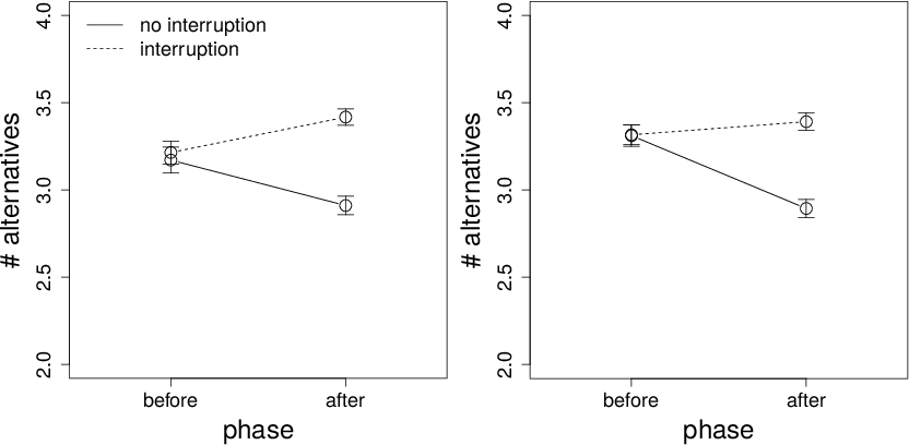
Figure 6: Viewing time per cell (ms) on interruption and non-interruption trials before and after the interruption time for Conditions 1 (left panel) and 2 (right panel). Error bars are standard errors.
The data for the number of unique alternatives are shown in Figure 5. In both conditions, there were more alternatives viewed after an interruption and a phase-by-interruption interaction. In Condition 2, but not Condition 1, there was also a significant effect of phase, such that there were fewer alternatives viewed after an interruption. Again, participants viewed more unique alternatives (95% CI: 0.71-0.87 and 0.72-0.88 in Conditions 1 and 2, respectively) during a non-interruption trial than during the after phase of an interruption trial, both in Condition 1, t(69)=18.95, p<.001, bf=6.76+E25, and in Condition 2, t(88)=20.94, p<.001, bf=4.15+E32.
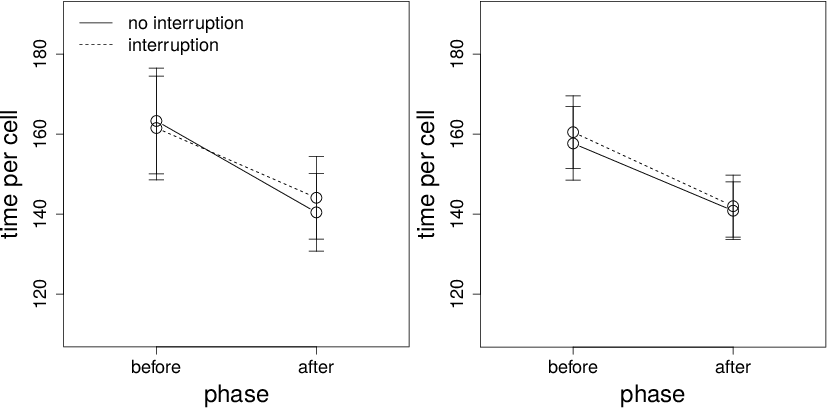
The data for time per cell are shown in Figure 6. Participants spent less time per cell later in a trial, i.e., after an interruption, but there was no effect of trial type and no interaction.
Figure 7: Top panels: Time between cell views (ms) on interruption and non-interruption trials before and after the interruption time for Conditions 1 (left panel) and 2 (right panel). Bottom panels: Time between cell views (ms) on interruption and non-interruption trials before the interruption time and for the first 5 cell views after the interruption time for Conditions 1 (left panel) and 2 (right panel). Error bars are standard errors.
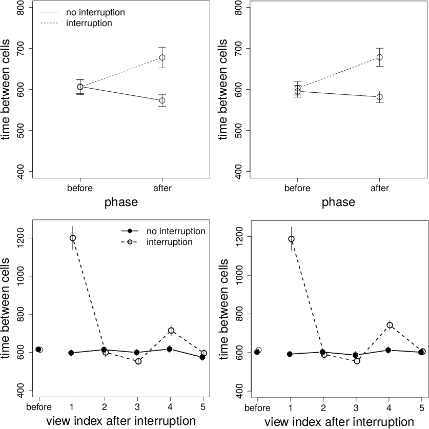
The data for time between cells are shown in the top panels of Figure 7. There is a significant effect of trial type and a phase-by-interruption interaction. Participants spent more time after an interruption. Importantly, however, the interaction is mainly caused by the cell views immediately after the interruption. These data are shown in the bottom panels of Figure 7. The leftmost points are the mean time between cells before the interruption time. The remaining points are the mean between cell times for the first five outcome views after the interruption. As the sample size for each data point can vary greatly (i.e., the number of data points necessarily decreases over time and participants contributed differentially to each point), these data should be taken as a rough estimate. That said, the result seems clear: There is a substantial increase in time immediately after an interruption, which rapidly disappears. This result suggests a strong, short-lived processing cost of interruption. The ANOVA also produces a significant effect of phase for Condition 2. The Bayes factor for this effect, however, is small.
Figure 8: Payne Index on interruption and non-interruption trials before and after the interruption time for Conditions 1 (left panel) and 2 (right panel). Error bars are standard errors.
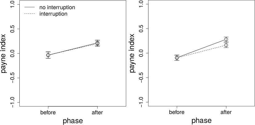
The Payne Index data are shown in Figure 8. There is little to no preference for alternative- or attribute-wise processing before the interruption time. After the interruption time, however, there is a preference for alternative-wise processing. As discussed previously, this result suggests a preference for compensatory strategies later in a trial. There is no hint of a phase-by-interruption interaction in Condition 1. In Condition 2, the ANOVA shows a significant effect of interruption and a significant phase-by-interruption interaction. These latter results should be accepted with caution. The Bayes factor for the interaction is about 21, suggesting only very weak evidence in favor of the interaction. Thus, more evidence is needed before concluding that the interaction is real.
Figure 9: Heatmap of the first cell viewed at the beginning of a trial, immediately before the interruption time, and immediately after the interruption time on interruption and non-interruption trials for Conditions 1 (top 6 panels) and 2 (bottom 6 panels). Lighter colors indicate higher proportions. 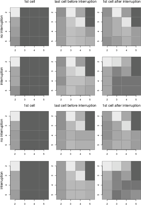
The first cell viewed data was analyzed differently. These data are shown in Figure 9. Each panel represents the 16 outcome cells as arrayed on the screen. The cells are numbered from 2 to 5 to be consistent with the stimuli description above in which the outcome cells started at Row and Column 2. The brightness of a cell indicates the proportion of times a cell is viewed either as the first cell of the trial (left column), the last cell before the interruption time (center column), or the first cell after the interruption time (right column) on interruption and non-interruption trials. Lighter colors indicate higher proportions. Data from Conditions 1 and 2 are shown in the top and bottom 6 panels, respectively.
Consider the first cell viewed during a trial. Regardless of trial type or condition, participants overwhelmingly looked at the left column and, in particular, the top-left cell (Row 2, Column 2). This result is interesting by itself. Recall that the probabilities associated with each column vary and are randomly ordered. This result suggests that physical ordering was more important to participants than the probability of an outcome, at least for the first cell viewed.
Figure 10: Average amount won (left panels) and relative expected value (right panels) on interruption and non-interruption trials in Conditions 1 (top panels) and 2 (bottom panels). 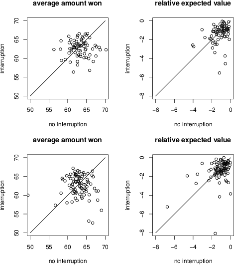
Next, consider the first cell viewed after the interruption time. A consistent pattern emerges. On non-interruption trials, viewing is relatively egalitarian, with Cells (2, 3) and (3, 4) particularly favored. Note that Cell (2, 2), the initially favored top left cell, has a relatively low proportion of views. On interruption trials, however, the pattern is somewhat different. The bottom right area has fewer views. Cells (2, 3) and (3, 4) still have higher views than on the first cell viewed. Importantly, however, the proportion of views to the top left Cell (2, 2) is now high. To quantify this pattern, we correlated the cell-by-cell after-interruption viewing proportions on the interruption trials to (1) the after-interruption cell viewing proportions on the interruption trials and (2) the first cell viewing proportions on the interruption trials. In both conditions, the correlation in (2) was much higher than in (1), suggesting that participants, do, to some extent, restart their viewing pattern. For Condition 1, (1) r=.35, t(14)=1.39, p=.19 and (2) r=.71, t(14)=3.80, p=.002. For Condition 2, (1) r=.48, t(14)=2.03, p=.06 and (2) r=.70, t(14)=3.65, p=.003. Note, however, that, although the correlation is lower, there is also considerable overlap with the post-interruption viewing pattern. Overall, the viewing pattern after an interruption is consistent with a mixture of both starting the trial over and continuing the trial.
The last cell viewed before the interruption time was included as a comparison. Note that, because the interruption has not yet taken place, the pattern for the interruption and non-interruption trials is qualitatively identical. Because they are only one click apart, the pattern for the last cell before the interruption time and first cell after the interruption time on non-interruption trials are also identical. As expected, however, the patterns are different on interruption trials and, as discussed previously, are consistent with a mixture of both restarting and continuing the trial.
The analyses up to this point have focused on how processing measures change as a function of phase and interruption. The next set of analyses are more global – they ask whether overall performance in the task is harmed by the presence of an interruption. In particular, the question is how well participants did at selecting alternatives on interruption and non-interruption trials.
The left panels of Figure 10 show the mean total amount won on interruption and non-interruption trials for each participant in each condition. Points above and below the line indicate more won on interruption and non-interruption trials, respectively, for each participant. There was no overall difference between interruption and non-interruption trials in either Condition 1, t(69)=1.41, p=.16, bf=0.34, or Condition 2, t(88)=1.17, p=.24, bf=0.23.
The relative expected value data are shown in the right panels of Figure 10. Recall that the best a participant can do is 0, indicating an optimal choice on every trial. More negative values are worse performance. Points above and below the line indicate better performance on interruption and non-interruption trials, respectively. With few exceptions, participants selected alternatives relatively well. There was, however, no overall difference between interruption and non-interruption trials in either Condition 1, t(69)=1.53, p=.13, bf=0.39, or Condition 2, t(88)=1.08, p=.28, bf=0.20.
This research examined the effect of interruptions on cognitive processing during a risky decision-making task. The research had two main goals: first, to extend our knowledge of the effect of interruptions to a commonly used risky decision-making task; and second, more importantly, to determine the effect of interruptions on the information gathering process. Participants were asked to choose among a set of 4 gambles. Each gamble had 4 outcomes. Each outcome was associated with a probability of occurrence. To view an outcome, participants had to use the mouse to click on the location of the outcome in a grid. On half of the trials, participants were interrupted with a secondary task, either a multiplication or spatial task. The viewing locations, order, and times were used to determine general parameters of the processing strategies used by participants during the task.
Although there is evidence that the relationship between the main task and interruption task can differentially affect processing disruption (Gillie & Broadbent, 1989), across all measures, both the qualitative and quantitative results from Conditions 1 and 2 were extremely similar. It is too early to say whether, in this decision-making task, the two types of interruptions affected the same processes or different processes with the same outcome. Regardless, in most of what follows we discuss the two interruption tasks together.
Consistent with past work, interruptions did come with a cost. Compared to the same time period during non-interruption trials, after an interruption, participants sampled more cells, more unique cells, and more alternatives. But there was also a relative savings. After an interruption, these measures were less than during the whole of a non-interruption trial. If participants had completely started the trial over, the after-interruption and non-interruption measures would be the same.
A similar savings was found in a reading study (Cane, Cauchard & Weger, 2012) in which participants did not have to completely re-read a passage after an interruption. This result was attributed to long-term working memory theory (Ericsson & Kintsch, 1995) and, in particular, to the idea that particpants were able to encode some of the pre-interruption information into memory. We advocate a similar, simple explanation here: participants retained some memory of the pre-interruption gamble outcomes after the interruption.
These data do not adjudicate between extent models of interruption. Indeed, a number of interruption theories, including memory for goals (Altmann & Trafton, 2002; Monk, Trafton & Boehm-Davis, 2008) and prospective memory theory (Boehm-Davis & Remington, 2009; Dismukes, 2010; Dodhia & Dismukes, 2009; Einstein, McDaniel, Williford & Dismukes, 2003), incorporate similar memory-based mechanisms. Memory for goals, for example, suggests that, during the interruption warning, participants encode the to-be-remembered information in memory and then use task cues to aid in the retrieval of this information after the interruption. Despite the use of a short, 1-second interruption warning and no explicit recovery cues upon return to the main task, participants in the current task were able to complete the trial without completely starting over. Although explicit recover cues were not present, neither the grid nor task changed post-interruption. Previous work has suggested that if the structure of the problem maintains consistency pre- and post-interruption, participants are able to maintain a memory representation of the information which lessens the interruption effect (Edwards & Gronlund, 1998).
Although the time spent directly viewing each outcome did not change after an interruption (Gillie & Broadbent, 1983), presumably because only a fixed amount of viewing time is needed to encode the outcome, participants did spend more time between outcome views immediately after an interruption. This result is consistent with both the task-switching literature, which has found that there is a large cost associated with switching between tasks (e.g., Monsell, 2003), and the standard finding of a resumption lag after an interruption (e.g., Altmann & Trafton, 2004; Altmann & Trafton, 2007; Monk, Trafton & Boehm-Davis, 2008; Trafton, Altmann, Brock & Mintz, 2003). For example, using a computer game as the main task, Altmann and Trafton (2007) found that response times more than doubled after an interruption and this disruption was almost gone approximately 3 trials after the interruption.
The data strongly suggest that an interruption did cause participants to, at least partially, restart the trial. In addition to the increased information gathering after an interruption discussed previously, the pattern of first cell views after an interruption were more similar to the first cell view of a trial than to a similarly timed cell view that did not follow an interruption. Previous research has suggested that individuals who lose their place in a task have a tendency to start over (Ratwani & Trafton, 2008). Furthermore, some research suggests that spatial memory is especially prone to disruption by an interruption (Trafton, Altmann & Ratwani, 2011). Inspection of Figure 9, however, supports a mixture of the two strategies, suggesting that, for some participants or on some trials, the information search pattern after an interruption continued as if an interruption had not occurred. Although our current data do not speak to this question, an interesting avenue for future research would be to continue pursuing the factors that lead to these different strategies. It is worth noting that, although the rotated-R task was expected to have a more disruptive effect on spatial memory, the pattern of first cell views was very similar across conditions.
It is possible that participants reduced their effort after an interruption, perhaps due to fatigue, leading to a change in these processing measures. While possible, overall performance was not affected, as might be expected if effort was decreased. Indeed, overall performance measures were nearly identical on interruption and non-interruption trials. This result is surprising. It suggests that, in this task, although there is a cost to an interruption in terms of time and effort, participants were able to completely overcome the disruption.
Indeed, there is evidence that the interruption did not change the information gathering strategy of the participants. In particular, the Payne Index, a measure of processing strategy, was very similar regardless of whether or not an interruption occurred. Early in the trial, participants showed little preference for alternative- or attribute-wise search. Later in the trial, however, an alternative-wise strategy was slightly favored on all trials. Coupled with the reduction in unique alternatives viewed later in a trial on non-interruption trials, this pattern is consistent with the idea that participants narrowed down the set of alternatives early in the trial and then examined attributes within alternatives later in the trial. We note that a return to early processing strategies after an interruption would tend to push the Payne Index more towards pre-interruption levels, as was seen in the tentative interaction of Condition 2. Under that explanation, however, it is the lack of an interaction in Condition 1 that deserves further thought. Full consideration of this issue is left for future research.
The nature and effect of interruption on task performance is well-explored. Most results suggest that these effects are negative. The impact of the interruption on the processing strategy, however, is seldom considered. This research was a step towards addressing that gap in a common decision-making paradigm. Regarding performance measures, an interruption affected this decision-making task as expected and consistent with past work. In particular, an interruption increased the processing effort and time. Somewhat surprisingly, however, no decrement was seen in performance. Regarding processing strategy, the interruption caused participants to partially restart the task, but otherwise approach the task in the same fashion. Because interruptions have caused large disruptions in performance in past studies (e.g., Altmann, Trafton & Hambrick, 2013; Gillie & Broadbent, 1989; Trafton, Altmann, Brock & Minz, 2003), this result is somewhat surprising and is further evidence that the effect of an interruption is based, in part, on the task being interrupted. The data imply a simple explanation: a subset of pre-interruption information was recalled, which was then incorporated into post-interruption processing.
Although simple and intuitive, this explanation is potentially informative in a number of ways. These data help inform formal models of interruption. For example, they provide constraints on the retention and later recall of pre-interruption information. How much and which information is retained and how retention interacts with the task environment are important open questions (but see Edwards & Gronlund, 1998). The data also indicate a significant, but short-lived interruption effect with considerable variability across trials and/or participants. More importantly, the lack of a change in processing is in itself interesting and counterintuitive. That is, previous research has suggested that processing strategies may change during the course of a trial or after an interruption. For example, decision makers have been observed to change strategies as a result of task characteristics such as problem complexity or managing time pressures (Payne, 1976; Zur & Breznitz, 1981). Taken together, these results are moderately encouraging for the effect of interruptions on processing in decision-making tasks. Interruptions do delay processing and increase effort. This delay can cause problems in time-sensitive tasks. Relative to non-interruption trials, however, participants don’t seem to resort to shortened or poorer processing after an interruption. As a consequence, overall performance does not decrease.
Altmann, E. M., & Gray, W. D. (2000). Managing attention by preparing to forget. In Human Factors and Ergonomics Society 44th Annual Meeting (pp. 152–155). Santa Monica, CA: Human Factors and Ergonomics Society.
Altmann, E. M. & Trafton, J.G. (2007). Timecourse of recovery from task interruption: Data and a model. Psychonomic Bulletin & Review, 14(6), 1079–1084.
Altmann, E. M. & Trafton, J. G. (2002). Memory for goals: An activation-based model. Cognitive Science, 26, 39–83.
Altmann E. M. & Trafton J. G. (2004) Task interruption: Resumption lag and the role of cues. In Proceedings of the 26th Annual Conference of the Cognitive Science Society (pp. 42–47). Hillsdale, NJ: Erlbaum.
Altmann, E. M., Trafton, J.G., & Hambrick, D. Z. (2013). Monentary interruptions can derail the train of thought. Journal of Experimental Psychology: General, 143(1), 215–226.
Bates, D., Maechler, M., Bolker, B., & Walker, S. (2015). Fitting linear mixed-effects models using lme4. Journal of Statistical Software, 67(1), 1–48. http://dx.doi.org/10.18637/jss.v067.i01.
Bailey, B. P. & Konstan, J. A. (2006). On the need for attention-aware systems: Measuring effects of interruption on task performance, error rate, and affective state. Computers in Human Behavior, 22(4), 685–708.
Böckenholt, U. & Hynan, L. S. (1994). Caveats on a process-tracing measure and a remedy. Journal of Behavioral Decision Making, 7(2), 103–117.
Boehm-Davis, D. A., & Remington, R. (2009). Reducing the distruptive effects of interruption: A cognitive framework for analysing the costs and benefits of intervention strategies. Accident Analysis and Prevention, 41(5), 1124-1129.
Brumby, D. P., Cox, A. L., Back, J., & Gould, S. J. (2013). Recovering from an interruption: Investigating speed-accuracy trade-offs in task resumption behavior. Journal of Experimental Psychology: Applied, 19(2), 95–107.
Cades, D. M., Davis, D. A. B., Trafton, J. G., & Monk, C. A. (2007). Does the Difficulty of an Interruption Affect our Ability to Resume? In Proceedings of the 51st Annual Meeting of the Human Factors and Ergonomics Society (pp. 234–238). Santa Monica, CA: Human Factors and Ergonomic Society.
Cane, J. E., Cauchard, F., & Weger, U. W. (2012). The time-course of recovery from interruption during reading: Eye movement evidence for the role of interruption lag and spatial memory. The Quarterly Journal of Experimental Psychology, 65(7), 1397–1413.
Czerwinski, M., Cutrell, E., & Horvitz, E. (2000). Instant messaging: Effects of relevance and timing. In People and computers XIV: Proceedings of HCI (pp. 71–76). London: British Computer Society.
Diez, M., Boehm-Davis, D. A., & Holt, R. W. (2002). Model-based predictions of interrupted checklists. In Proceedings of the 46th Annual Meeting of the Human Factors and Ergonomics Society (pp. 250–254). Santa Monica, CA: Human Factors and Ergonomics Society.
Dismukes, R. K. (2010). Remembrance of things future: Prospective memory in laboratory, workplace, and everyday settings. Reviews of Human Factors and Ergonomics, 6(1), 79–122.
Dodhia, R. M. & Dismukes, R. K. (2009). Interruptions create prospective memory tasks. Applied Cognitive Psychology, 23(1), 73–89.
Edwards, M. B. & Gronlund, S. D. (1998). Task interruption and its effects on memory. Memory, 6(6), 665–687.
Edwards, W., Lindman, H., & Savage, L. J. (1963). Bayesian statistical inference for psychological research. Psychological Review, 70(3), 193-242.
Einstein, G. O., McDaniel, M. A., Williford, C. L., & Dismukes, R. K. (2003). Forgetting of intentions in demanding situations is rapid. Journal of Experimental Psychology: Applied, 9(3), 147–162.
Ericsson, K. A. & Kintsch, W. (1995). Long-term working memory. Psychological Review, 102(2), 211–245.
Gallistel, C. (2009). The importance of proving the null. Psychological Review, 116, 439–453.
Gillie, T. & Broadbent, D. (1989). What makes interruptions disruptive? A study of length, similarity, and complexity. Psychological Research, 50, 243–250.
Grundgeiger, T. & Sanderson, P. (2009). Interruptions in healthcare: Theoretical views. International Journal of Medical Informatics, 78(5), 293–307.
Grundgeiger, T., Liu, D., Sanderson, P. M., Jenkins, S., & Leane, T. (2008). Effects of interruptions on prospective memory performance in anesthesiology. In Proceedings of the 52nd Annual Meeting of the Human Factors and Ergonomics Society (pp. 808–812). Santa Monica, CA: Human Factors and Ergonomics Society.
Grundgeiger, T., Sanderson, P., MacDougall, H. G., & Venkatesh, B. (2010). Interruption management in the intensive care unit: Predicting resumption time and assessing distributed support. Journal of Experimental Psychology: Applied, 16(4), 317–334.
Hodgetts, H. M. & Jones, D. M. (2006). Contextual cues aid recovery from interruption: The role of associative activation. Journal of Experimental Psychology: Learning, Memory and Cognition, 32(5), 1120–1132.
Jeffreys, H. (1961). Theory of probability (3rd ed.). New York: Oxford University Press.
Kass, R. & Raftery, A. E. (1995). Bayes factors. Journal of the American Statistical Association, 90(430), 773–795.
Kuznetsova, A., Brockhoff, P., & Christensen R. (2016). lmerTest: Tests in linear mixed effects models. r package (Version 2.0-32) [Software]. Available from https://CRAN.R-project.org/package=lmerTest
Latorella, K. A. (1998). Effects of modality on interrupted flight deck performance: Implications for data link. In Proceedings of the 42nd Annual Meeting of the Human Factors and Ergonomics Society (pp. 87-91). Santa Monica: Human Factors and Ergonomics Society.
Li, S. Y., Blandford, A., Cairns, P., & Young, R. M. (2008). The effect of interruptions on postcompletion and other procedural errors: An account based on the activation-based goal memory model. Journal of Experimental Psychology: Applied, 14(4), 314-328.
Liu, W. (2008). Focusing on desirability: The effect of decision interruption and suspension on preferences. Journal of consumer research, 35, 640–652.
Liu, D., Grundgeiger, T., Sanderson, P., Jenkins, S., & Leane, T.A. (2009). Interruptions and blood transfusion checks: Lessons from simulated operating room. Anesthesia and Analgesia, 108(1), 219–222.
Miller, S. L. (2002). Window of opportunity: Using the interruption lag to manage disruption in complex tasks. In Proceedings of the 46th Annual Meeting of the Human Factors and Ergonomics Society (pp. 245–249). Santa Monica, CA: Human Factors and Ergonomic Society.
Monk, C. A., Boehm-Davis, D. A., Mason, G., & Trafton, J.G. (2004). Recovering from interruptions: Implications for driver distraction research. Human Factors, 46(4), 650–663.
Monk, C. A., Trafton, J. G., & Boehm-Davis, D. A. (2008). The effect of interruption duration and demand on resuming suspended goals. Journal of Experimental Psychology: Applied, 14(4), 299-313.
Monsell, S. (2003). Task switching. Trends in Cognitive Sciences, 7(3), 134–140.
Morey, R. & Rouder, J. N. (2015). Bayes factor: computation of bayes factors for common design. R package (Version 0.9.1201) [Software]. Available from https://CRAN.R-project.org/package=BayesFactor
Oulasvirta, A. & Saariluoma, P. (2006). Surviving task interruptions: Investigating the implications of long-term working memory theory. International Journal of Human-Computer Studies, 64, 941–961.
Payne, J. W. (1976). Task complexity and contingent processing in decision making: An information search and protocol analysis. Organizational Behavior and Human Performance, 16, 366-387.
Payne, J. W., Bettman, J. R., & Johnson, E. J. (1993). The Adaptive Decision Maker. Cambridge: University Press.
Payne, J. W., Bettman, J. R., & Johnson, E. J. (1988). Adaptive strategy selection in decision making. Journal of Experimental Psychology: Learning, Memory, and Cognition, 14(3), 534–552.
R Core Team. (2016). R: A language and environment for statistical computing. R Foundation for Statistical Computing [Software]. Available from https://www.R-project.org/
Ratwani, R. & Trafton, J. G. (2008). Spatial memory guides task resumption. Visual Cognition, 16(8), 1001–1010.
Ratwani, R. & Trafton, J.G. (2010). An eye movement analysis of the effect of interruption modality on primary task resumption. Human Factors, 52(3), 370–380.
Rayner, K., Liversedge, S. P., White, S. J., & Vergilino-Perez, D. (2003). Reading disappearing text cognitive control of eye movements. Psychological Science, 14(4), 385–388.
Rouder, J., Speckman, P. L., Sun, D., Morey, R. D., & Iverson, G. (2009). Bayesian t-tests for accepting and rejecting the null hyplthesis. Psychonomic Bulletin & Review, 16, 225–237.
Speier, C., Valacich, J. S., & Vessey, I. (1999). The influence of task interruption on individual decision making: An information overload perspective. Decision Sciences, 30(2), 337–360.
Speier, C., Vessey, I., & Valacich, J. S. (2003). The effects of interrputions, task complexity, and information presentation on computer-supported decision-making performance. Decision Sciences, 34(4), 771–797.
Trafton, J. G. & Monk, C. A. (2008). Task interruptions. In D. Boehm-Davis (Ed.), Reviews of Human Factors and Ergonomics (pp. 111-126). Santa Monica: Human Factors and Ergonomics Society.
Trafton, J. G., Altmann, E. M., & Ratwani, R. M. (2011). A memory for goals model of sequence errors. Cognitive Systems Research, 12(2), 134–143.
Trafton, J. G., Altmann, E. M., Brock, D. P., & Mintz, F. E. (2003). Preparing to resume an interrupted task: Effects of prospective goal encoding and retrospective rehearsal. International Journal of Human-Computer Studies, 58(5), 583–603.
Wagenmaker, E. (2007). A practical solution to the pervasive problem of p values. Psychonomic Bulletin and Review, 14, 779–804.
Zeigarnik, B. (1938). On finished and unfinished tasks. In W. D. Ellis (Ed.), A Source Book of Gestalt Psychology (pp. 300–314). London: Routledge.
Zur, H. B. & Breznitz, S. J. (1981). The effect of time pressure on risky choice behavior. Acta Psychologica, 47(2), 89–104.
We thank Meaghan Valler for suggesting the interruption task for Condition 2 and her help with running participants.
Copyright: © 2016. The authors license this article under the terms of the Creative Commons Attribution 3.0 License.
This document was translated from LATEX by HEVEA.