Judgment and Decision Making, Vol. 12, No. 2, March 2017, pp. 118-127
Hold on to it? An experimental analysis of the disposition effectMatteo Ploner* |
This paper experimentally investigates a well-known anomaly in portfolio management, i.e., the fact that paper losses are realized less than paper gains (disposition effect). I confirm the existence of the disposition effect in a simple risky task in which choices are taken sequentially. However, when choices are planned ahead and a contingent plan is defined, a reversal in the disposition effect is observed.
Keywords: decision making under uncertainty, disposition effect, behavioral finance, experiments
The disposition effect is one of the most investigated anomalies in financial markets, since the pioneering contribution of Shefrin and Statman (1985). The term identifies an asymmetry in liquidation patterns according to which individuals who experienced a loss in an investment are more likely to hold on to it compared to individuals who experienced a gain. The phenomenon has important implications both for individual portfolio management and for aggregate market dynamics (Coval & Shumway, 2005).1
I exploit the advantages of a laboratory experiment to further our understanding of the disposition effect and to assess how alternative decision making protocols may affect it. Subjects in the experiment face a series of choices over simple risky prospects. To assess the existence of a disposition effect, I compare the decision to take part in a risky investment of those who had experienced a loss and those who had experienced a gain, in a prior risky choice. In one condition, subjects define a contingency plan to deal with a loss or a gain before knowing the actual outcome of the first risky choice (strategy method); in another condition, subjects choose immediately after knowing the outcome of the first risky choice (direct response). The two choice protocols have equivalent results but are likely to differ in terms of emotional involvement: the strategy method is usually described as “colder” than the direct response method (see, among others, Brandts & Charness, 2000).
The present study documents the existence of a disposition effect in the direct response choice protocol and shows that this is mainly due to the reluctance to realize losses. However, when choices are taken via the strategy method, a reverse disposition effect is observed, with losers less likely to hold on to their investment than winners. Overall, I observe that the behavior of losers is affected more by previous events and by elicitation methods than that of winners. Furthermore, the collected evidence suggests that the liquidation patterns emerging in the experiment are not likely to originate in wealth effects or in idiosyncratic beliefs about stochastic realizations but in asymmetric risk preferences of winners and losers.
In sum, I find that alternative choice protocols, which are equivalent in terms of their consequences, may generate opposite effects of risk exposure. This result may help achieve a better understanding of a well-known anomaly in finance.
Since the seminal work of Shefrin and Statman (1985), the relevance of the disposition effect for financial markets has been highlighted by several empirical studies, both in the US (Odean, 1998) and in China (Chen, Kim, Nofsinger & Rui, 2007). Furthermore, the disposition effect seems to extend also to non-financial domains, like real estate markets (Genesove & Mayer, 2001) and job incentives (Heath, Huddart & Lang, 1999).
A combination of Prospect Theory (Kahneman and Tversky, 1979) and mental accounting (Thaler, 1999) provides the leading explanation for the emergence of the disposition effect (for an early account, see Shefrin & Statman, 1985). According to Prospect Theory, individuals do not evaluate the performance of an investment in terms of its utility consequences, but assess the performance in terms of its deviation from a given reference point (e.g., the purchase price). Moreover, individuals are risk seekers for negative deviations from the reference point (losses) and are risk averse for positive deviations (gains). From this, it follows that those who experience a gain are less likely to hold on to the risky investment than those who experience a loss.
Grinblatt and Han (2005) present a theoretical model with heterogeneous agents in which a fraction of the agents behaves as predicted by the disposition effect. An empirical estimation of the model provides support to the combination of Prospect Theory and mental accounting as the determinant of the drift in prices. In a similar vein, Frazzini (2006) shows that price predictability is higher when the disposition effect predicts more under-reaction to corporate news. A few works, however, questioned the relevance of Prospect Theory in explaining the disposition effect. Kaustia (2010) shows that the pattern of realized returns in field data cannot be captured by reasonable parameterizations of the model. Barberis and Xiong (2009) show that the emergence of the disposition effect is strictly linked to the assumption that individuals experience “a burst of utility right then, at the moment of sale”. Empirical support to this assumption comes from some recent experimental findings (Frydman et al., 2014; Frydman & Rangel, 2014).
Most of the tests of the disposition effect rely on field studies. Only a few attempts have been made to investigate the phenomenon experimentally. In a pioneering contribution, Weber and Camerer (1998) study behavior in a laboratory experiment replicating a portfolio management situation. Subjects buy and sell stocks over a series of rounds and need to infer the stochastic process underlying each artificial stock. The authors find that selling is more frequent when a stock rises in price than when it falls, which is in line with the disposition effect.
Weber and Zuchel (2005) investigate dynamic risky decisions in a two-stage experimental setting similar to the one employed here. However, the aim of the authors is not to compare alternative choice protocols, as they consider only choices collected via a contingent plan. The experimental manipulations performed by Weber and Zuchel refer to the presentation format of the investment, i.e., either as a portfolio management task or as a choice over lotteries, and to the freedom of choice, i.e., the choice in the first period is either made by the subject or by the experimenter. The authors report that the portfolio framework tends to generate results compatible with the disposition effect, with more risk taking behavior following a loss than following a gain. Differently, in the lottery condition no effects are observed in the free choice setting and a reverse disposition effect emerges in the condition in which the first choice is imposed by the experimenter.
In a recent contribution, Imas (2016) points out some conflicting results in the literature investigating dynamic decision-making. Some works document higher risk propensity after a loss (e.g., Langer & Weber, 2008), a result compatible with the disposition effect, while others find lower risk propensity after a loss (e.g., Shiv et al., 2005). The experimental evidence collected by Imas (2016) suggests that the realization of losses plays an important role in explaining divergent behavior in dynamic investment decisions. Specifically, when losses from an investment are cashed in, investors tend to lower their risk propensity. In contrast, when losses are “kept on the paper”, the risk propensity of investors increases after a loss.
Fischbacher, Hoffmann and Schudy (forthcoming) investigate whether the opportunity to commit to profit/losses realizations via automatic trading systems affects the disposition effect. The authors adopt a market setting similar to that of Weber and Camerer (1998) and find that, when subjects in the experiment can commit to sell stocks at a given limit price, the disposition effect tends to reverse. Interestingly, the trading system works when it automatically executes orders at the threshold price and not when it just delivers a signal that the threshold price was hit. Also one of the choice protocols investigated here implements a trading rule. However, the rule is defined directly on outcomes in the previous round of a perfectly known stock and not on hit prices of stocks whose underlying stochastic process has to be inferred over time. In addition, the setting adopted here offers a strict control about potential wealth effects and perfectly balances the likelihood of obtaining a gain and a loss across experimental conditions.
Subjects in the experiment make choices involving risky prospects. All prospects are simple win/loss gambles with the same probability assigned to the win and to the loss outcome. The loss outcome (l) is always equal to –40 Experimental Currency Units (ECU), while the win outcome (w) differs across prospects and can assume the following values: +20, +30, +40, +50, and +60 ECU. It follows that Prospects #1 and #2 have a negative expected value (EV), Prospect #3 is a fair prospect, and Prospects #4 and #5 have a positive expected value (see Table 1).
The experiment is composed of a main phase (Phase 1) and a control phase (Phase 2). In Phase 1, subjects are given an endowment E1=100 ECU and must choose whether to invest it in an asset X or in an asset Y. The subjects are aware that X warrants a win if the outcome of rolling a fair six-sided die is lower than 4, and a loss otherwise. The opposite holds for Y: when the outcome is higher than 3, returns are positive and when the outcome is lower than 4, returns are negative. The two assets are ex-ante identical and perfectly anti-correlated.2 As an example, consider Prospect #4 yielding 50 ECU for a win: if the subject chooses X and the outcome of the roll is 2, the subject earns E1+50 ECU.
After becoming aware of the outcome of the first roll, each subject chooses whether she wants to hold on to the investment or to sell it. When holding on, a second roll of the die is performed and earnings computed as in the first roll. When selling, the outcomes of the first roll are paid to the subject and the round ends. As an example, consider the prospect yielding 50 ECU when the outcome is favorable: if the outcome of the first roll is a win and the outcome of the second roll is a loss, earnings in the round are equal to E1+50−40. In Phase 1, the five risky prospects of Table 1 are implemented as independent investment choices over five distinct rounds.3 Given this setting, a straightforward measure of the disposition effect is obtained by comparing the relative frequency of hold choices (hold rate) among those winning and those losing after the first roll of the die.4
The investment choices in Phase 2 are also based on the same five risky prospects of Phase 1 (see Table 1), but involve only one roll of a fair die. Similarly to Phase 1, subjects choose whether to invest in X or in Y. However, in Phase 2 there is only one roll of the die and subjects can choose whether to take part in the gamble or not. In Phase 2, subjects choose twice for each prospect over 10 distinct rounds, with the initial endowment E2 differing in each round. The values of the initial endowments are defined to replicate the two possible outcomes of the first roll of the die in Phase 1. As an example, Prospect #2 is implemented twice, once with an endowment E2=120 ECU and once with endowment E2=60 ECU. The two endowments are obtained by adding to the starting endowment of 100 ECU the win amount (w=20) of Prospect #2 and the loss amount (l=–40) of Prospect #2, respectively. The same procedure is replicated for all prospects to obtain the 10 prospects of Phase 2.
Importantly, Phase 2 allows us to check for the impact of wealth effects on the choices of winners and losers. The aim of Phase 2 is to put subjects in the same economic condition of a winner or a loser, but to avoid the personal experience of the success/failure of the investment. When differences between losers and winner are motivated only by differences in accumulated wealth, the same pattern of behavior should be observed in Phase 1 and in Phase 2. The introduction of Phase 2 fills a gap in the literature; to the best of my knowledge, previous related studies do not provide an explicit control for wealth effects.
The experiment relies on two between-subjects treatments (see Table 2 for a summary).5
Table 2: Experimental conditions.
Endowment
The Choice Protocol treatment refers to the the procedure adopted to collect choices in Phase 1. In the Sequential condition, subjects choose whether to hold or to sell their investment, after becoming aware of the outcome of the first roll of the die (direct response). Specifically, in each round subjects go through the following sequence of events: first, subjects choose between the investment X and the investment Y; second, a roll of the die is performed to define the investment returns; third, subjects choose whether to hold or to sell the investment; fourth, a second roll of the die is performed to define the investment returns for those who chose to hold on to the investment; finally, all subjects obtain a summary about the returns of their investment. This sequence is repeated five times over five distinct rounds, with each prospect of Table 1 displayed only once to each subject.
In the Planned condition, in each round subjects go through the following sequence of events: first, they choose between the investment X and the investment Y; second, they define a contingent plan in which they state whether they want to hold or to sell the investment, conditional upon obtaining a win outcome or a loss outcome in the first roll. This contingent plan is binding and cannot be renegotiated after the outcome of the first roll (strategy method); third, two rolls of the die are performed in sequence to define the investment returns. The second roll of the die is relevant only for those who chose to hold on to the investment in the contingent plan; finally, all subjects obtain a summary about the returns of their investment. Like in the Sequential condition, this sequence is repeated five times over five distinct rounds.
The sequence of choices in Phase 2 does not differ across Choice Protocol conditions. The main difference between Phase 1 and Phase 2 is that, in the latter, only one roll of the die is performed. Specifically, the subjects choose whether to invest in X or Y and choose whether to hold on to the investment or to sell it. When selling, they earn their initial endowment. When holding on to the investment, they earn the outcome of the prospect implemented in that round. Finally, all subjects are informed about their returns in the investment.
The Endowment treatment refers to the size of the endowment, which can be either large or small. The aim of this manipulation is to check whether alternative ways of framing losses affect the disposition effect. Specifically, in the High Endowment condition the initial endowment E1 in Phase 1 is equal to 100 ECU, while in the Low Endowment condition it is equal to 60 ECU. In the High Endowment condition two consecutive losses still generate positive outcomes, e.g., the final payoff is equal to ECU 20. This does not hold in Low Endowment, in which two consecutive losses produce a negative payoff equal to ECU –20. It must be noticed that the show-up fee for participation was used to cover losses in the Low Endowment condition. However, the representation of investment outcomes during the experiment is different in the two conditions.
The analysis reported below mainly focuses on Phase 1 and conditions Sequential/High and Planned/High. Specifically, the existence of the disposition effect will be tested against Phase 1 data from Sequential/High and the impact of alternative decision protocols will be assessed against data collected in Sequential/High and Planned/High. As detailed in the next section, choices in Phase 2 and in Sequential/Low are instrumental in measuring the robustness of our results, providing an effective control about wealth effects and framing of losses.
The decision to hold or to sell an investment should depend only on the matching between personal risk preferences and the risk characteristics of the investment. Under the standard assumptions of utility maximization and constant absolute risk aversion, the same tendency to hold on to the investment should be observed among those who registered a loss in the first roll of the die and those who registered a win. The benchmark prediction is, thus, that the hold rates of losers and winners will not substantially differ in the experiment.
According to the disposition effect, however, those experiencing a loss are more likely to hold on to the investment than those experiencing a gain. Thus, the alternative behavioral prediction, assessed here, is that individuals who register a loss in the first roll of the die are more likely to hold on to the investment than those experiencing a gain.6
The experimental manipulations permit us to better understand the nature of the disposition effect. In one of the experimental treatments, the way in which investment decisions are collected is manipulated across conditions. If the driver of the disposition effect is a different reaction to losses and gains in the portfolio, we will observe the same hold rates in condition Sequential and Planned. However, in the Sequential condition the investor obtains a feedback about her choice before choosing whether to hold on to the investment, while in the Planned condition the actual state of the world is not known when choosing for the future. This lack of knowledge may prompt the investor to focus on the realization utility associated to her choice more in the Sequential condition than in the Planned one, with an associated stronger emotional involvement in the former than in the latter. As shown by previous studies (e.g., Frydman et al., 2014), a focus on realization utility is likely to foster the disposition effect, because individuals tend to put the realization of losses off, to avoid the psychological costs stemming from a wrong investment decision. In a sense, the Planned condition provides individuals characterized by self-control problems with an effective commitment device. Thus, a larger disposition effect should be observed in the Sequential rather than in the Planned condition.
The introduction of the control Phase 2 helps further qualify the determinants of the disposition effect. In Phase 2, individuals choose “as if” they had lost or won and thus do not experience any deviation from the reference point of Phase 1. Consequently, Phase 2 is an important control measure to assess the nature of the disposition effect. If asymmetries in behavior are merely due to changes in the wealth of winners and losers (wealth effects), the same pattern of behavior should be observed in Phase 1 prospects and in the corresponding Phase 2 prospects. However, if a key driver of the disposition effect is the existence of a loss/gain due to an earlier choice, the asymmetry in hold rates will be observed in Phase 1 but not in Phase 2.
Finally, subjects are endowed with either a high or a low endowment, for the same set of lotteries. In the High Endowment condition, the initial endowment is always large enough to cover losses in the experiment. In contrast, in the Low Endowment condition the initial endowment is lower than the maximum loss. This implies that in Low Endowment losses from holding the investment are framed as real losses. As shown by several studies (e.g., Tversky and Kahneman, 1986), the framing of alternatives may have substantial effects on choices. I expect that the framing of losses will induce losers to be more cautious when choosing to hold on to their investment in Low Endowment than in High Endowment. This should reduce the magnitude of the observed disposition effect in the Low Endowment condition, relative to the High Endowment.
The computerized experiment was programmed and conducted using z-Tree software (Fischbacher, 2007) at the Cognitive and Experimental Economics Laboratory (CEEL) of the University of Trento. A total of 159 subjects took part in the experiment and were mainly undergraduate students. Subjects received a fee of €2.50 for showing up on time. The show-up fee provided also a buffer to compensate for potential negative earnings in the experiment. The experiment was conducted with virtual currency (ECU) which was converted at the end of the experiment into euros at a conversion rate of ECU 20 : €1. The average earnings of those who participated in the experiment amounted to €11.60.
The experiment was composed of two independent phases, Phase 1 and Phase 2. Choices in Phase 1 (Phase 2) were made over 5 (10) independent rounds. In each round a different prospect was implemented with the order of presentation randomized at individual level to control potential order effects. Subjects were aware that there were two phases, but received instructions about Phase 2 only at the end of Phase 1. Before each phase, subjects received written instructions and were given a few minutes for individual reading. Instructions were then read aloud by a member of the staff conducting the experiment.7
Subjects were aware that only one of the five choices made in Phase 1 and one of the ten choices made in Phase 2 would be randomly chosen for payment, at the end of the experiment. A subject chosen at random was asked to select the relevant round in Phase 1 (2) by drawing a ball from an urn containing 5 (10) balls numbered from 1 to 5 (10).
In each round, a six-sided die was rolled to define whether the investment undertaken produced a win or a loss. To improve the transparency of the random process the die was rolled by one subject chosen at random. The outcome of the roll was then announced to the other subjects, under the scrutiny of the subject who had rolled the die.
After having made their choices in the two phases of the experiment, subjects were asked to answer a non-incentivized questionnaire. In the first set of questions, subjects were asked to report the year of their birth, gender, and field of study. In addition, they were asked to self-assess their financial competence on a 5-point scale ranging from poor to excellent. In a second set of questions, subjects were asked to answer 6 questions aimed at checking their level of financial knowledge.8
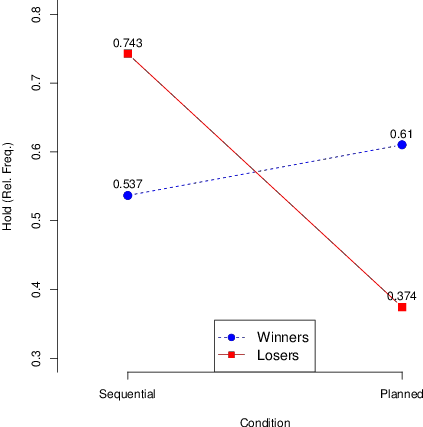
Figure 1 provides a representation of the relative frequency of hold choices in the two choice protocols (Sequential/Planned), for winners and losers in Phase 1 of the High Endowment condition.9
Figure 1 highlights a cross-over interaction effect between experiencing a win or a loss and the choice protocol adopted to collect investment choices. In Sequential, the frequency of hold is higher among losers than among winners (0.743 vs. 0.537, respectively), with the difference in hold rates being statistically significant according to non-parametric tests (Wilcoxon signed rank test, p=0.002).10 In contrast, in Planned losers are less likely to hold on to the investment than winners (0.374 vs. 0.610, respectively) (Wilcoxon signed rank test, p-value<0.001). Figure 1 also illustrates that the shift across choice conditions is mainly due to losers’ choices. Non-parametric tests confirm that only choices of losers significantly differ across the two conditions while those of winners do not (Wilcoxon Rank sum test, p-value<0.001 and p-value=0.268, respectively).11
Table 3 reports a description of hold rates in the robustness check conditions. The left panel reports about outcomes in Phase 2 of the High Endowment condition. The right panel reports about the choices in the Low Endowment condition, for which only the Sequential protocol is implemented.
Table 3: Hold rates of winners/losers across conditions.
Phase 2
SequentialSequential Planned Phase 1 Phase 2 Winners 0.583 0.559 0.532 0.550 Losers 0.607 0.477 0.676 0.600
In Phase 2 of the High Endowment condition (left panel of Table 3), no significant differences are observed when comparing winners and losers in Sequential and Planned (Wilcoxon Signed Rank test, p=0.883 and p=0.149, respectively). In the Low Endowment condition (right panel of Table 3), a marginally significant difference is registered when comparing hold rates of winners and losers in Phase 1, but not in Phase 2 (Wilcoxon Signed Rank test, p=0.099 and p=0.883, respectively).
The robustness check shows that the disposition effect highlighted by Figure 1 is observed, though to a lower extent, also when starting with a smaller endowment that affects the framing of losses. Furthermore, choices in Phase 2 show that the effects of Phase 1 are essentially linked to actually experiencing a loss/win and not to different levels of wealth of winners and losers after the first investment realization.12
The evidence collected here provides strong support for the existence of the disposition effect, when choices are taken sequentially. The asymmetry in liquidation patterns is mainly driven by a sustained propensity to hold on to the investment among losers. However, when choices are planned, a reverse disposition effect is observed, with losers less likely to hold on to their investment than in the sequential condition in which no reaction to losses must be planned. While the behavior of winners does not significantly differ across the two choice protocols, the behavior of losers changes substantially, thus reversing the disposition effect. Given that the same stochastic process is implemented in the two elicitation methods (i.e., the roll of a die), differences observed suggest that the disposition effect is more likely due to asymmetries in preferences between losers and winners than to biased beliefs.
The study presents some novel evidence about the role of investment planning in the disposition effect reversal. In related work, Weber and Zuchel (2005) identify the disposition effect when choices are taken in a context that promotes the perception of a strong connection between sequential choices (Portfolio), but identify a (weak) reversed disposition effect when choices are more likely to be perceived as segregated (Lottery). The authors argue that in the Portfolio setting the first risky choice in a sequence is more likely to be perceived as initiating a course of actions. This perception, in turn, may trigger an emotionally-laden escalation of commitment aimed at reverting a former loss by undertaking more risk in future choices. From this perspective, our Sequential condition is likely to create a closer connection between choices than the Planned condition, as in the former condition the second choice is taken just after experiencing the outcome of the first choice. Thus, it may be that the Sequential condition fosters escalation of commitment and the associated disposition effect.
Another important difference between the two choice protocols is that in Sequential the investors are aware of the actual outcome of their investment before choosing whether to hold on to it or not. Differently, in Planned the investors do not experience the joy/disappointment of a good/bad investment but are only asked to anticipate it. This may have important implications for investor’s self-image, a key element of the disposition effect (Shefrin & Statman, 1985) and of realization utility (Barberis & Xiong, 2009; Imas, 2016). Given that the differences between the two elicitation mechanisms are mainly due the behavior of losers, it may be that the impulse to not realize a loss and preserve one’s self-image is much stronger when the loss is actually experienced than when it is only anticipated. Further research is needed on this, in particular on why the Planned condition not only hampers the disposition effect but, actually, leads to its reversal.
The results presented here are in line with those of Imas (2016), who reports that more risk is borne after a paper loss than before it. Like Imas (2016), I also document a preference reversal in dynamic decisions. However, I focus on the relevance of incentive-compatible planning in a context of paper losses. I show that the definition of binding trading strategies reverses the disposition effect. This finding complements evidence collected by Fischbacher et al. (forthcoming), showing that the adoption of stop-loss/take-gain rules has consequences for the disposition effect. The authors also report evidence of a reversal in the disposition effect when the trading rules are available, though the effect seems more moderate than what documented here.
Interestingly, Fischbacher et al. (forthcoming) notice that their gain-take/stop loss rules work asymmetrically and provide a self-control device only for losers who are reluctant to sell, but not for winners who are too eager to sell. The Planned condition presented here overcomes this problem by providing winners with an effective commitment device.13 However, the results show that the behavior of winners is not significantly affected by the existence of such a commitment device and the reversal in the disposition effect is driven by losers.
My results, together with evidence emerging from the related studies reviewed above, may inform the design of efficient automatic stopping rules in investment choices. The definition of binding investment strategies, focused on the automatic realization of losses, may help curb the negative consequences of the disposition effect for portfolio management.
Barberis, N., & Xiong, W. (2009). What drives the disposition effect? an analysis of a long-standing preference-based explanation. The Journal of Finance, 64(2), 751–784.
Brandts, J., & Charness, G. (2000). Hot vs. cold: Sequential responses and preference stability in experimental games. Experimental Economics, 2(3), 227–238.
Chen, G., Kim, K. A., Nofsinger, J. R., & Rui, O. M. (2007). Trading performance, disposition effect, overconfidence, representativeness bias, and experience of emerging market investors. Journal of Behavioral Decision Making, 20(4), 425–451.
Coval, J. D., & Shumway, T. (2005). Do behavioral biases affect prices? The Journal of Finance, 60(1), 1–34.
Camerer, C., & Ho, T.-H. (1994). Violations of the betweenness axiom and nonlinearity in probability. Journal of Risk and Uncertainty, 8(2), 167–196.
Fischbacher, U. (2007). z-Tree: Zurich Toolbox for Ready-made Economic Experiments. Experimental Economics, 10(2), 171–178.
Fischbacher, U., Hoffmann, G., & Schudy, S. (forthcoming). The causal effect of stop-loss and take-gain orders on the disposition effect. Review of Finance, x(x), xx–xx.
Frazzini, A. (2006). The disposition effect and underreaction to news. The Journal of Finance, 61(4), 2017–2046.
Frydman, C., Barberis, N., Camerer, C., Bossaerts, P., & Rangel, A. (2014). Using neural data to test a theory of investor behavior: An application to realization utility. The Journal of Finance, 69(2), 907–946.
Frydman, C., & Rangel, A. (2014). Debiasing the disposition effect by reducing the saliency of information about a stock’s purchase price. Journal of Economic Behavior & Organization, 107, 541–552.
Genesove, D., & Mayer, C. (2001). Loss aversion and seller behavior: Evidence from the housing market. The Quarterly Journal of Economics, 116(4), 1233–1260.
Grinblatt, M., & Han, B. (2005). Prospect theory, mental accounting, and momentum. Journal of Financial Economics, 78(2), 311–339.
Heath, C., Huddart, S., & Lang, M. (1999). Psychological factors and stock option exercise. The Quarterly Journal of Economics, 114(2), 601–627.
Imas, A. (2016). The realization effect: Risk-taking after realized versus paper losses. American Economic Review, 106(8), 2086–2109.
Kahneman, D., & Tversky, A. (1979). Prospect Theory: An Analysis of Decision under Risk. Econometrica, 47(2), 263–291.
Kaustia, M. (2010). Prospect theory and the disposition effect. Journal of Financial and Quantitative Analysis, 45(3), 791–812.
Langer, T., & Weber, M. (2008). Does commitment or feedback influence myopic loss aversion? An experimental analysis. Journal of Economic Behavior & Organization, 67(3), 810–819.
Odean, T. (1998). Are investors reluctant to realize their losses? The Journal of Finance, 53(5), 1775–1798.
Prelec, D. (1998). The probability weighting function. Econometrica, 66(3), 497–527.
Shefrin, H., & Statman, M. (1985). The disposition to sell winners too early and ride losers too long: Theory and evidence. The Journal of Finance, 40(3), 777–790.
Shiv, B., Loewenstein, G., Bechara, A., Damasio, H., & Damasio, A. R. (2005). Investment behavior and the negative side of emotion. Psychological Science, 16(6), 435–439.
Thaler, R. H. (1999). Mental accounting matters. Journal of Behavioral Decision Making, 12(3), 183–206.
Tversky, A., & Kahneman, D. (1986). Rational choice and the framing of decisions. The Journal of Business, 59(4), S251–S278.
Tversky, A., & Kahneman, D. (1992). Advances in prospect theory: Cumulative representation of uncertainty. Journal of Risk and Uncertainty, 5(4), 297–323.
van Rooij, M., Lusardi, A., & Alessie, R. (2011). Financial literacy and stock market participation. Journal of Financial Economics, 101(2), 449 – 472.
Weber, M., & Camerer, C. F. (1998). The disposition effect in securities trading: an experimental analysis. Journal of Economic Behavior & Organization, 33, 167–184.
Weber, M., & Zuchel, H. (2005). How do prior outcomes affect risk attitude? comparing escalation of commitment and the house-money effect. Decision Analysis, 2(1), 30–43.
Wu, G., & Gonzalez, R. (1996). Curvature of the probability weighting function. Management Science, 42(12), 1676–1690.
Cumulative Prospect Theory provides us with a guidance to obtain some testable predictions in the experiment (for previous applications, see also Weber and Camerer, 1998, and Imas, 2016). For simple two-outcome prospects like those considered here, the value of a prospect is given by V(x1, x2; p1, p2)=w(p2)v(x2)+[1−w(p2)]v(x1), where x2 and x1 are the outcomes of the risky prospects, measured as deviations from a reference point, with the highest outcome in absolute value being x2, and p1 and p2 being the probabilities of the two outcomes. The weighting function w(p) maps probabilities into decision weights and Tversky and Kahneman (1992) suggest the following functional form for w(p): w(p)=pγ/[pγ+(1−p)γ](1/γ) (for an alternative specification, see Prelec, 1998). Concerning the value function v(x), Tversky and Kahneman propose the following: v(x)=xα for gains (x>0) and v(x)=−λ(−xα) for losses (x<0). The parameter λ captures loss aversions and here I adopt the value estimated by Tversky and Kahneman, λ=2.25. The parameter α > 0 captures the curvature of the value function and for α<1 those experiencing a gain relative to a reference point are risk-averse while those experiencing a loss are risk-seeking (reflection effect).
To derive a testable prediction, I assume that subjects who obtain a loss in the first roll of the die “move” to the loss domain and subjects who obtain a win “move” to the gain domain. When that is the case, the choice to hold or sell the investment is different for a winner and a loser. As an example, for the fair Prospect #3 a loser faces a choice between a sure loss of 40 when selling and a gamble giving a loss of 2× 40 with probability p=0.5 and no loss with p=0.5 when holding. For any level of risk-seekingness, the uncertain loss of 40 in expected value is always preferred to the sure loss of 40. In contrast, a winner will always choose to sell the fair prospect rather than hold on to it because of risk aversion.14
Table A1 provides a representations of the α restrictions required to observe a sell after a win and a hold after a loss, i.e., the disposition effect.
Prospect sell|win hold|loss
As Table A1 shows, for α ≤ 0.52 the disposition effect is observed in all prospects, but Prospect #1.15 In the latter, the investors should sell their investment after a loss, for any admissible value of α.
Table A2 displays the relative frequency of subjects who choose to hold on to their investments after the first die roll, conditional upon choice protocol (Sequential/Planned), phase (Phase1/Phase 2), prospect (#1 … #5), and outcome of the first roll of the die (Winners/Losers).
Table A2: Hold rates of winners/losers across conditions.
Phase 1 Phase 2 Prospect Losers Winners Diff Losers Winners Diff Sequential High Endowment #1 (+20/-40) 0.500 0.250 +0.250 0.300 0.333 -0.033 #2 (+30/-40) 0.640 0.429 +0.211 0.467 0.450 +0.017 #3 (+40/-40) 0.706 0.538 +0.168 0.633 0.633 0.000 #4 (+50/-40) 0.955 0.632 +0.323 0.817 0.667 +0.150 #5 (+60/-40) 0.963 0.818 +0.145 0.817 0.833 -0.016 Low Endowment #1 (+20/-40) 0.588 0.423 +0.165 0.367 0.383 -0.016 #2 (+20/-40) 0.640 0.486 +0.154 0.517 0.450 +0.067 #3 (+40/-40) 0.654 0.588 +0.066 0.600 0.483 +0.117 #4 (+50/-40) 0.667 0.515 +0.152 0.750 0.733 +0.017 #5 (+60/-40) 0.833 0.633 +0.200 0.767 0.700 +0.067 Planned High Endowment #1 (+20/-40) 0.256 0.462 -0.206 0.231 0.308 -0.077 #2 (+30/-40) 0.385 0.615 -0.230 0.410 0.385 +0.025 #3 (+40/-40) 0.282 0.641 -0.359 0.538 0.538 +0.000 #4 (+50/-40) 0.462 0.667 -0.205 0.564 0.769 -0.205 #5 (+60/-40) 0.487 0.667 -0.180 0.641 0.795 -0.154
The upper panel of Table A2 illustrates hold rates in the Sequential condition. In Phase 1 the percentage of losers holding on to their investment is always larger than the percentage of winners, both in the High and in the Low Endowment condition. In contrast, the hold rates in Phase 2 are similar among losers and winners and the pattern of hold rates is more faceted.
The lower panel illustrates hold rates in the Planned condition. In Phase 1 hold rates are always higher among winners than among losers, in contrast to what observed in the Sequential condition. Differences in hold rates between winners and losers are smaller in Phase 2 than in Phase 1.
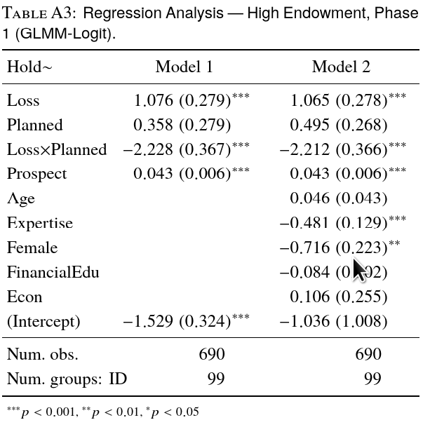
Table A3 reports a regression analysis about the determinants of the decision to hold on to the investment.16 The dependent variable Hold captures the decision to hold (Hold=1) or sell (Hold=0) the investment. The Loss variable is equal to 1 when the subject suffered a loss in the first roll of the die, and equal to 0 otherwise. Planned is a dummy variable equal to 1 when choices are collected via the Planned choice protocol and equal to 0 when choices are collected via the Sequential protocol. Prospect captures the size of the winning outcome and measures the expected value of each prospect (the losing outcome is always equal to -40).
In Model 2, I also check for self-reported expertise in finance (Expertise), gender (Female), performance in the administered financial education questionnaire (FinancialEdu), whether their study major is economics/business administration or not (Econ) and age (Age).
The regression analysis confirms that those experiencing a loss are more likely to hold on to the investment than those experiencing a win, when choices are taken in the Sequential condition. However, a non-removable interaction between the loss and the Planned condition is observed. A Linear hypothesis test confirms that in the Planned condition the situation reverses and the losers are less likely to hold on to the investment than the winners (Chi-squared test, p-value<0.001). The regression also shows that subjects correctly react to incentives and are more likely to hold on to the investment for prospects with higher expected value. These findings are robust when controlling for a few socio-demographic variables, as shown by Model 2. Furthermore, Model 2 suggests that females and subjects that are more competent in financial issues are less likely to hold on to the investment.
Note: the label [Common] identifies instructions which are common to Sequential and Planned choice protocols; the label [HighEndow.Seq] identifies instructions which refer exclusively to the High Endowment/Sequential condition; the label [LowEndow.Seq] identifies instructions which refer exclusively to the Low Endowment/Sequential condition and the label [Planned] identifies instructions which refer exclusively to the Planned choice protocol.
[Common] You earned €2.50 for showing up in time. We kindly ask you to read the instructions carefully and in silence. You must not talk to any other subject in the experiment. If you have any doubts, please raise your hand. A staff member will answer your question, privately. Any conduct interfering with the regular working of the experiment will be asked to leave the room and no payment will be made.
[Common] The experiment is made up of two independent parts. You will be given instructions for the second part only at the end of the first part.
[Common] The experiment allows you to earn an amount in Euro. In the course of the experiment, you will use experimental currency units (ECU) instead of Euro. At the end of the experiment, 20 ECU will be exchanged for €1 and the amount in Euro will be paid out in cash (For example, earnings of 100 ECU will be exchanged at the end of the experiment for €5).
[Common] Your final earnings in the experiment amount to the sum of earnings in the first and in the second part.
[LowEndow.Seq] At the end of the experiment you may register negative earnings. Any negative amount earned will be deducted from the show-up fee you have already earned for showing up on time. For example, if you earn €-1 you will receive only €1.50 for showing up on time. The €2.50 earned for showing up on time is always enough to cover potential negative earnings in the experiment and you will never be asked for money to compensate for negative earnings.
Note: in the original instructions the letter E is replaced by 60 in the Low Endowment/Sequential condition and by 100 in the other conditions. 10pt
[Common] This part is made up of 5 independent rounds. In each round, you are given E UMS. You must allocate the E UMS by choosing to invest in good X or good Y. Both goods have a price of E UMS. One of the two goods will yield a gain, the other will yield a loss; the magnitude of losses and gains changes every round and you will be informed at the beginning of each round about these changes.
[Common] After you have invested in one of the two goods, a randomly picked subject tosses a die: when the outcome is a number equal to or lower than 3, good X is selected and yields a gain while good Y yields a loss; when the outcome is a number greater than 3, good Y is selected and yields a gain while good X yields a loss.
[HighEndow.Seq, LowEndow.Seq] After the initial draw, you can choose whether to keep or sell your good.
[Planned] At the beginning of each round, you can choose whether to keep or sell your good after the first toss of the die. The choice must be taken before the toss and, thus, without knowing the outcome. This means you must choose whether to keep or sell your good, both in the case of you obtaining a gain (scenario 1) and obtaining a loss (scenario 2) in the first toss of the die. The choice made in correspondence to the outcome of the first toss of the die is binding and cannot be changed.
[Common] If you choose to sell the good, your earnings are given by the value of the good after the first draw. If you choose to keep the good, your earnings are conditional upon the toss of a die performed by a subject picked at random: when the outcome is a number equal to or lower than 3 (1, 2, or 3), good X is selected and yields a gain, while good Y yields a loss; when the outcome is a number greater than 3 (4, 5, or 6), good Y is selected and yields a gain, while good X yields a loss. The magnitude of losses and gains changes every round and you will be told at the beginning of each round about these changes.
[Common] At the end of the experiment, only one of the five rounds that belong to the first part is randomly selected for payment. You will be told the chosen round at the end of second part.
[Common] This part is made up of 10 independent rounds. In each round, you are given an endowment in UMS. The endowment changes every round and you will be told at the beginning of each round about these changes. You must allocate the UMS by choosing to invest in good X or good Y. Both goods have a price equal to your UMS endowment in that round.
[Common] After you have invested in one of the two goods, you can choose whether to keep or sell your good. If you choose to sell the good, your earnings are given by the value of the good after the first draw. If you choose to keep the good, your earnings are conditional upon the toss of a die performed by a subject picked at random: when the outcome is a number equal to or lower than 3 (1, 2, or 3), good X is selected and yields a gain, while good Y yields a loss; when the outcome is a number greater than 3 (4, 5, or 6), good Y is selected and yields a gain, while good X yields a loss. The magnitude of losses and gains changes every round and you will be told at the beginning of each round about these changes.
[Common] At the end of the experiment, only one of the five rounds that belong to the second part is randomly selected for payment.
Francesco Nadalini is acknowledged for his assistance in an early stage of this work. Dominique Cappelletti helped me with her constant support. The editor and the anonymous referees provided a useful and competent guidance in the revision of the manuscript. Participants in seminars and conferences are acknowledged for their comments and suggestions. The usual caveat applies.
Copyright: © 2017. The authors license this article under the terms of the Creative Commons Attribution 3.0 License.
This document was translated from LATEX by HEVEA.