Judgment and Decision Making, Vol. 11, No. 4, July 2016, pp. 361-379

People often make more rational choices between monetary prospects when their choices will be played out many times rather than just once. For example, previous research has shown that the certainty effect and the possibility effect (two common-ratio effects that violate expected utility theory) are eliminated in multiple-play decisions. This finding is challenged by seven new studies (N = 2391) and two small meta-analyses. Results indicate that, on average, certainty and possibility effects are reduced but not eliminated in multiple-play decisions. Moreover, in our within-participants studies, the certainty and possibility choice patterns almost always remained the modal or majority patterns. Our primary results were not reliably affected by prompts that encouraged a long-run perspective, by participants’ insight into long-run payoffs, or by participants’ numeracy. The persistence of common-ratio effects suggests that the oft-cited benefits of multiple plays for the rationality of decision makers’ choices may be smaller than previously realized.

Keywords: common-ratio effect, reverse common-ratio effect, certainty effect, possibility effect, multiple play, repeated play.

1  Introduction

In many instances, people make better, more rational decisions when they take a broad view of their situation rather than a narrow view (Kahneman & Lovallo, 1993; Read, Loewenstein & Rabin, 1999). For example, buying an extended warranty for a particular electronic device may seem appealing when one is thinking only about that device, but thinking more broadly may make it easier to realize that the aggregate cost of such warranties over many appliances and devices almost certainly exceeds the expected cost of possible failures. Assuming that such insurance is a moneymaker for the seller, insuring against relatively small losses that one can afford doesn’t make much sense, at least in terms of expected value (EV). Although this argument can be — and perhaps should be — applied to an individual purchase, many people find the notion of an expectation to be more compelling when they consider aggregating over numerous purchases.

Indeed, an ever-growing body of research has indicated that people are more likely to make decisions that are in accord with EV theory or expected utility (EU) theory when they consider risky options whose outcomes will be aggregated over many plays (for a review, see Wedell, 2011). For example, people are more likely to accept mixed gambles (those involving the possibility of a gain or a loss) with positive EVs when they will be played multiple times rather than just once (Benartzi & Thaler, 1999; DeKay & Kim, 2005; Klos, 2013; Klos, Weber & Weber, 2005; Langer & Weber, 2001; Montgomery & Adelbratt, 1982; Redelmeier & Tversky, 1992; Wedell & Böckenholt, 1994). Similarly, for gambles involving either gains or losses (but not both), people are more likely to choose the higher-EV option in multiple play than in single play (Camilleri & Newell, 2013; Haisley, Mostafa & Loewenstein, 2008; Joag, Mowen & Gentry, 1990; Li, 2003; Su et al., 2013; but see Chen & Corter, 2006, for conflicting results). For gains, Wulff, Hills, and Hertwig (2015) recently extended this result to the situation in which participants learn about the probabilities and outcomes of the gambles via sampling (i.e., decisions from experience rather than decisions from description; for reviews, see Hertwig, 2015; Hertwig & Erev, 2009). Additional studies have indicated that preference reversals (Wedell & Böckenholt, 1990), ambiguity aversion (Liu & Colman, 2009), and the description-experience gap (Camilleri & Newell, 2013) are also reduced in multiple play. Although most of these studies have involved monetary gambles, the results appear to extend to other situations as well (DeKay & Kim, 2005; Liu & Colman, 2009; Joag et al., 1990), at least when participants consider the aggregation of outcomes over multiple plays to be reasonable (DeKay & Kim, 2005; for related results, see DeKay, 2011; DeKay, Hershey, Spranca, Ubel & Asch, 2006).¹

1.1  Common-ratio effects

Previous research has also indicated that common-ratio effects are eliminated in multiple-play decisions (Barron & Erev, 2003, Study 5; Keren, 1991; Keren & Wagenaar, 1987). These effects, and their moderation in multiple play, are the focus of this article. Demonstrations of common-ratio effects require two choice problems: a scaled-up problem and a scaled-down problem. The possible outcomes in the two problems are identical, but the probabilities of the nonzero outcomes in the scaled-down problem are decreased by the same factor relative to corresponding probabilities in the scaled-up problem. For example, in one version that we use, the scaled-up problem is a choice between Option A (a 100% chance of $60) and Option B (an 80% chance of $100, otherwise $0; hereafter, we omit the $0 outcome). In the scaled-down problem, the probabilities of winning in both options are divided by four (the common ratio) to yield a choice between A^′ (a 25% chance of $60) and B^′ (a 20% chance of $100). The percentage of participants choosing the higher-EV option (B or B^′, depending on the problem) is typically much higher in the scaled-down problem than in the scaled-up problem; this discrepancy is the common-ratio effect. In this particular example, the discrepancy is also called a certainty effect (Kahneman & Tversky, 1979; Keren & Wagenaar, 1987), because one of the options in the scaled-up problem is a sure thing.

A common-ratio effect that involves very low probabilities in the scaled-down problem is called a possibility effect (Keren & Wagenaar, 1987). In our version, the scaled-up problem is a choice between C (a 90% chance of $50) and D (a 45% chance of $120) and the scaled-down problem is a choice between C^′ (a 2% chance of $50) and D^′ (a 1% chance of $120), where the chances of winning have been divided by 45. As before, the higher-EV option (D or D^′) is typically much more popular in the scaled-down problem.

The modal choice pattern in these problems (e.g., choosing C in the scaled-up version and D^′ in the scaled-down version of the possibility-effect example) violates EU theory. Under EU theory, choosing C over D implies that .90 × u($50) > .45 × u($120), which simplifies to u($50)/u($120) > 0.5. Similarly, choosing D^′ over C^′ implies that .02 × u($50) < .01 × u($120), which simplifies to u($50)/u($120) < 0.5. These conclusions are contradictory; there is no utility function consistent with both preferences. By the same logic, the opposite patterns (choosing B and A^′ in the certainty-effect example or D and C^′ in the possibility-effect example) also violate EU theory. These reverse patterns are less well known, but are common for some sets of problems (e.g., when the probabilities in the scaled-up and scaled-down problems differ by a smaller factor; Blavatskyy, 2010; Nebaut & Dubois, 2014).²

When discussing these issues, we find it useful to distinguish between an effect and a choice pattern. For the problems considered in this article, we define the common-ratio effect (and the two special cases, the certainty effect and the possibility effect) as the empirical observation that participants are more likely to choose the riskier, higher-EV option in the scaled-down problem than in the corresponding scaled-up problem. This definition applies equally to between-participants and within-participants designs and is independent of theoretical explanations (e.g., regarding the relative weighting of certain and uncertain outcomes; Kahneman & Tversky, 1979).³ Later in this article, we discuss how the certainty effect, for example, reflects the relative frequencies of participants with the certainty choice pattern (A and B^′ in the above example) and participants with the reverse certainty choice pattern (B and A^′). Although these patterns are discernable only in within-participants designs in which participants respond to both the scaled-up and scaled-down problems, they are assumed to be present but unmeasured in between-participants designs (without this assumption, it would be impossible to infer utility violations from between-participants data).

In previous research, Keren and Wagenaar (1987, Study 1 and follow-up) showed that the certainty effect (or more precisely, a near-certainty effect, as they used a probability of .99 rather than 1.00 in their scaled-up problem) was eliminated when the gambles would be played ten times rather than just once. They obtained this result for both gains and losses in their Study 1. In their Study 2, Keren and Wagenaar showed that the possibility effect was eliminated when the gambles would be played 100 times instead of once. Keren (1991) replicated Keren and Wagenaar’s results for the certainty effect using two different sets of problems and only five plays in the multiple-play condition. In all of these studies, the common-ratio effects disappeared because the frequency of choosing the higher-EV option in the scaled-up problem increased in multiple play, whereas the frequency of choosing the higher-EV option in the scaled-down problem stayed about the same or increased only slightly. Li (2003) also reported that the frequency of choosing the higher-EV option in a scaled-up certainty-effect problem increased in multiple play, but that study did not include a corresponding scaled-down problem. Finally, Barron and Erev (2003, Study 5) reported that the certainty effect was eliminated and nearly reversed when very small gambles would be played 100 times.⁴ However, in contrast to the other studies (and the effect of multiple plays more generally), this result was due primarily to a large decrease in the frequency of choosing the higher-EV option in the scaled-down problem. Taken together, these studies provide strong evidence that common-ratio effects are reduced or eliminated in multiple play, though Barron and Erev’s results differ from the others in important ways. Table S.1 in the Supplement lists the gambles used in these studies.

1.2  Theoretical explanations

There is no generally accepted explanation for why people exhibit common-ratio effects in single-play choices. Explanations as varied as prospect theory (Kahneman & Tversky, 1979; Tversky & Kahneman, 1992), the transfer of attention exchange model (Birnbaum, 2008), the priority heuristic (Brandstätter, Gigerenzer & Hertwig, 2006), Mukherjee’s (2010) dual-system model, decision field theory with distraction (Bhatia, 2014), and EU models with noise or sequential sampling (Loomes, 2015) can account for at least some common-ratio effects. However, even theories that can explain common-ratio effects may fail to do so in specific instances. For example, Tversky and Kahneman’s (1992) best-fitting parameter values for cumulative prospect theory do not predict the possibility effect in Kahneman and Tversky’s (1979) original example.⁵ A more serious challenge is that none of these theories tested thus far can explain the reverse common-ratio effects that occur for other pairs of problems (Blavatskyy, 2010; Nebaut & Dubois, 2014).

Regarding the general effects of multiple plays, Wedell (2011) noted that there are two basic types of explanations: those that assume a common process in single and multiple play and those that do not. In one example of a common-process explanation, Langer and Weber (2001) demonstrated that cumulative prospect theory can account for participants’ choices regarding mixed, positive-EV gambles in both single and multiple play when participants are shown (and the theory is applied to) the aggregate distribution of possible outcomes in the multiple-play condition. This result is consistent with the fact that participants are especially likely to accept multiple plays of (most) such gambles when presented with the full distribution of possible outcomes (Benartzi & Thaler, 1999; DeKay, 2011; DeKay & Kim, 2005; Klos, 2013; Langer & Weber, 2001; Redelmeier & Tversky, 1992; for an exception, see Keren, 1991). The generality of common-process explanations is limited, however, by the difficulty of envisioning or calculating the relevant features of outcome distributions when they are not provided (Benartzi & Thaler, 1999; Klos, 2013; Klos et al., 2005). This problem may be especially acute for common-ratio effects because most of the choices involve two risky options rather than one.

In our view, a more likely explanation for the effects of multiple plays is that the decision processes are more thorough and integrative in multiple play than in single play (Wedell, 2011). For example, participants find EV information to be more relevant (Montgomery & Adelbratt, 1982) and report using more complex strategies (Wedell & Böckenholt, 1994) in multiple-play decisions. Evidence from functional measurement (Joag et al., 1990) and eye tracking (Su et al., 2013) also indicates that participants are more likely to use multiplicative or weighting-and-adding processes in multiple play than in single play. Most recently, Wulff et al. (2015) reported that in a decisions-from-experience task involving pairs of gambles, participants who anticipated making a multiple-play choice rather than a single-play choice tried out the gambles more times before deciding which one to play. Perhaps ironically, these studies suggest that people are more likely to use complicated decision strategies in multiple play, where such strategies are more difficult to apply.

1.3  Seven new studies

In what follows, we report seven new studies regarding the possible reduction or elimination of common-ratio effects in multiple-play decisions. Our goal was not to resolve the process issues raised above, though some of our data do bear on the question of whether proper aggregation of long-run payoffs is sufficient to eliminate common-ratio effects. Nor was our goal to replicate or not replicate other researchers’ results, though that is how the project evolved. Instead, our original intent was to assess whether the elimination of common-ratio effects in multiple-play decisions — a finding that we considered relatively well established — would be moderated by participants’ views regarding the reasonableness of aggregating outcomes over multiple plays (i.e., the perceived fungibility of the outcomes; DeKay & Kim, 2005; see the Supplement for details regarding our rationale). Although we predicted that multiple plays would diminish the certainty and possibility effects when outcome aggregation is reasonable, both effects remained large and significant in multiple-play decisions involving monetary gambles for oneself. Surprised by these initial results, we conducted several additional studies in which we attempted to strengthen the multiple-play manipulation by (a) increasing the number of plays, (b) improving the clarity and salience of the relevant wording, (c) creating additional conditions that were intended to encourage participants to think about aggregate outcomes in multiple play, and (d) playing participants’ choices for real money (in one study). Despite these and other efforts (e.g., using both within- and between-participants designs), certainty and possibility effects almost always remained significant in multiple-play decisions.

For ease of exposition, we present our seven studies together rather than separately. We first describe our general experimental approach, noting the most important differences among our studies, and then use simple graphs to compare our results to those of earlier authors. After illustrating our basic statistical model using data from a few example studies, we present two small meta-analyses (separate analyses for certainty and possibility effects) that integrate the results of our new studies with those from previous research. We then look in greater detail at the choice patterns in our within-participants studies. Finally, we examine the additional conditions that were designed to encourage participants to think about aggregate outcomes and we assess whether the effects of multiple plays are moderated by two individual differences. Considering the old and new studies together, the overall results indicate that common-ratio effects are much more persistent in multiple play than previously thought.

2  Method

Table 1 provides an overview of study characteristics, sample sizes, and participant demographics in our seven studies.

2.1  General procedures

In each study, we randomly assigned participants to the 1-play, 10-play, and 100-play conditions. The first part of Study 1 omitted the 100-play condition, whereas Studies 4–7 omitted the 10-play condition (i.e., we increased the number of plays in the later studies). In our standard design, participants in each condition made 11 choices between options like those described in Table 2, with each problem shown on a separate screen of the computer-based survey. For example, Problem 10 was presented as follows in the single-play [multiple-play] condition:

Option A:

45% chance [on each gamble] that you get $120

55% chance [on each gamble] that you get no money

Option B:

90% chance [on each gamble] that you get $50

10% chance [on each gamble] that you get no money⁶

---

Table 1: Study characteristics, sample sizes, and participant demographics

Study	Location and participant recruitment	Administration and compensation	Manipulation of choice problems	Multiple plays	Payoff multiplier for multiple plays
1	Carnegie Mellon electronic	Online; $10	Within (and between)	10 and 100b	1
	bboards, email lists, and fliers		participantsa
2	Carnegie Mellon campus sidewalk	On the sidewalk; candy bar	Between participants	10 and 100	1
3	Ohio State psychology	In lab; course credit	Within participants	10 and 100	1
	participant pool
4	Ohio State psychology	In lab; course credit	Within participants	100	1 and 0.01 (cents)
	participant pool
5	Ohio State psychology	In lab; course credit plus	Within participants	100	0.01 (cents)
	participant pool	cash outcome of one option
6	Ohio State psychology	In lab; course credit	Within participants	100	1
	participant pool
7	Amazon Mechanical Turk, US only	Online; $0.50	Within (and between) participantsa	100	1

	Study		Participants excluded		Final N		Student status		Female	Mean age (range)
	1		9c		201		48% UG, 30% GS, 22% NS		50%	24 (18–58)
	2		1d		490		87% UG, 6% GS, 7% NS		44%	24 (14–78)
	3		27c		343 (165 in SC)		UG		45%	20 (18–54)
	4		43c		373 (144 in SC)		UG		53%	19 (18–39)
	5		14c + 1e		184 (91 in SC)		UG		48%	20 (18–46)
	6		19c + 73f		101		UG		62%	19 (18–26)
	7		7d + 96f		699		—g		43%	34 (18–75)
Note. UG = undergraduates. GS = graduate students. NS = nonstudents. SC = standard conditions, with no additional questions or statements designed to encourage the long-run perspective.
a Because problem order was reversed for half of the participants, the first half of the data can be treated as a between-participants study.
b Study 1 had two parts: Study 1a involved 1 or 10 plays, whereas Study 1b involved 1, 10, or 100 plays. Otherwise, the questions were identical. See the Supplement for details.
c Excluded for failing the attention check and/or not answering a key choice question.
d Excluded for not answering a key choice question (there was no attention check).
e Excluded for suspecting that cash payments would not be made (they were).
f Excluded for failing the manipulation check.
g Not assessed.

---

Problems 2 and 8 (based on Keren, 1991) provided a within-participants test of the certainty effect (as in Kahneman & Tversky, 1979, and Barron & Erev, 2003) and Problems 4 and 10 (based on Keren & Wagenaar, 1987) provided a within-participants test of the possibility effect (as in Kahneman & Tversky, 1979). Treating problem as a within-participants variable allowed us to assess participants’ choice patterns, as noted above (in contrast, the number of plays was always a between-participants variable). Problem 6 provided an attention check in which one option dominated the other. Participants who did not chose the dominant option in Problem 6 or who did not make all four of the key choices (Problems 2, 4, 8, and 10) were excluded from all analyses. The six odd-numbered problems were included to reduce the likelihood that participants would notice the relationships between the problems of interest; these filler problems are not discussed further. In 5 of the 11 problems, the option presented first had the higher EV. Payoffs were hypothetical in all studies except Study 5 (see below).

---

Table 2: Critical problems, gambles, and expected values (EVs) in the single-play condition

	Higher-EV option			Lower-EV option
	Probability	Amount		Probability		Amount
Problem and label	of winning	to win	EV	of winning		to win	EV
2 (No certainty)	.20	$100	$20	.25		$60	$5
4 (Possible)	.01	$120	$1.20	.02		$50	$1
6 (Attention check)	.40	$80	$32	.30		$70	$21
8 (Certainty)	.80	$100	$80	1.00		$60	$60
10 (Probable)	.45	$120	$54	.90		$50	$45
Note. All options except the certain option in Problem 8 included a complementary outcome of “no money”. Labels and EVs were not shown to participants. The six odd-numbered problems were fillers and are omitted here. Studies 2 and 7 used only Problems 2, 4, 8, and 10. Gambles in Studies 4–6 had lower stakes (one tenth as large for these critical problems). Table S.2 in the Supplement lists all problems used in the single-play condition of Studies 1–7.

---

In the multiple-play conditions, participants were told that each of the two options “involves a series of ten [one hundred] monetary gambles.” After the options were described, but before participants made their choice, they were told, “Your choice between options A and B applies to all ten [one hundred] gambles.” Before the very first choice, participants were also told, “You may not choose option A for some gambles and option B for others.” In Experiments 4–7, they were also told, “Regardless of your choice, the outcome of any particular gamble in the sequence (say the 23rd gamble) has no effect on the outcome of any other gamble in the sequence (say the 24th gamble or the 67th gamble). Each gamble is independent of the others.” Study 7 included an additional analogy to “flipping a coin or rolling a die over and over again.”

For each problem, participants made a preference rating on a nine-point bipolar scale (omitted in Study 7) and then a binary choice. Beginning with Study 3, these questions stressed that the gamble would be played ONE, TEN, or ONE HUNDRED times. In this article, we focus almost exclusively on the binary choices, for consistency with previous research. In Study 7, we included the words ONE AND ONLY ONE play and ONE HUNDRED plays in the response options as well as the questions. In every study, participants answered a few debriefing questions and provided demographic information at the end of the survey.

2.2  Primary differences among studies

Study 1 had two parts. Study 1a was designed to assess the role of perceived fungibility in multiple-play decisions. In this article, we consider only those conditions involving monetary gambles for oneself (there were several other conditions; see the Supplement) and ignore all questions related to fungibility. In Study 1b, we simplified the design by using only monetary gambles for oneself, but added a 100-play condition to strengthen the multiple-play manipulation. The results of Studies 1a and 1b are combined for analysis.

The most obvious difference between our Study 1 and Keren and Wagenaar’s (1987) studies is that we assessed the certainty and possibility effects within participants (as did Barron & Erev, 2003, for the certainty effect) rather than between participants. In Study 2, we adopted a completely between-participants design similar to that in Keren and Wagenaar’s studies, with each participant making only one of the four key choices (Problem 2, 4, 8, or 10) in either the 1-play, 10-play, or 100-play condition. In order to collect a large sample relatively quickly, we administered the study as a short paper-based survey on a busy university sidewalk.

After Study 2, we returned to our within-participants approach. In addition to the standard conditions (described above), Studies 3–5 also included one or more conditions designed to encourage participants to adopt a long-run perspective. These conditions might be expected to facilitate the choice of the higher-EV option, thereby reducing the certainty and possibility effects, especially in multiple play. Additionally, because reasoning about gambles (and multiple plays of gambles) requires a degree of mathematical ability or intuition, we hypothesized that the effects of multiple plays might be more pronounced for participants who are better at math. In Studies 4–6, we examined the possible moderating effects of participants’ numeracy, defined as “the ability to process basic probability and numerical concepts” (Peters, Västfjäll, Slovic, Merz, Mazzocco & Dickert, 2006, p. 407; also see Peters, 2012), using an established eight-item scale (Weller, Dieckmann, Tusler, Mertz & Peters, 2013). We discuss these additional conditions and measures later, after our main results.

---

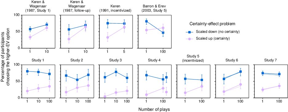
Figure 1: Percentages of participants choosing the higher-EV option in problems related to the certainty effect in previous studies (top) and in the standard conditions of our studies (bottom). In Study 4, the results for 100 plays with cents appear to the right of those for 100 plays with dollars. In Studies 6 and 7, solid lines show results for participants who answered the manipulation-check question correctly; dotted lines (without error bars) show results for all participants. Error bars indicate 95% CIs.

---

In Study 5, we used real monetary payoffs rather than hypothetical ones. To do so, we lowered the stakes in both the 1-play and 100-play conditions (see Table S.2 in the Supplement) and lowered the stakes in the 100-play condition even further, by using cents rather than dollars. We pretested these changes with hypothetical payoffs in Study 4, which had separate multiple-play conditions for dollars and cents. Reducing payments in proportion to the number of plays is a popular way to equate EVs and payoff ranges (but not risks) in the single- and multiple-play conditions (see, e.g., Keren & Wagenaar, 1987, Studies 1 and 2). Participants in our Study 5 played their chosen option in one of the 11 problems (selected at random) for real money before leaving the session. The gamble in the chosen option was played either one time (for dollars) or 100 times (for cents), depending on each participant’s condition.⁷

Although participants were reminded of the number of plays many times (e.g., the number ONE HUNDRED appeared 34 times in the standard multiple-play condition of Studies 4 and 5), the results made us wonder whether some participants had simply tuned out that information. Studies 6 and 7 included manipulation checks that asked participants how many times their chosen option would be played in each choice (Study 6) or in the choice they just made (Study 7). Our primary analyses are restricted to participants who answered correctly (including all participants yielded very similar results). Study 7 was our largest study, conducted on Amazon Mechanical Turk. It differed from the other studies in that participants answered either the two certainty-effect problems or the two possibility-effect problems, without any fillers. We had initially envisioned Study 7 as a much stronger version of our between-participants Study 2, but decided that there was no harm in adding a second problem. Because we manipulated problem order, the first half of the data could still be treated as a between-participants study (this was also true of Study 1, in which the order of the 11 problems was reversed for half of the participants). For additional details and the surveys themselves, see the Supplement.

---

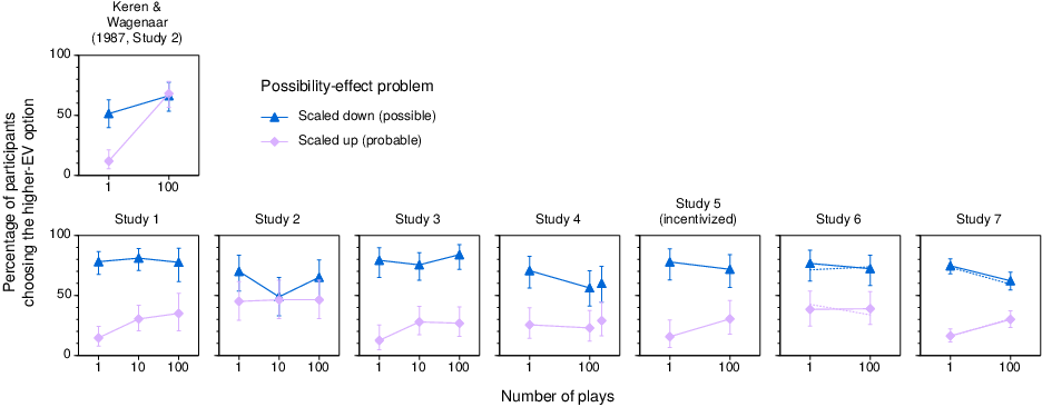
Figure 2: Percentages of participants choosing the higher-EV option in problems related to the possibility effect in a previous study (top) and in the standard conditions of our studies (bottom). In Study 4, the results for 100 plays with cents appear to the right of those for 100 plays with dollars. In Studies 6 and 7, solid lines show results for participants who answered the manipulation-check question correctly; dotted lines (without error bars) show results for all participants. Error bars indicate 95% CIs.

---

3  Results

3.1  Visual comparisons between studies

Figure 1 presents results for the certainty effect, with previous studies in the top row and the standard conditions of our studies in the bottom row. In each panel, a certainty effect occurred whenever the higher-EV option was significantly more likely to be chosen in the scaled-down problem, which did not include a certain option, than in the scaled-up problem, which did.

A few basic results are evident in the figure. First, certainty effects were obtained in the single-play conditions of all of the studies, though they were generally larger in our studies than in previous studies. Second, in the multiple-play conditions, certainty effects remained relatively large in most of our studies, whereas they essentially disappeared in Keren and Wagenaar’s (1987) and Keren’s (1991) studies and were reversed in Barron and Erev’s (2003) study (note the large drop for the scaled-down problem in Barron and Erev’s data). Certainty effects were somewhat smaller in multiple play than in single play in most of our studies as well, though the larger spread in our studies makes the magnitudes of these reductions difficult to assess visually. Finally, it appears that there was not a reliable difference between the results for 10 and 100 plays in our studies.

Figure 2 depicts remarkably similar results for the possibility effect. In each panel, a possibility effect occurred whenever the higher-EV option was significantly more likely to be chosen in the scaled-down problem than in the scaled-up problem. In most of our studies, possibility effects were large in both the single- and multiple-play conditions, in contrast to the disappearance of the effect in the multiple-play condition of Keren and Wagenaar’s (1987) study. Possibility effects were smaller in our between-participants Study 2 than in our other studies, but the results did not match those of Keren and Wagenaar’s study either. As was the case for certainty effects, there was no consistent difference between the results for 10 and 100 plays in our studies. Overall, certainty and possibility effects appeared more persistent in our studies than in previous studies.

In Studies 1–6, participants made a preference rating before choosing an option in each problem. Graphical results for mean preference ratings (see Figure S.1 in the Supplement) were nearly identical to those for choice proportions. Moreover, the choice-proportion results for Study 7, in which choices were not preceded by preference ratings, were very similar to those for Studies 1–6 (see Figures 1 and 2), suggesting that the preference ratings had little if any effect on participants’ subsequent choices. We do not consider the preference ratings further.

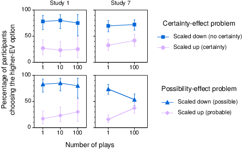
Because we manipulated problem order in Studies 1 and 7, considering only the first half of the data yielded a between-participants study in each case. Figure 3 indicates that the results for the first half of the data look similar to those for the full studies (see the corresponding panels in Figures 1 and 2). The one exception was that, in Study 7, the effect of multiple plays on the possibility effect was notably stronger when only the first half of the data was considered. However, in contrast to Keren and Wagenaar’s (1987, Study 2) results for the possibility effect (see Figure 2), about half of the reduction in Study 7 was due to a decrease in the percentage of participants choosing the higher-EV option in the scaled-down problem in multiple play (see Figure 3).

---

Figure 3: Percentages of participants choosing the higher-EV option in problems related to the certainty effect (top) and the possibility effect (bottom) in the first half of our Studies 1 and 7 (between-participants comparisons). Error bars indicate 95% CIs.

---

The apparent interactions in several panels of Figures 1–3 are nonremovable in the sense that they cannot be eliminated by a monotonic transformation of the measurement scale (Loftus, 1978; Wagenmakers, Krypotos, Criss & Iverson, 2013). The interactions in the older studies are nonremovable because they are crossover interactions: The lines either cross or touch (Loftus, 1978; Wagenmakers et al. used the term borderline nonremovable for cases in which the lines merely touch, because the equivalence is based on a statistical test). In most of our studies, the lines do not cross or touch in Figures 1–3. Nonetheless, the interactions are crossover interactions because the lines would cross or touch if the data were plotted differently, with problem on the horizontal axis and a separate line for each number of plays. Crossing would occur whenever the two lines in a panel of Figures 1–3 have opposite slopes, whereas touching would occur whenever one or both of the lines are essentially flat. The only obvious exception is for the certainty effect in Study 6 (see Figure 1), where both lines slope up. There is no apparent interaction in that panel and any interaction created as the result of a transformation would be removable. Nonremovability is important because it implies that the interactions are interpretable in terms of psychological processes (e.g., judgments of payoffs or risks) that are monotonically related to the dependent variable. It also means that the interactions reported in the following sections are not artifacts of the logistic transformation.

3.2  Illustrative analyses

For each effect (certainty or possibility) in each study, we used logistic regression to predict the choice of the higher-EV option on the basis of problem (scaled-up problem =
–1/2, scaled-down problem = +1/2), plays (single play =
–1/2, multiple play = +1/2), and their interaction. The variables were coded so that a positive effect of problem would indicate the expected certainty or possibility effect and a positive coefficient for plays would indicate a greater likelihood of choosing the higher-EV option in multiple play. A reduction in the magnitude of a certainty or possibility effect in multiple play would be evidenced by a negative coefficient for the interaction. For brevity, we present detailed results for only a few illustrative studies.

For Keren and Wagenaar’s (1987, Study 1) certainty-effect data (see Figure 1), there was a significant positive effect of problem, b = 0.71, 95% CI [0.39, 1.04], OR = 2.04, χ²(1) = 18.61, p < .001; a significant positive effect of plays, b = 0.88, CI [0.55, 1.20], OR = 2.40, χ²(1) = 28.38, p < .001; and a nearly significant negative interaction, b = –0.57, CI [–1.23, 0.08], OR = 0.56, χ²(1) = 2.93, p = .087. These statistics essentially recreate Keren and Wagenaar’s results, but with the addition of coefficients and confidence intervals. For Keren and Wagenaar’s (1987, Study 2) possibility-effect data (see Figure 2), all three effects were significant: b = 0.99, CI [0.45, 1.53], OR = 2.69, χ²(1) = 13.71, p < .001 for problem; b = 1.69, CI [1.15, 2.23], OR = 5.41, χ²(1) = 42.69, p < .001 for plays; and b = –2.14, CI [–3.22,
–1.06], OR = 0.12, χ²(1) = 16.02, p < .001 for the interaction. For both the certainty and possibility effects, the Problem × Plays interaction was attributable to the increased appeal of the higher-EV option in the scaled-up problem in multiple play.

In our Study 1, which had rather typical results for our studies, we used repeated-measures logistic regressions because each participant responded to both the scaled-up and scaled-down problems.⁸ For ease of comparison across studies, we ignored the distinction between the 10- and 100-play conditions in our primary models. For the certainty effect (see Figure 1), there was a significant positive effect of problem, b = 2.37, CI [1.85, 2.88], OR = 10.66, χ²(1) = 75.04, p < .001, but the effect of plays, b = 0.15, CI [–0.29, 0.60], OR = 1.17, χ²(1) = 0.46, p = .50, and the interaction, b = –0.78, CI [–1.81, 0.24], OR = 0.46, χ²(1) = 2.29, p = .13, were not significant. For the possibility effect in Study 1 (see Figure 2), there were significant positive effects of problem, b = 2.58, CI [2.02, 3.14], OR = 13.23, χ²(1) = 79.68, p < .001, and plays, b = 0.56, CI [0.12, 0.99], OR = 1.75, χ²(1) = 6.07, p = .013, but the interaction was not significant, b = –0.90, CI [–2.01, 0.21], OR = 0.41, χ²(1) = 2.60, p = .11.⁹ In contrast to Keren and Wagenaar’s (1987) results, the certainty and possibility effects remained significant in multiple play (see below). In summary, the results of our Study 1 did not replicate those of Keren and Wagenaar (1987) especially well, though the signs of the coefficients were the same in all of the above regressions.

---

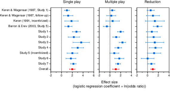
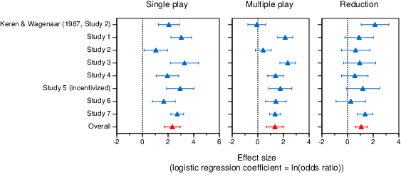
Figure 4: Meta-analysis results for the certainty effect in single- and multiple-play decisions. Error bars indicate 95% CIs.

---

---

Figure 5: Meta-analysis results for the possibility effect in single- and multiple-play decisions. Error bars indicate 95% CIs.

---

3.3  Two small meta-analyses

In order to resolve apparently conflicting results like those above, we conducted two small meta-analyses: one for the certainty effect (11 studies) and one for the possibility effect (8 studies).¹⁰ For simplicity, we considered only the standard conditions from our studies; conditions designed to promote a long-run view are discussed later. In addition, we considered all multiple-play conditions to be the same, regardless of the number of plays (see footnote 9), and collapsed across multiple-play conditions involving dollars and cents in Study 4.

These analyses also compared effects from studies in which certainty and possibility effects were assessed within participants (most of our studies plus Barron & Erev’s, 2003, Study 5) or between participants (our Study 2 plus Keren & Wagenaar’s, 1987, studies and Keren’s, 1991, study).¹¹ This approach is appropriate because the effect sizes are in a common metric (a logistic regression coefficient, which is the natural log of an odds ratio) and the standard errors of the effect sizes correctly reflect the sample sizes and experimental designs.¹² An additional criterion is that the effect sizes from the two designs estimate the same treatment effect (Morris & DeShon, 2002). This requirement is plausibly satisfied in our case (see footnote 8), but the effect sizes may differ among studies nonetheless (e.g., because of different instructions and monetary amounts). We addressed these differences by treating study as a random effect, to allow for unexplained variability.¹³

For both the certainty effect and the possibility effect, we present results for three different (but not independent) effect sizes: (a) the simple effect of problem in the single-play condition, which gives the magnitudes of the classic certainty and possibility effects, (b) the simple effect of problem in the multiple-play condition, and (c) the difference between the these two, which gives the reductions in the certainty and possibility effects in multiple play. The third effect size is equal to the logistic regression coefficient for the Problem × Plays interaction, but here we reverse the sign so that a positive value denotes a reduction.¹⁴

Results for the certainty effect appear in Figure 4. The left panel shows that the certainty effect in single play was somewhat larger in our studies than in previous studies. Across all studies, the overall effect size was b = 1.98, CI [1.47, 2.50], OR = 7.26, t(10) = 8.61, p < .001, meaning that the odds of choosing the higher-EV option were substantially greater when the choice was between two uncertain options (as in Problem 2) than when one of the options was certain (as in Problem 8). The results for multiple play, shown in the center panel, are more striking. In all four of the earlier studies, the certainty effect was eliminated in multiple play, with Barron and Erev’s (2003) data showing a nearly significant reversal. In contrast, six of our seven studies yielded a significant residual certainty effect. The overall effect in multiple play remained sizeable and significant, b = 1.08, CI [0.49, 1.67], OR = 2.95, t(10) = 4.08, p = .002. The right panel indicates the reduction in the certainty effect in multiple play relative to single play. Despite the fact that only 3 of the 11 studies found significant reductions, the overall reduction was substantial and significant, b = 0.97, CI [0.58, 1.36], OR = 2.64, t(10) = 5.51, p < .001. The reduction was similar when our Studies 1 and 7 were treated as between-participants studies (i.e., when only the first half of the data was considered), b = 0.88, CI [0.41, 1.36], OR = 2.41, t(10) = 4.13, p = .002, and when only our seven studies were considered, b = 0.85, CI [0.36, 1.34], OR = 2.34, t(6) = 4.25, p = .005.

Results for the possibility effect appear in Figure 5. In single play (left panel), all eight studies yielded significant effects, though the effect was barely significant in our between-participants Study 2. The overall effect was b = 2.33, CI [1.71, 2.95], OR = 10.29, t(7) = 8.88, p < .001. In multiple play (center panel), the possibility effect was completely absent in Keren and Wagenaar’s (1987) study, but remained significant in six of our seven studies. The overall effect was b = 1.34, CI [0.65, 2.02], OR = 3.81, t(7) = 4.62, p = .002. Although the reduction in the possibility effect in the multiple-play condition (right panel) was significant in only two of the eight studies, the overall reduction was substantial and significant, b = 1.07, CI [0.58, 1.54], OR = 2.91, t(7) = 5.19, p = .001. Again, the reduction was similar when our Studies 1 and 7 were treated as between-participants studies, b = 1.10, CI [0.42, 1.78], OR = 2.83, t(7) = 3.84, p = .006, and when only our studies were considered, b = 0.95, CI [0.46, 1.44], OR = 2.58, t(6) = 4.77, p = .003.

---

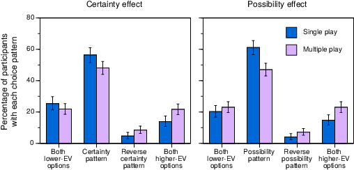
Figure 6: Percentages of participants with each of the possible choice patterns in problems related to the certainty and possibility effects in the standard conditions of our six within-participants studies. Error bars indicate 95% CIs, but these ignore between-study variability.

---

3.4  Unpacking the within-participants results

The above measures of certainty and possibility effects are based on the difference between the (logit-transformed) percentages of participants choosing the higher-EV option in two different problems. These measures are useful because they can be computed in both between- and within-participants designs. Unfortunately, however, a reduction in this measure of the certainty effect, for example, does not necessarily imply an equivalent reduction in the percentage of participants displaying the certainty choice pattern. To see why, one must consider the prevalence of three of the four possible choice patterns to the scaled-down, no-certainty problem (Problem 2) and the scaled-up, certainty problem (Problem 8): choosing both higher-EV options (HH%), choosing the higher-EV option in Problem 2 and the lower-EV option in Problem 8 (the certainty pattern, C%), and choosing the lower-EV option in Problem 2 and the higher-EV option in Problem 8 (the reverse certainty pattern, RC%). The fourth pattern, choosing both lower-EV options, is not directly relevant. The percentage of participants choosing the higher-EV option in Problem 2 is HH% + C% and the percentage choosing the higher-EV option in Problem 8 is HH% + RC%. The difference between these two percentages (the basis for our measure of the certainty effect in the preceding analyses) is thus C% – RC%. For this difference-based measure, a certainty effect is observed whenever there is a systematic imbalance between the two choice patterns. More important, any decrease in this measure in multiple play could be due to a decrease in C%, an increase in RC%, or a combination of changes (e.g., a larger decrease for C% than for RC%). Analogous logic applies to the possibility effect.

Within-participants designs are appealing in this context precisely because they provide this level of detail. Figure 6 shows the percentages of participants with each of the four possible choice patterns for problems related to the certainty effect (Problems 2 and 8) and, separately, for problems related to the possibility effect (Problems 4 and 10) in the standard conditions of our six within-participants studies. For simplicity, we have aggregated across the 10- and 100-play conditions in Studies 1 and 3, across the dollars and cents conditions in Study 4, and across studies (ns = 1027 and 1076 for the certainty and possibility effects, respectively). (Tables S.4–S.14 in the Supplement provide counts and percentages for all choice patterns separately for all conditions of all of our studies.)

The percentage of participants exhibiting the certainty choice pattern in Problems 2 and 8 dropped from 56.3% in single play to 48.1% in multiple play. Random-effects meta-analyses revealed that this reduction was significant for our data, overall b = 0.39, CI [0.06, 0.72], OR = 1.47, t(5) = 3.00, p = .030, and when Barron and Erev’s (2003) data were also included (total n = 1188), overall b = 0.49, CI [0.16, 0.82], OR = 1.63, t(6) = 3.61, p = .011 (for Barron & Erev’s data alone, the drop from 33% in single play to 10% in multiple play was significant, OR = 4.42, Fisher exact p < .001).¹⁵ In contrast to Barron and Erev’s results, the certainty pattern remained the modal choice pattern in multiple-play decisions in five of our six within-participants studies and was the majority pattern in Studies 1 and 3 (in Study 5, the modal pattern in multiple play was choosing the lower-EV option in both problems). In Problems 4 and 10, the percentage of participants exhibiting the possibility choice pattern dropped from 61.1% to 47.0% in our studies, overall b = 0.63, CI [0.29, 0.97], OR = 1.88, t(5) = 4.76, p = .005. The possibility pattern remained the modal pattern in multiple-play decisions in all six studies and was the majority pattern in Studies 1, 3, and 5.

---

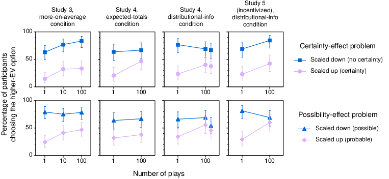
Figure 7: Percentages of participants choosing the higher-EV option in problems related to the certainty effect (top) and the possibility effect (bottom) in the long-run-prompt conditions of our Studies 3–5. In the distributional-info condition of Study 4, the results for 100 plays with cents appear to the right of those for 100 plays with dollars. Error bars indicate 95% CIs.

---

The prevalence of the reverse certainty pattern increased from 4.6% in single play to 8.4% in multiple play (see the left panel of Figure 6). This increase was nearly significant in our data, overall b = 0.66, CI [–0.18, 1.50], OR = 1.93, t(5) = 2.02, p = .099, and was significant when Barron and Erev’s (2003) data were also included, overall b = 0.80, CI [0.04, 1.57], OR = 2.24, t(6) = 2.58, p = .042 (for Barron & Erev’s data alone, the increase was from 7% to 24%, OR = 4.54, Fisher exact p =.003). For the reverse possibility pattern, the increase from 4.0% to 7.1% in our data was not significant, overall b = 0.47, CI [–0.42, 1.36], OR = 1.60, t(5) = 1.36, p = .23 (see the right panel of Figure 6).

Overall, the moderating effects of multiple plays were less impressive for common-ratio choice patterns than for common-ratio effects. For our studies, reductions in the prevalence of the certainty and possibility choice patterns (overall effect sizes of 0.39 and 0.63, respectively) were smaller than the corresponding reductions in the certainty and possibility effects (overall effect sizes of 0.82 and 0.99, respectively, for the same six studies). This difference reflects the fact that the prevalence of the reverse choice patterns increased in multiple play, though not significantly.¹⁶

3.5  Conditions designed to encourage a long-run perspective

In addition to the standard conditions discussed above, Studies 3–5 also included one or more conditions designed to push participants toward adopting a long-run view. In all, there were three long-run-prompt conditions, which we label the more-on-average, expected-totals, and distributional-info conditions (see the Supplement for details). As part of the more-on-average condition of Study 3, participants indicated whether they would make more money on average with Option A or Option B before they made a choice. Participants in the expected-totals condition of Study 4 estimated their expected total winnings over 100 plays of each option before they made a choice. In the distributional-info condition of Studies 4 and 5, participants were told the mean and 90% confidence intervals for total winnings over 100 plays of each option before they made a choice. For the more-on-average and expected-totals conditions, we reasoned that pushing participants toward more thorough and integrative processing, which has been shown to occur naturally in other multiple-play decisions (Joag et al., 1990; Su et al., 2013; Wedell & Böckenholt, 1994), might lead to greater reductions of common-ratio effects in multiple play. For the distributional-info condition, we reasoned that providing participants with relevant but difficult-to-estimate information about the outcome distributions might have an even stronger effect, analogous to that observed for decisions about mixed, positive-EV gambles (Benartzi & Thaler, 1999; DeKay & Kim, 2005; Klos, 2013; Langer & Weber, 2001; Redelmeier & Tversky, 1992).

Figure 7 displays results for all three long-run-prompt conditions. As expected, these conditions generally increased the percentage of participants choosing the higher-EV option and reduced the magnitudes of the certainty and possibility effects (see the Supplement for analyses). The important question for this article, however, is whether the effect of multiple plays on the magnitude of the certainty and possibility effects was moderated by the long-run prompts. Although one might expect that the effect of multiple plays would be enhanced in the presence of the prompts (or equivalently, that the effect of the prompts would be enhanced in multiple play, where the long-run view is generally considered more relevant; Camilleri & Newell, 2013; Li, 2003; Montgomery & Adelbratt, 1982; Wulff et al., 2015), this was not the case. In aggregate analyses that controlled for study (n = 900), the three-way Condition × Problem × Plays interaction was not significant for either the certainty effect or the possibility effect, both ps ≥ .29. Controlling for study, both the certainty effect and the possibility effect remained significant in multiple-play decisions in the long-run-prompt conditions, both ps < .001.

Separate analyses for the different studies and long-run-prompt conditions yielded similar results, though there was some variation. In particular, the possibility effect was eliminated in multiple-play decisions in the distributional-info condition of Study 5, McNemar exact p = .39, but the certainty effect remained strong in multiple-play decisions in the same condition of that study, p < .001 (see Figure 7). Curiously, these results were nearly the opposite of those in the standard condition of Study 5, where the certainty effect was not quite significant in multiple play, p = .064, but the possibility was, p < .001 (see Figures 1 and 2). Collapsing across the standard and distributional-info conditions of Study 5, both effects remained strong and significant in multiple-play decisions, both ps < .001.

Notwithstanding this variation, it appears that requiring participants to think about aggregate long-term outcomes (as in the more-on-average and expected-totals conditions) or telling them what those aggregate outcomes are likely to be (as in the distributional-info condition) is not generally sufficient for eliminating common-ratio effects in multiple-play decisions.

3.6  Individual differences in insight and numeracy

To assess the possible effects of more thorough and integrative processing in a different way, we also tested whether the effects of multiple plays were moderated by individual differences in insight and numeracy (see the Supplement for details). We defined high-insight participants as those who correctly identified the better option in the relevant problems of Study 3’s more-on-average condition and those who correctly ordered the expected payoffs of the options in the relevant problems of Study 4’s expected-totals condition. As anticipated, these high-insight participants were more likely to choose higher-EV options, all ps ≤ .001. However, there was no indication that high-insight participants showed significantly smaller certainty and possibility effects or that the effect of multiple plays on certainty and possibility effects was reliably different for high- and low-insight participants, all ps ≥ .14.

To investigate the possible effects of numeracy, we conducted combined analyses of the standard conditions of Studies 4–6, treating numeracy as a continuous measure and controlling for study. For the certainty effect, there were no significant effects of numeracy or its interactions, all ps ≥ .14. For the possibility effect, more numerate participants were more likely to choose higher-EV options, p < .001. Interestingly, more numerate participants exhibited larger possibility effects than less numerate participants in single-play decisions, p = .005, but not in multiple-play decisions, p = .38, though the three-way interaction that distinguishes these situations was not significant, p = .13. Finally, considering only those participants with above-average numeracy scores (five or higher on the eight-item scale), the certainty and possibility effects remained significant in multiple play, again controlling for study, both ps < .001. In summary, certainty and possibility effects in multiple-play decisions appear to be largely unrelated to participants’ insight and numeracy.

4  Discussion

Results from our primary meta-analyses indicated that, on average, certainty and possibility effects in multiple-play decisions were about 50–60% as large as those in single-play decisions. In other words, the effects were reduced but not eliminated (see Figures 4 and 5). With the exception of Study 6, the certainty-effect reductions in our studies were similar in magnitude to those in previous studies. However, because the certainty effects in the single-play conditions of our studies were larger than those in previous studies, these reductions were insufficient to eliminate the effects. For possibility effects, the reductions in our studies were noticeably smaller than that reported by Keren and Wagenaar (1987).

In our within-participants studies, reductions in the prevalence of the certainty and possibility choice patterns in multiple play were even smaller than the corresponding reductions in the certainty and possibility effects, because of the (nonsignificant) rise in the prevalence of the reverse choice patterns in multiple play (see Figure 6). Indeed, the certainty and possibility choice patterns almost always remained the modal or majority patterns in multiple-play decisions in our within-participants studies.

In general, the effect of the number of plays on the magnitude of certainty and possibility effects was not significantly moderated by (a) conditions designed to foster a long-run perspective, (b) participants’ insight into the expected long-run payoffs of the gambles in question, or (c) participants’ numeracy.

What is most surprising in our results — and what sets our results apart from those of previous studies — is how strongly participants clung to lower-EV options in multiple-play decisions. For example, in Problem 8 of the distributional-info condition of our incentivized Study 5, we told participants that they could expect to win 600¢ total with 100 plays of one option and about 800¢ total (with a 90% chance of winning between 730¢ and 860¢) with 100 plays of the other option. Despite this forceful push toward the higher-EV option, 26 of the 45 participants in this condition (58%) chose the lower-EV sure thing. Moreover, the percentage of participants exhibiting the certainty choice pattern (44%) was only slightly less than that for single-play decisions in the same information condition (48%).

It is possible that we could eliminate common-ratio effects in multiple-play decisions by using even stronger information manipulations. For example, we could show participants the complete distributions of possible aggregate outcomes or we could tell participants the exact likelihood of coming out ahead in the long run with one option or the other (e.g., that there is a 99.9996% chance that the total payoff from 100 plays of the risky option will exceed the total payoff from 100 plays of the certain option in our Problem 8). However, the potential benefit of such efforts is unclear, especially when previous studies have eliminated common-ratio effects without providing any additional information to participants.

4.1  Why the discrepancy in persistence?

The obvious question is why the certainty and possibility effects persisted in multiple-play decisions in our studies, but not in previous studies. Differences between gambles is not a plausible explanation, as we based our gambles on those used by previous authors (Keren, 1991; Keren & Wagenaar, 1987, Study 2). Differences in motivation or ability between our U.S. participants and previous authors’ Dutch and Israeli participants also strike us as unlikely explanations. Individual differences in insight and numeracy did not significantly affect our primary results, nor did our attempts to promote participants’ long-run insight with various prompts. A third, more general observation — that effect sizes tend to be smaller in replications than in the initial research (Open Science Collaboration, 2015) — applies to our results, but only partially. Although the effect of multiple plays on the possibility effect was smaller in our studies than in previous work (see the right panel of Figure 5), this was not generally the case for the certainty effect (see the right panel of Figure 4). Additionally, the certainty and possibility effects themselves remained larger in the multiple-play conditions of our studies than in previous research (see the middle panels of Figures 4 and 5).

Another potential reason for the discrepancy is that we usually assessed certainty and possibility effects within participants, whereas Keren and Wagenaar (1987) and Keren (1991) assessed them between participants. For the certainty effect, this explanation is clearly contradicted by the evidence. For example, the largest reduction and the smallest certainty effect in multiple play (indeed, a nearly significant reverse certainty effect) were reported by Barron and Erev (2003), who used a within-participants design. Keren’s (1991) design also had within-participants features (see footnote 11). Additionally, the certainty effect remained significant in multiple-play decisions in our between-participants Study 2 (see Figure 1) and our between-participants analyses of Studies 1 and 7 (see Figure 3), all Fisher exact ps ≤ .001. The verdict is less clear-cut for the possibility effect. That effect was not significant in multiple-play decisions in our between-participants Study 2, Fisher exact p = .21 (see Figure 2), but it remained significant in our between-participants analyses of Studies 1 and 7, p < .001 and p = .036, respectively (see Figure 3). Interestingly, the reduction of the possibility effect in Studies 2 and 7 resulted from a smaller percentage of participants choosing the higher-EV option in the scaled-down problem rather than (or in addition to) a larger percentage of participants choosing the higher-EV option in the scaled-up problem. That is not the pattern of results observed by Keren and Wagenaar (1987, Study 2). More formal analyses using all studies indicated that the within- versus between-participants distinction did not significantly moderate the certainty effect or the possibility effect in multiple-play decisions, both ps ≥ .21 (see the Supplement for details and cautions).

4.2  A few thoughts about cognitive processes

Although the primary goal of our studies was not to distinguish between common-process and different-process explanations for the moderating effects of multiple plays (Wedell, 2011), some of our conditions and analyses were guided by those explanations, at least in a general way. If multiple-play decisions naturally lead some participants to think about aggregate long-run outcomes, as previous research suggests, then pushing participants in that direction (as in our more-on-average and expected-totals conditions) or telling them what those aggregate outcomes are likely to be (as in our distributional-info condition) should have led more participants to think in that manner, or to think in that manner more clearly. In other words, if one views “thinking about long-run outcomes” as a potential mediator of the effect of multiple plays on choosing higher-EV options, then one can also view our long-run-prompt conditions as attempts to manipulate that mediator. On the one hand, these manipulations performed as expected: They increased the popularity of higher-EV options and reduced the sizes of the certainty and possibility effects, providing at least some support for the role of outcome aggregation in the reduction of common-ratio effects. On the other hand, these changes were rather limited and were not significantly more pronounced in multiple play than in single play (compare the panels of Figure 7 to the corresponding panels of Figures 1 and 2). Apparently, directing participants to consider aggregate outcomes is not enough to eliminate common-ratio effects in multiple-play decisions.

Though not eliminated, common-ratio effects were reduced in multiple play, even in our standard conditions. Participants were more likely to chose the riskier, higher-EV option in multiple play than in single play when considering scaled-up problems, but this was not generally true for scaled-down problems (see Figures 1 and 2). These interactions are interpretable in terms of psychological processes, at least in principle (Loftus, 1978; Wagenmakers et al., 2012). As noted in the introduction, however, there is little agreement regarding the processes underlying common-ratio effects or the effects of multiple plays. Even so, some of our participants surely considered the implications of multiple plays for the riskiness of the two options, the likelihood of coming out ahead with either of the two options, or some other relevant comparison. For example, risk decreases as the number of plays increases, at least for one psychologically relevant measure of risk (the coefficient of variation; Klos et al., 2005; Weber, Shafir & Blais, 2004). As a result, participants may have been more likely to choose the riskier, higher-EV option because it seemed less risky in multiple play than in single play, even if they were not less risk averse in multiple play. This shift toward choosing the higher-EV option may have been larger in scaled-up problems than in scaled-down problems because there was more room for an increase in scaled-up problems (see Figures 1 and 2), because the risk reductions separated the options better in scaled-up problems (see the first section of the Supplement for a related discussion), or for other reasons. According to this logic, multiple plays might reduce common-ratio effects not because participants behave more rationally, but because the risk reductions associated with multiple plays reduce the tension between risks and payoffs, making the condition poorly suited to detecting common-ratio response patterns (relative to single play).

Perhaps the most parsimonious explanation for the persistence of common-ratio effects in our studies is that many participants did not think seriously about the implications of multiple plays, even when those implications were spelled out. Instead, participants making multiple-play decisions may have employed the same decision strategy (or a similar mix of decision strategies) as participants making single-play decisions, without much regard for distributions of aggregate outcomes. But why would participants not consider the implications of multiple plays? One plausible answer comes from Weber and Chapman (2005, Study 3), who reported that the certainty version of the common-ratio effect was not significantly reduced when the outcomes of the gambles in each choice would be delayed by 25 years, even though the delay introduced a form of uncertainty. Apparently, their participants treated the delay as a common attribute that did not distinguish between the alternatives and therefore ignored or edited out that information when choosing between them. Many of our participants may have treated the number of plays analogously, thus overgeneralizing a useful simplification strategy to a situation in which it should not be applied. However, even if this overgeneralization is considered defensible in our standard conditions, it is clearly not defensible when the implications of multiple plays are made transparent, as they were in the distributional-info condition of Studies 4 and 5. Moreover, we have no good explanation for why participants would use such a strategy in our studies but not in other researchers’ studies.

Finally, the frequency of reverse common-ratio choice patterns was slightly higher in the multiple-play conditions of our studies and was significantly higher in the multiple-play condition of Barron and Erev’s (2003) study. One relatively straightforward explanation for such increases is that multiple-play decisions are more complicated than single-play decisions, making it harder for some participants to identify the higher-EV option. The resulting increase in noise could partially offset the improved decision making of other participants. Given their reliability in other studies (Blavatskyy, 2010; Nebaut & Dubois, 2014) and their role in the estimation of common-ratio effects, reverse common-ratio choice patterns warrant further attention.

To recap, we speculate that participants may react to multiple-play decisions in three general ways. First, they may realize that having many plays helps differentiate the two options and then determine or intuit that they would be better off choosing the (not terribly risky) higher-EV option. Second, they may instead ignore the number of plays because they think, incorrectly, that this common attribute does not help differentiate the options. Such participants would respond as if they were in single play. Third, they may try to think through the implications of multiple plays but be unable to do so. Participants in this group might give up and respond as if they were in single play or they might respond more randomly (or in ways that appear more random) in the face of this increased uncertainty. If there are enough participants in the first category, experimental results will look like those of Keren and Wagenaar (1987) and Keren (1991); if there are more in the second and third categories, the results will look more like ours.

4.3  Putting the results in context

Although our finding that common-ratio effects are not eliminated in multiple play is at odds with previous results for these effects, it is consistent with the broader literature on the distinction between single- and multiple-play decisions. For example, when the distribution of possible aggregate outcomes is not shown, the percentage of participants opting to play mixed, positive-EV gambles usually increases in multiple play, but the increases are far from complete (e.g., from 43% to 63% in Redelmeier & Tversky, 1992) and are not always observed (e.g., Benartzi & Thaler, 1991, Study 1). Similarly, Liu and Colman (2009) reported that the percentage of participants choosing an ambiguous, higher-EV option over an unambiguous, lower-EV option increased in multiple play, but 29% to 49% of participants (depending on the study and choice) still sacrificed EV in order to avoid ambiguity. The description-experience gap is also not eliminated in multiple-play decisions, though it is reduced (Camilleri & Newell, 2013).

Wedell and Böckenholt (1990) reported that preference reversals were eliminated in the 100-play condition of their Study 2, though not the 10-play conditions of their two studies. Because of the design of those studies, there are strong parallels with our within-participants studies. As in our analyses of common-ratio effects, Wedell and Böckenholt’s results were based on percentage differences that depended on the relative frequencies of two different response patterns (preference reversals in the typical, predicted direction¹⁷ and preference reversals in the opposite direction), as those authors noted. Analogous to our results, the frequency of the predicted preference-reversal response pattern decreased with multiple plays in both studies, but the frequency of the opposite response pattern increased in both studies. In the 100-play condition of their second study, the predicted and opposite preference reversals accounted for 24% and 16% of response patterns, respectively. The authors’ conclusion that “preference reversals … were effectively eliminated” (p. 434) in that condition means only that the asymmetry between those percentages (i.e., the 8-percentage-point difference) was not significantly different from zero, not that the percentage for the predicted preference reversal (24%) or the total percentage for both types of preference reversal (40%) was close to zero. In other words, the preference-reversal effect was eliminated, but the preference-reversal response patterns were alive and well.

By extension, when common-ratio effects are not significant in the multiple-play conditions of between-participants studies like Keren and Wagenaar’s (1987), Keren’s (1991), and our Study 2, this result tells us only that the asymmetry between the (assumed but unmeasured) common-ratio choice pattern and the reverse choice pattern is not significant. It does not tell us very much about the prevalence of the common-ratio choice pattern itself, though that prevalence is (by definition) at least as large as the prevalence difference between the two choice patterns. This distinction between effects and choice patterns is by no means novel, but its importance for the interpretation of results remains underappreciated. In our view, research on judgment and decision making would benefit from greater attention to the response patterns of individual participants and the variation in such patterns across participants and conditions.

To summarize, the most common result in this literature is that violations of EV and EU theories are reduced but not eliminated in multiple-play decisions. Viewed against this backdrop, the persistence of common-ratio effects in multiple-play decisions in our studies seems less surprising than the comparisons to previous studies in Figures 1 and 2 suggest.

5  Conclusions

In terms of the number of participants, the seven new studies reported in this article more than double the amount of data on the effect of multiple plays on the certainty effect. For the possibility effect, the increase in data is more than fivefold. Considering all of the available evidence, both of these common-ratio effects are reliably reduced when participants consider playing the relevant gambles multiple times. Yet despite these reductions, both effects remain significant and reasonably large in multiple-play decisions, at least on average. The latter result suggests that the oft-cited beneficial effects of multiple plays on the rationality of decision makers’ choices may be weaker than previously realized. Although multiple-play decisions are often different from — and arguably better than — single-play decisions, well-established biases are unlikely to disappear completely in multiple-play decisions.

References

*

Department of Psychology, The Ohio State University, 1835 Neil Avenue, Columbus, OH 43210. Email: dekay.3@osu.edu.

#

Department of Social and Decision Sciences, Carnegie Mellon University

Dan R. Schley is now at Department of Marketing Management, Rotterdam School of Management, Erasmus University, Rotterdam, The Netherlands. Jonghun Sun is now at Root Impact, Seoul, Korea. Michael N. Karim is now at Fors Marsh Group, LLC, Arlington, Virginia. Funding for Studies 1 and 2 was provided by National Science Foundation grant SES–0218318. We are grateful to Megan French, Rachael Martin, Elena Reynolds, and David Wanner for assistance conducting Studies 3–5 and to Hal Arkes, Tomás Lejarraga, Amanda Montoya, Ben Newell, and Dirk Wulff for their insightful comments on earlier versions of this manuscript. The first author wrote the initial version while a visiting researcher at the Center for Adaptive Rationality at the Max Planck Institute for Human Development in Berlin, Germany.

Copyright: © 2016. The authors license this article under the terms of the Creative Commons Attribution 3.0 License.

1

We follow Camilleri and Newell (2013; and also Chen & Corter, 2006) in distinguishing between multiple-play and repeated-play situations, though we recognize that these terms have been used interchangeably in the past. In Camilleri and Newell’s usage, a typical, binary multiple-play situation involves a single decision about a gamble (or a choice between two gambles) that will be played many times, with the same choice applying to all plays. A repeated-play situation, on the other hand, involves a string of identical single-play decisions in which the decision maker can make a different choice for each play. Although these two situations are clearly related, they are empirically different (Camilleri & Newell, 2013), in part because people do not naturally aggregate possible outcomes over a series of plays (Gneezy & Potters, 1997; Redelmeier & Tversky, 1992; Thaler, Tversky, Kahneman & Schwartz, 1997). Multiple-play and repeated-play decisions are normatively different as well, because the latter variety involves the option of changing one’s choice partway through the sequence. Aloysius (2007) noted that past disagreements regarding rationality in Samuelson’s (1963) famous example (which involved a person declining one play but accepting 100 plays of a 50:50 gamble for $200 or –$100) can be attributed in part to Samuelson’s treating a multiple-play situation as if it were a repeated-play situation. Chen and Corter also noted this discrepancy. In the present article, we are primarily concerned with (a) descriptive rather than normative issues and (b) multiple-play rather than repeated-play decisions.

2

That common-ratio and reverse common-ratio choice patterns violate EU theory in single-play decisions does not necessarily imply that they do so in multiple-play decisions. To our knowledge, this question has not been addressed previously. Our initial analyses (see the Supplement) indicate that reverse common-ratio choice patterns can be consistent with EU theory in multiple play for some utility functions in the power family (Wakker, 2008). However, in our limited explorations of decision problems from Kahneman and Tversky (1979), Keren and Wagenaar (1987), Keren (1991), and Barron and Erev (2003, Study 5), we found no cases in which standard common-ratio choice patterns are consistent with EU theory in multiple play.

3

This definition does not properly capture common-ratio effects in problems with equal-EV options (e.g., Kahneman & Tversky’s, 1979, Problems 7 and 8) or common-ratio effects in the domain of losses, where risk preferences are often reversed (Kahneman & Tversky, 1979; Keren & Wagenaar, 1987, Study 1), but it is sufficient for our purposes. Also, we note that Kahneman and Tversky did not use the term possibility effect. Keren and Wagenaar used the term for a common-ratio effect in which the scaled-down problem involves very small probabilities, but we don’t know if they were the first to do so. More recently, Kahneman (2011) used the term to refer to the overweighting of low-probability events. In this article, we follow Keren and Wagenaar’s usage.

4

Barron and Erev’s (2003) article focused almost entirely on decisions from experience rather than the more commonly studied decisions from description (for more on the distinction, see Hertwig, 2015; Hertwig & Erev, 2009). However, their Study 5 involved only decisions from description.

5

In Kahneman and Tversky’s (1979) Problem 7 (the scaled-up problem in their possibility-effect example), 86% of participants chose a 90% chance of 3000 Israeli pounds over a 45% chance of 6000. However, assuming Tversky and Kahneman’s (1992) parameter values, the cumulative-prospect-theory value for the former option (817) is less than that for the latter option (835), as can be verified here: http://prospect-theory.behaviouralfinance.net/cpt-calculator.php. As a result, the 1992 parameter values imply consistent choices in the scaled-up and scaled-down problems, and hence no possibility effect. This prediction conflicts with the 1979 finding.

6

In the multiple-play version of Problem 2 (the scaled-down, no-certainty problem) in Studies 1, 3, 4, and 5, the phrase “on each gamble” appeared after the word “that” rather than before it. Although this unintended wording could have changed participants’ interpretations and hence their choices, there is no indication that it did. Choice proportions for this problem were very similar to those in Studies 2, 6, and 7, which used the intended wording (see Figure 1 in the Results section). All other problems used the intended wording.

7

Keren (1991) used a somewhat similar procedure, though payoffs in the multiple-play (5-play) condition were not reduced and only one participant from each group of 8 to 12 was paid.

8

We used SAS PROC GENMOD regardless of whether problem was varied between or within participants. When there was more than one observation per participant, GENMOD used generalized estimating equations that yielded population-average estimates. Conceptually, these estimates are more comparable to those from completely between-participants studies than are the average unit-specific (participant-specific) estimates from random-effects models. Although population-average and unit-specific estimates typically differ for nonlinear models (Hu, Goldberg, Hedeker, Flay & Pentz, 1998; Raudenbush & Bryk, 2002, pp. 303–304), random-effects models fit using SAS PROC GLIMMIX yielded identical or nearly identical results in our studies.

9

Results were similar when we used orthogonal contrast codes to distinguish the three levels of the plays variable. Specifically, the first code compared the 1-play condition (coded –2/3) to the 10- and 100-play conditions (coded +1/3), whereas the second code compared the 10- and 100-play conditions (coded –1/2 and +1/2, respectively) while ignoring the 1-play condition (coded 0). The first code yielded results much like those in our primary analyses. For the second code, neither its main effect nor its interaction with problem was significant in either analysis (for certainty or possibility effects), all ps ≥ .40. Similar results were obtained for the second code in Studies 2 and 3 (the only other studies with both 10- and 100-play conditions), all ps ≥ .072. Of the six possible interactions involving the second code in Studies 1–3, only three had the anticipated negative sign (see Figures 1 and 2). Thus, the distinction between 10 and 100 plays did not have a reliable effect on certainty and possibility effects in our studies.

10

Greg Barron (personal communication, 2003) provided the data for Barron and Erev’s (2003) Study 5 (see Table S.3 in the Supplement).

11

Keren’s (1991) experimental design involved two parallel (i.e., similar, but not identical) sets of gambles. For single play (n = 49), some participants received the certainty problem (like our Problem 8) from one set and the no-certainty problem (like our Problem 2) from the other set, whereas others received the reverse. A similar procedure was used for multiple play (n = 47). Because different participants received the certainty and no-certainty problems in each set, Keren treated problem as a between-participants variable. We also analyzed Keren’s study in this way. However, because Keren collapsed across the two parallel sets of gambles, each participant contributed two choices, doubling the sample size for the relevant statistical tests (e.g., the number of observations in Keren’s Table 1 is 192, twice the true N of 96). To address this sample-size issue (but not the related independence issue), we divided the counts in Keren’s Table 1 by two. Because doing so yielded some noninteger counts, we conducted our analysis twice, once with counts rounded up and once with counts rounded down, and then averaged the results. This procedure increased the standard errors of the logistic regression coefficients (relative to those for N = 192), but otherwise had no effect on our substantive results. Though imperfect, this solution is preferable to omitting the study from our meta-analysis.

12

Rescaling the effect sizes to express them in a common metric, as suggested by Morris and DeShon (2002) for standardized effect sizes arising from within- and between-participants studies, is not necessary in our case because we use unstandardized regression coefficients from otherwise identical models.

13

In random-effects meta-analysis, the overall effect size is an estimate of the mean of a distribution of population effect sizes rather than an estimate of a single population effect size (Shadish & Haddock, 2009). The random-effects model reduces to the fixed-effect model when the between-study variance is estimated to be zero. We report results from random-effects meta-analyses, but fixed-effect meta-analyses yielded similar conclusions.

14

For each study, the third effect size is equal to the difference between the first two. However, this is not exactly true for the overall effect sizes, presumably because the relative weighting of the studies (which is based on the inverses of the variances of the studies’ effect sizes) differs somewhat in the three analyses.

15

For consistency with our other meta-analyses, these reductions are written as positive effects. Also, because these within-participants studies had essentially identical designs, we used individual participant data rather than aggregated data for these meta-analyses (Cooper & Patall, 2009).

16

For percentages, the relationships between effects and choice patterns are dictated by simple arithmetic. This is not true for the corresponding effect sizes, however, presumably because of the logit transformation and the vagaries of fitting random-effects models.

17

The typical preference-reversal response pattern was that participants preferred the gamble with a higher probability of winning a smaller amount (the P bet) when choosing between two gambles, but preferred the gamble with a lower probability of winning a larger amount (the $ bet) when pricing the gambles.

This document was translated from L^AT_EX by H^EV^EA.