 Figure 1: Strong-lexicographic answering in the Dutch surveys.
Judgment and Decision Making, Vol. 12, No. 3, May 2017, pp. 260-279
Establishing the relevance of non-compensatory choice algorithms from stated choice surveys – an explorationEvert Jan van de Kaa* |
In applied sciences large-scale surveys are a popular means to acquire insights in the choices that people make in different contexts. In transportation research, for example, tens of thousands stated their choices between alternatives characterized by cost and time attributes. In this study I explore the extent to which the data acquired in such studies may exhibit the co-occurrence of different choice algorithms within such survey populations. For that purpose I propose a novel version of the outcome-oriented approach. It is applied to the outcomes of two Dutch value-of-time surveys. If the recorded choice patterns are viewed apart, most could be the result of several different algorithms, in line with the main criticism of the outcome-oriented approach. The novel version considers the causal relationships between an individual’s personal circumstances, his use of a particular algorithm and the resulting choice pattern. It employs inferential statistics for analyses of the frequencies of the expected and actually recorded choice patterns within groups of respondents. Applied to the Dutch survey results this allowed disentangling, at the aggregate level, the overlap in explaining compensatory and non-compensatory algorithms to a large extent. It revealed that weighted additive (WADD) algorithms incorporating different degrees of loss aversion could explain most recorded choice behaviour while none of the many non-compensatory algorithms that were considered yielded a more than marginal explanation. Replications of this study, preferably by re-analysing other large-scale surveys with more complicated choice sets, is recommended to find out whether or not these findings are incidental.
Keywords: outcome-oriented approach, non-compensatory decision
rule, lexicographic rule, Elimination-by-Aspects, random choice, human
error, value of time, loss aversion
In applied sciences like transportation research and environmental science, large-scale choice surveys are a popular means to acquire insights in the values that people attribute to changes in their circumstances. In transportation research, for example, the value that travellers assign to travel time savings (VTTS) is of utmost importance for infrastructure management and planning. For that reason national VTTS surveys are performed every now and then in many countries (e.g., Burge, Rohr, Vuk & Bates, 2004). Most VTTS-survey designs are similar and the choice sets simple: two trip alternatives, each characterized by two attributes: travel time and travel cost. These games are embedded in questionnaires asking dozens of questions about socio-economic and travel-context-related personal characteristics, though commonly observations about the respondents’ choice processes are missing. In the Netherlands alone, between 1988 and 2011 about 15,000 travellers participated in such surveys. Worldwide, more than a hundred thousand people did so in these and similar stated choice studies (e.g., Van de Kaa, 2010a).
Mostly such large-scale surveys are made to acquire data for the estimation of the parameters of models meant for prediction of choice behaviour in similar real-life circumstances. The aim of the current study is to explore whether or not the raw data from such surveys can be used for estimating the distribution of different explanatory choice algorithms1 over segments of the survey population. Understanding of this is important, as different algorithms may imply different transferability requirements from estimation to prediction contexts. To be precise, I will examine the extent to which non-compensatory algorithms, if added to a mixture of compensatory algorithms, may increase a model’s explanatory ability.
For this study, a novel version of the outcome-oriented approach2 was developed. Section 2 motivates and outlines this “outcome-oriented inferential statistics” — approach. In Appendix 1 it is tested on some imaginary survey outcomes. By courtesy of Rijkswaterstaat the full documentation of the Dutch 1988 and 1997 national VTTS surveys was made available for the current research. Section 3 overviews the designs of these surveys and offers a preliminary analysis of the choices that were recorded. Section 4 examines the extent to which several algorithms that comply with WADD (Payne, Bettman & Johnson, 1993) would yield these outcomes. It shows that such algorithms, particularly those accommodating loss aversion, might explain by far most. In sections 5 and 6 the applicability of outcome-oriented inferential statistics is tested on the Dutch survey data. It appears that a bunch of lexicographic and attribute-threshold-based algorithms add hardly anything to the explanation of the recorded choice behaviour. The article finalizes with a discussion, summary, conclusions and recommendations concerning the relevance of these findings and the usefulness of outcome-oriented inferential statistics.
This section shortly reviews the main choice-algorithm-elicitation approaches from applied sciences and psychological research, and their limitations. It shows that an outcome-oriented approach is the way to go for the present study. The proposed version of this approach focusses on statistical analyses of predicted versus recorded choice patterns and draws on the assumed causal relationships between the individuals’ circumstances and their context-dependent choices.
In most applied work on stated choice, choice algorithms are used as explanatory-behavioural models (e.g., Hoffman, 1960). From that stance it is irrelevant whether people perform calculations deliberately or unconsciously or use simplifying heuristics or their memory, as long as they arrive at a similar choice as predicted by the model (e.g., Friedman, 1953). No matter how, consumers are presumed to maximize their utility by choosing the alternative for which the sum of the values (utilities) of all attributes is highest. For analyses of stated choice surveys, Random Utility Maximization (RUM) is a de facto standard in most branches. With very few exceptions the WADD rule is assumed for the assessment of the alternatives’ utilities (e.g., Foerster, 1979; McFadden, 2001). This is complemented with variables that relate to the decision-maker’s contextual and socio-economic characteristics and an error term that allows for stochastic interpersonal variations in tastes. For the latter, logit models are popular. These and similar discrete choice models are estimated by assessing mean parameters that offer the best fit between predicted and recorded choices of a survey population.
Such analyses that pre-assume WADD for each respondent do not allow inferences about the occurrence of the other choice algorithms that some of the consumers, or even most of them, may actually use. Moreover, Ballinger and Wilcox (1997) warned that the best-fitting parameters can be biased by the error specifications that are imposed. For example, a Gumbel-distribution across alternatives and individuals is assumed if a multinomial logit model is estimated but my scan of a few hundred applications in travel choice studies yielded none that reported its empirical confirmation. These cautions also hold for the occasional studies in which a non-compensatory rule or value function according to, e.g., Prospect Theory instead of utility maximization, is accommodated in a discrete choice model (e.g., Swait, 2001; Cantillo & Ortúzar, 2005; Ramos, Daamen & Hoogendoorn, 2013). Such RUM-models thus provide little if any information about the different choice algorithms that different respondents might have used in the same choice context.
The discovery of choice algorithms has been a major research topic in psychological research of human judgment and decision-making. (See Riedl, Brandstätter & Roithmayr, 2008, for an overview of some of these algorithms.) The two main methodological approaches in this field are process-tracing and the outcome-oriented approach (e.g., Rieskamp & Hoffrage, 1999; Glöckner, 2009). Apparently, inferring the use of particular decision rules by combining outcome-oriented and process-tracing techniques is state-of-the-art (Glöckner, 2009; Glöckner & Bröder, 2011; Hilbig, 2014). Process-tracing techniques “were developed to directly uncover the cognitive processes that take place between the onset of a stimulus and the decision maker’s response” while “in the structural-modelling paradigm, decision behaviour is investigated by fitting mathematical models to the relation between the attribute values of options (input) and the final response (output)” (Riedl et al., 2008, p. 795). Process-tracing is not useful in the present study as the required information is rarely if ever collected in large-scale surveys. But the inputs and outputs of the stated choice games are the core of the information that is collected. Thus, the outcome-oriented approach is necessary for the current research.
The main criticism of this approach is that different algorithms often explain the same choice observations (e.g., Montgomery & Svenson, 1989; Riedl et al., 2008; Glöckner, 2009; Bröder, 2010; Glöckner & Bröder, 2011). This problem may partly explain why I found no studies in experimental psychology in which the distribution of possibly co-occurring algorithms over survey populations was investigated extensively. Another explanation may be that the commonly small and homogeneous survey populations (e.g., students or scientific staff) in experimental psychology will often make a convincing statistical underpinning of inferences about such distributions problematic.
For my approach I borrowed from Bröder’s (2010) outcome-based-strategy-classification method. Obviously, his smart advice on survey design is not applicable here. But I not only start with the selection of choice algorithms that are plausible in the considered survey context (as he suggests) but also: assume consistent, though not necessarily error-free, application of these algorithms; predict the individuals’ choices with each considered algorithm; and compare this with the recorded ones in order to find one out of a group of tested algorithms that offers the best description of what the respondents’ mental processes do with the submitted attribute levels. In Systems Theory, Management Science and similar fields, this information-transformation system would be called the function of choice behaviour, see Van de Kaa (2008, ch. 2) for an extensive systems-theoretical view on human choice behaviour. Thus far, my approach differs in one respect from the usual outcome-oriented analyses in judgment-and-decision-making studies: the “objective” levels of the attributes, as submitted to the respondents, rather than their values to the respondents, are conceived as stimuli/input (e.g., Payne et al., 1993; Riedl et al., 2008). This approach implies that attribute appraisal/valuation is considered as inextricably bound-up with the choice process.
Another difference between the novel and common outcome-oriented approaches is that the sets of the individuals’ choices are the basic target of analysis, instead of their separate choice decisions. Following Van de Kaa (2006) I call such a set a choice sequence, which I will further denote as CS. When a person makes choices from c sets each containing a alternatives, he generates one out of ac theoretically feasible CSs. In my approach the frequencies of occurrence of the actually recorded CSs in a survey population are compared with those following from application of the considered algorithms.
If this approach is applied to an individual’s context-dependent set of choice decisions and yields different choice algorithms that can explain them, there is little hope to disentangle the overlap. Imagine, for example, a fictitious survey with n respondents who state their choices from the same five choice sets with each two alternatives. Further imagine that each respondent applies one out of three choice algorithms consistently: always selecting the left-side alternative; always selecting the cheapest alternative; and at random selecting any alternative. Now consider that three choice algorithms are deemed plausible in this survey: an inertia-driven left-side-preference rule, a budget-constraint-driven lexicographic preference for the cheapest alternative, and an inertia-driven random rule (Johnson, Payne & Bettman, 1993). Now, a respondent who systematically selects the alternatives presented at the left side of the questionnaire may exhibit either a left-side preference or the random rule; one who systematically marks the cheapest alternatives may have a lexicographic preference for it or, again, have applied the random rule. For these individuals both considered algorithms explain their CS. But statistical analyses of the recorded CSs, taken into account the rationales behind the use of different algorithms, can shed light on the distribution of these algorithms within the population. See Appendix 1 for an elaboration of the simple, fictitious choice setting sketched above and some examples of inferential statistical analyses. Appendix 1 also illustrates the increasing discriminatory power of inferential statistics with increasing survey population size.
Most choice algorithms that have been proposed assume causal relationships between the individuals’ personal circumstances3 and their context-dependent choices. I traced such rationales behind the different compensatory and non-compensatory algorithms that are discussed in this article and considered why different subpopulations of the Dutch respondents may have used these algorithms when assessing their choices. I employed the findings in statistical analyses for investigating the co-occurrence of WADD, random-choice, lexicographic and threshold-based algorithms. This appeared a powerful tool to discriminate between these explanatory choice algorithms.
Outcome-oriented inferential statistics may also be used to estimate the character and frequency of human error. In an ongoing research on the extent to which random errors – slips and mistakes (Norman, 1981; Reason, 1990) – may have biased the underlying choice statements of the Dutch surveys I found, for example, that slips following a binomial distribution across choice sets and respondents can explain very few once or twice recorded CSs. As this goes beyond the scope of the present study the underlying analyses are not reported here. In this article I applied all considered choice algorithms in a deterministic way. One reason to do so is the peculiar distribution of the CSs recorded in the Dutch surveys (see next section). The other is that so far I found no way to discern between the CSs biased by mistakes from those following from a consistently and perfectly applied choice algorithm. I have to admit that the latter argument was decisive in considering deterministic instead of stochastic choice algorithms. As a consequence, I may have inferred some CSs incorrectly as the result of a particular choice algorithm instead of being caused by mistakes in other algorithms. The frequencies of the algorithms that explain the most frequently reported CSs will thus be underestimated. A subordinate advantage of a deterministic specification is that it prevents faulty choice-algorithm distributions that may be found when imposing improper error specifications.
Table 1: Choice sets as submitted in the Dutch 1988 and 1997 VTTS surveys,
Alternative 1: decrease in Alternative 2: decrease in
alt. 1 choices
This section sketches the outlines of these surveys and provides a global statistical analysis of the respondents’ CSs. It appears that less than 1% of the feasible CSs accounted for over 80% of all responses. At first sight this suggest that by far most respondents applied one out of a few choice algorithms consistently to all choice sets, while few of them made random errors, exhibited random taste variations or used mixtures of algorithms and/or unusual ones.
The designs of the 1988 and 1997 surveys were the same. Car drivers, train and transit passengers were recruited while they were “on their way” for business, commuting or other purposes. They were asked on the spot to answer questions about their actual trip, e.g., origin-destination, motive and expected travel time. Those who agreed to participate in a postal survey received a customized questionnaire, summarizing the information collected in the recruitment interview and allowing corrections to this. The questionnaire asked for information about the recruitment trip, such as refund of costs, arrival time and delays, and about personal and household characteristics (e.g., gender, employment, income, …). It included twelve two-option choice sets, which I will denote here as SC1 … SC12. Each submitted alternative was characterized by two attributes only: travel time, with levels presented in minutes (min), and travel cost, with levels in Dutch guilders (Dfl). Both travel time and cost were indicated by increases and decreases compared to those of the trip on which the respondent was recruited. Choice sets SC1 to SC4 contained the recruitment-trip-levels alternative next to either a time-loss-and-money-gain or time-gain-and-money-loss alternative, and SC8 contained a dominant alternative. The cost levels submitted in 1988 and 1997 were identical in nominal terms. As the Dutch guilder inflated by app. 25% between the two surveys, in real money the 1997 cost levels were 80% of those in 1988. There were different questionnaires for four recruitment-trip-duration classes. These questionnaires differed chiefly in the absolute scale extensions of the attributes. Table 1 lists the choice sets. For ease of understanding, the alternatives are recoded such that any consistently trading respondent with a sufficiently high VTTS would prefer alternative 1 over 2: in the stated choice sets SC1, 4, 6, 8, 9 and 12 alt. 1 was submitted at the left side of the questionnaire and alt. 2 at the right side; in the remaining sets this was reversed.
The documentation of these surveys includes the tabulated responses of all respondents. The 1997 files comprised corrections, by several respondents, on the information collected in the recruitment interview, which were not yet processed. After processing, 30 questionnaires appeared not useful, mostly because the travel mode in the questionnaire differed from the recruitment trip. After exclusion of these, and 630 more in which one or more SC questions were not completed, 7147 questionnaires remained for analyses in the current study. For extensive descriptions of the surveys, including examples of the employed questionnaires, response rates, and distribution and impact of socio-economic and trip-related characteristics on recorded choice behaviour, see HCG (1990, 1998).
From first principles as well as empirical studies it is well-established that wealth and free time4 are very important indicators of people’s monetary value of travel time (e.g., DeSerpa, 1971; Gunn, 2001; Jara-Díaz & Guevara, 2003; Van de Kaa, 2010c). As a proxy of wealth, the questionnaire asked the participants to report their household income. It also solicited information about the time spent for paid labour, obligatory travel and housekeeping. I enriched the time-spending information by adding estimates for uncompleted questions, time for other obligatory activities (study) and for personal activities (sleeping, eating, and personal care). To that end I interpolated the average time spending, differentiated according to gender, age, education and occupation, as reported in the 5-yearly Dutch national time-use surveys (Van den Broek et al., 2004), to arrive at 1988 and 1997 data. These estimates of respondent-specific obligatory and personal time thus took their reported socio-economic characteristics into account. The respondents’ free-time budgets were found by subtracting these estimates from the total time per week.
As explained in the previous section, the complete set of each individual’s choices made in the elicitation context, termed CS, is my basic target of analysis. For the Dutch surveys, with a = 2 alternatives in c = 12 choice sets, there are ac = 4096 different feasible CSs. To denote particular CSs I ordered the numbers of the chosen alternatives from SC1 to SC12 in a 12-digit number. For example, the succession of choices that follows from systematic choice for the left-side alternative (column 6 of Table 1) yields 122 121 211 221. In the Data (linked from the journal’s table of contents) the answers of all 7147 respondents to the 12 SC questions are listed, together with the corresponding CSs, the scale extensions (see Section 6) of the choice sets submitted to them, and their household income and free time.
Table 2: Recorded occurrence of choice sequences in the Dutch surveys.
2.9inCS-frequency classes1 Different CSs2 Recorded CSs3 0 1 2 3–5 6–10 11–34 35–100 101–656 Total 1 number of different respondents who generated the same CS;
2 number (%) of different feasible CSs within the concerned frequency class;
3 number (%) of respondents who generated any of the feasible CSs in the concerned class.
In Table 2 the frequencies of occurrence of the different CSs are listed. Over 90% of the feasible CSs did not occur at all while 61% of the remaining 395 were generated once or twice. Just 34 different CSs accounted for 81% of all observations. The Random Rule could explain 2% at most of all recorded CSs (see Appendix 2). The whole pattern suggests that by far most respondents applied one choice algorithm consistently to all choice sets, while few of them made random errors or exhibited random taste variations. This may legitimate the assumption that any recorded CS is considered here to be generated by a consistently, though not necessarily faultlessly applied choice formula (for the same assumption, see, e.g., Glöckner, 2009; Bröder, 2010; Hilbig, 2014).
The common compensatory choice algorithm in psychological research is the WADD rule. This “develops an overall evaluation of an alternative by multiplying the weight times the attribute value for each attribute and summing these weighted attribute values over all attributes. It is assumed that the alternative with the highest overall evaluation is chosen” (Payne et al., 1993, p. 24). Payne et al. did not discern between the quantitative levels of attributes, which may be in different dimensions, and the “psychological” values attached to them. Implicitly, they suggested a linear transformation of attribute levels into values. They also suggested that their weights account for commensuration of attribute values into a common scale, too. Payne et al. mentioned that people can attach a higher importance to attribute levels implying a loss compared to gains but did not include nor exclude this explicitly under their definition of WADD. To sum up, several algorithms that are conformal with WADD may differ in attribute valuation.
The most common interpretation of WADD implies a linear transformation of attribute levels into values, with the same weight attached to gains and losses (e.g., Riedl et al., 2008; Dieckman, Dippold & Dietrich, 2009; Glöckner, 2009; Glöckner & Bröder, 2011; Thoma & Williams, 2013). The value attached by individual i to alternative a by summation of the attribute values is the same as the “systematic utility” Uai according to the common specification of RUM models (Foerster, 1979; McFadden, 2001). It is also (almost) equal to the utility concept of Consumer Theory if the marginal rate of substitution of travel time and trip expenses is (approximately) constant, which holds for (almost) linear indifference curves. I will denote this linear-additive attribute-levels-to-utility function (LF) that adheres to Utility Theory (UT) as “WADD-LF,UT”. The Dutch stated choice surveys concerned a riskless choice context in which the travel time and cost attribute levels (ta and ca) of alternative a were presented as changes relative to those of a recently experienced recruitment trip. WADD-LF,UT assumes that individual i assesses utility Uai of alternative a according to
| Uai = αi · ca + βi · ta (1) |
in which increases in cost and time are considered to have a negative sign. Finally, individual i should prefer alternative a over b if Uai > Ubi while the reverse holds if Uai < Ubi and the probability that a or b is chosen is the same if Uai = Ubi.
Without loss of validity Uai can also be expressed in a monetary dimension, as generalized costs5:
| Uai = ca + VTTSi · ta (2) |
I adopt the utility specification according to Eq. 2 where VTTSi represents the respondent’s monetary value of time savings:
| VTTSi = βi / αi = |
| (3) |
Consistent application of WADD-LF,UT now yields a succession of choices that depends on the individuals’ VTTSi only. For each of the 12 choice sets, “break-even” VTTS values can be calculated. These limit 13 VTTS ranges, for each of which a different CS will be generated. Some examples (see Table 1 for choice set compositions): any respondent with 0.095 < VTTSi < 0.143 Dfl/min will choose alt. 1 from SC1, 5, 6 and 8 and alt. 2 from all other choice sets, thus generating 122 211 212 222; any person whose VTTSi > 0.857 will generate 111 111 111 111; anyone with a negative VTTSi < −0.071 will exhibit 222 222 222 222; and people with −0.071 < VTTSi < 0.036 will exhibit 222 222 212 222. The left-side columns of Table 3 show the VTTSi-ranges and corresponding CSs that follow from application of WADD-LF,UT. Almost 31% of the survey population generated one of these 13 CSs.
Next, I conceived the travel time and cost of the respondents’
recruitment trips as reference states according to Prospect Theory (PT)
(Kahneman & Tversky, 1979), the submitted travel-cost and travel-time
increases as losses (negative) and decreases as gains (positive). I
found no objections of principle or practice why the loss-aversion
factors should not be combined with the importance-weight factor.
Following Tversky & Kahneman (1991) I adopted a kinked-linear
attribute-level-to-value function:
V_ai = max(c_a,0) - λ_ci ·max(-c_a,0) +
VTTS_i ·[(max(t_a,0) - λ_ti ·max(-t_a,0)]
where Vai is the value that individual i assigns to alternative
a and λci and λti are loss-aversion
factors. Note that for loss-neutral respondents
(λci = λti = 1) this reduces to WADD-LF,UT. I
denote this algorithm, with a linear attribute-level-to-utility
function (LF) that accommodates both PT and UT, as “WADD-LF”. Its
consistent application yields CSs that not only depend on the
individuals’ VTTSi but also on λci and
λti. I considered the whole range of λci and
λti from 0.5 onward. For demonstration purposes, the
central and right-side columns of Table 3 show relevant VTTSi
ranges with the corresponding CSs, for two particular combinations of
λci and λti. These explain 18 different CSs. All
other combinations of 1.0 ≤ λci ≤ 2.5 and
1.0 ≤ λti ≤ 2.5 explain just 11 more CSs. An ample
67% of the survey population exhibited one of these 29 different
CSs. Another 9 CSs, which were generated by 4.4% of the population,
can be explained by WADD-LF with λci and/or
λti > 2.5. As such a strong loss aversion might be less
realistic, these latter CSs are not considered as WADD-LF any
further. Combinations of 0.5 ≤ λci < 1.0 and
0.5 ≤ λti < 1.0, implying loss-seeking, revealed 13 more
CSs. As just 0.5% of all respondents generated any of these latter
CSs and loss-seeking is behaviourally implausible, these algorithms
are disregarded hereafter.
Table 3. Some choice sequences following from WADD-LF.
WADD-LF,UT Equal loss aversion: λci = λti = 1.5 Time loss aversion: λci=1; λti=2.5 VTTSi VTTSi VTTSi > 0.60 111 111 111 111 > 0.60 > 0.400
From Bernoulli (1738) onward the diminishing marginal utility principle is commonly accepted in behavioural sciences. It implies that that the utility/value of a positively appreciated attribute is a concave function of its levels. This is also in agreement with the diminishing-marginal-rate-of-substitution principle of Consumer Theory with its convex indifference and demand curves. A power specification of this algorithm yields
| Uai = caγ+ VTTSi · taδ (3) |
with γ < 1 and δ < 1. I assessed which CSs would follow from combinations of 0.1 < γ < 1 and 0.1 < δ < 1 and found that these were the same as the 13 CSs following from WADD-LF,UT. Apparently, the design of the Dutch stated choice game did not allow to discriminate between the respondents’ use of linearized or concave utility functions.
Compensatory choice algorithms with loss aversion and convex and/or concave attribute-value functions were not systematically evaluated. Considering loss aversion factors from 1 to 2.5 and either convex-concave (complying with diminishing sensitivity according to PT) of concave (diminishing marginal utility) value functions, both with powers of 0.5 and 2.0 only, could explain another 15 different CSs, exhibited by 9% of all respondents.
Note that application of the simplifying EQW (equal weight) and MCD (majority of confirming dimensions) rules (Payne et al., 1993) has no advantage here. EQW on itself is not useful due to the different dimensions of the time and cost attributes. And MCD yields equal values for both alternatives in all SC sets except SC8. But different versions of the WADD-rule at large could explain 78% of all choice statements, and WADD-LF alone over 67%. This does, of course, not show that most respondents applied compensatory algorithms, as all recorded CSs might also follow from application of one or more of the non-compensatory algorithms that will be considered hereafter.
The following comparison of the expected and actually recorded population-wide CS distributions allows estimating the frequency of “true” lexicographic choice. Its contribution to the explanation of the Dutch survey results appears negligible.
A choice subject employs a Strong-Lexicographic choice algorithm if she selects the alternative with the “best” level of one attribute from all considered choice sets, irrespective of the levels of the other attributes. Strong-lexicographic choice may be motivated by an “absolute” preference for one attribute that might express strong feelings or ethical convictions and/or a disinterest in the other attributes. Or it may express a way to simplify the choice task, out of laziness or to cope with limited cognitive abilities (e.g., Foerster, 1979; Rosenberger, Peterson, Clarke & Brown, 2003). The same lexicographic answering sequence results when a very high weight is attached to one dimension, but as this could be overcome by a wider range in the other (as described below), this would not be an outcome of a “true” lexicographic choice algorithm. In travel-choice settings, Cantillo & Ortúzar (2005) found that a part of their survey population showed a lexicographic preference for reducing fatal accident probabilities, disregarding travel-time and trip-cost attributes; and Killi, Nossum and Veisten (2007) found that choice-task simplification might explain extensive lexicographic answering in value-of-time studies. Whatever motivates its employment, strong-lexicographic choice implies “non-trading” between the levels of the “decisive” and the remaining attributes. Weak-lexicographic choice based on lexicographic semi-ordering also implies that the alternative with the best level of the “decisive” attribute is chosen, unless the levels of that attribute within a choice set show less than a just-noticeable difference. In the latter case the alternative with the best level of the next-important attribute may be chosen (Luce, 1956; Foerster, 1979). Weak-lexicographic choice thus combines elements of non-compensatory and compensatory processes.
The same CSs that follow from lexicographic choice could also be the outcome of a trade-off of travel time and cost according to the WADD-algorithm. The value that a “trading” individual assigns to a change in his travel expenses will depend on her income, and the value assigned to changes in her travel time on her free-time budget (see Appendix 3). People who employ the WADD-algorithm will thus systematically choose the alternative with the shortest travel time if their income is more than enough and/or their free-time budget is very limited. Likewise, the probability that such trading participants systematically choose the alternative with the lowest expenses will decrease with income and increase with free-time budget.
The probability that a non-trader always chooses the alternatives with the highest time saving may, of course, increase with a decreasing free-time budget. However, by definition, such a strong-lexicographic chooser should disregard cost levels. The probability should thus be the same for different incomes, taking the free-time-budget dependency into account. Similarly, the probability that a non-trader always chooses the cheapest alternative may increase with decreasing income but should be the same for different free-time budgets.
At the aggregate-population level this means that, among the respondents who always choose the shortest travel time, the percentage of WADD-applying traders will be about zero at zero income while the percentage of non-traders with zero income should also apply to other income levels. And at zero-free-time level the percentage of traders among those who systematically choose the cheapest alternative should approach zero while the percentage of non-traders should also apply to other free-time levels.
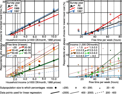
Systematic choice for the alternatives with the shortest available travel time yields 111 111 111 111 (see Table 1). This was exhibited by 656 respondents, making up an ample 9% of the combined 1988 and 1997 survey population. Systematic choice for the cheapest alternatives results in CS 222 222 212 222 or 222 222 222 222, exhibited by 133 and 16 respondents, respectively, who together made up 2% of the combined population. Figure 1 shows the recorded occurrence of these CSs as function of survey year, income and free time. Dots, indicating the percentages of lexicographic answerers for different income and free-time classes, are positioned at the class medians. The depicted trends are determined with simple linear regression, accounting for income and free-time class sizes. I found very similar trends when individual-specific free-time budgets were considered instead of class-medians.
The left-hand side of Figure 1 demonstrates that in all considered subpopulations the percentages of the respondents who systematically choose the alternative with the shortest travel time increased with household income. At the aggregated 1988 and 1997 levels, this trend predicts zero lexicographic choice. The higher frequency in 1997 compared to 1988 is consistent with the about 25% decrease in the real value of the cost-attribute level due to inflation: in 1997 10% lexicographic answering occurred at approximately 4,800 Dfl/month, in 1988 at approximately 6,400 Dfl/month. It nevertheless shows a clear decrease in frequency with decreasing income. Though some low-income respondents with very little free time choose for the shortest travel time, no one with ample time budget and low income did so. All systematic choice for the shortest travel time can thus be explained by trading respondents applying a WADD rule.
The right-side diagrams of Figure 1 are similar to those at the left side, though the percentages are much lower. The noisy character of this diagram goes together with small subpopulation sizes. In all considered subpopulations the percentage of the respondents who systematically choose the alternative with the lowest cost increased with increasing free time. The lower frequency in 1997 compared to 1988 is consistent with the decrease in the real value of the cost-attribute levels. Extrapolation to a zero-free-time budget again predicts zero lexicographic choice, except for the respondents in the lowest income class. Lexicographic answering for the lowest travel cost can thus also be explained by respondents applying a WADD rule.
A few respondents (0.17% of the survey population) systematically selected the alternatives with the highest cost. This might possibly be caused by an indiscriminately adopted lexicographic rule.
People with a strong status-quo preference with respect to travel time may always select the alternative with the smallest feasible travel-time change. Just one respondent completed a CS that might have followed from such a rule. Two other respondents systematically selected all alternatives with zero time change. Such weak-lexicographic algorithms may be adopted because of narrow departure-time and arrival-time constraints, for example. Another explanation might be people whose ideal travel time is equal to that experienced during the recruitment trip. But random choice, for example, could yield the same CSs.
The relative position of the alternatives in choice sets yields an inevitable additional attribute in any stated-choice questionnaire. This offers the opportunity to simplify the choice task by selecting the left- side or right-side alternative. Hess, Rose & Polak (2010), for example, found that 1.1% of the respondents in the Danish VTTS survey followed one of these strategies. In the Dutch surveys nobody completed one of the concerned CSs. Neither were any CSs recorded following from lexicographic algorithms like: six times left-right, three times twice left-twice right, two times thrice left-thrice right, six left-six right, four left-four right-four left, or four left-two right-two left-four right, and any of their right-left counterparts.
The comparisons of expected and recorded CS frequencies leave no reason to assume that a significant part of the survey population applied any of the non-trading lexicographic algorithms discussed above. Adding such an algorithm to a choice model with WADD algorithms will thus bias rather than improve its predictive usefulness, as it will inevitably over-predict strong-lexicographic answering among travellers with low income and ample free time.
This section presents a further elaboration of outcome-oriented inferential statistics, for the analysis of stated choice surveys in which the scale extension of attributes varies. A stochastic distribution of threshold levels over the population — a normal distribution, for example — is commonly assumed for elicitation of such algorithms (e.g., Cantillo & Ortúzar, 2005). I adopt this assumption here. It implies that differences in the ranges of attribute levels that are submitted in different stated-choice games will influence the occurrence-frequency of the CSs that are generated by the concerned algorithm. This allows estimating the frequency of occurrence of threshold-based algorithms. The only restriction is that the threshold-level-frequency distributions should be the same for all considered scale extensions. This approach is tested by exploring the contribution of 16 different algorithms to the explanation of the Dutch survey results. All are shown to have little if any relevance.
In Decision Theory several choice algorithms were defined that assume the elimination or selection of those alternatives that (dis)satisfy some threshold level on one or more attributes (e.g., Dawes, 1964; Tversky, 1972). Such algorithms draw on the assumption that those who employ them aim to reduce the complexity of their choice task. The algorithms may be considered on their own or in connection with a second-stage evaluation that can, for example, be compensatory or lexicographic (e.g., Gilbride & Allenby, 2004). Most algorithms imply elimination of alternatives with an unacceptably low attribute level. Others result in the selection of any alternative with an above-threshold level of a positively valued attribute. If an individual applies such an algorithm consistently as a first-stage rule, the number of feasible CSs that she can generate is restricted. For example, the SC sets of the Dutch surveys (see Table 1) imply that elimination of all alternatives with a time-increase threshold at zero minutes will result in one of the 16 possible CSs of type (a)6: 11x x11 x1x 111, in which x may depend on any second-stage evaluation. Likewise, a zero-Dfl cost-increase threshold yields one of the 32 CSs of type (c): xx2 22x xx2 222. Note that eight of the 16 different CSs that constitute (a) and another eight out of the 32 of (c) can just as well follow from WADD-LF (see Section 4). Among these are the lexicographic 111 111 111 111 and 222 222 2x2 222 that were discussed in the previous section.
In the Dutch surveys different stated-choice games were submitted to four subpopulations with different recruitment-trip-travel times (rtt). The games differed in the absolute scale extensions (ase) of the attributes. The maximum travel-time decreases and increases ranged from 10 min for respondents with rtt ≤ 45 min through 20 min (45 < rtt ≤ 90) and 30 min (90 < rtt ≤ 135) to 40 min (rtt > 135). The corresponding maximum cost increases ranged from Dfl 3 through Dfl 6 and Dfl 9 to Dfl 12 (see Table 1). The recorded CSs can thus be classified in the ase-classes 1 … 4 in which all attribute levels of the evaluated alternatives are proportionate to the class numbers. Respondents with a time-increase threshold between 0 and 5 min will then select (a): 11x x11 x1x 111 from games with ase = 1, 2, 3 and 4; a threshold between 5 and 10 min will yield (a) if ase = 2, 3 or 4 but not necessarily if ase = 1; thresholds between 10 and 15 min result in (a) if ase = 3 or 4; and thresholds between 15 and 20 min yield (a) if ase = 4. Members with a time-increase threshold between 5 and 10 min will select alt. 1 from SC 1, 5, 8 and 11 (see Table 1) and thus generate a CS belonging to the less restricted (b):7 1xx x1x x1x x1x if ase = 1. A time-increase threshold between 10 and 15 minutes will not manifest itself when ase = 1, yield (b) for ase = 2 and (a) for ase ≥ 3; thresholds between 15 and 20 min do not influence choice when ase = 1, yield (b) for ase = 2 and 3 and (a) for ase = 4; and thresholds between 20 and 40 min will not manifest themselves for ase = 1 and 2 but yield (b) for ase = 3 and 4.
Figure 2: Hypothetical time-threshold frequency distributions and their effect on CS occurrence.
Now imagine a subpopulation of respondents who actually eliminated all alternatives with an above-threshold time increase, followed by any second-stage evaluation of the remaining choice sets. It has some unknown frequency distribution of respondent-specific thresholds, which is considered to be the same for each ase class. Five hypothetical distributions are depicted on the left-hand side of Figure 2, exhibiting one, two or no peaks in the frequency of threshold occurrence. Following the reasoning in the previous paragraph the right-hand side in Figure 2 illustrates the strong effect that the unknown threshold-frequency distribution has on CS-type frequency. It also illustrates that the frequencies of (b) for ase = 1 and 2 are equal to those of (a) for ase = 2 and 4, successively. And the size of the subpopulation that exhibited elimination of alternatives with an above-threshold time increase follows from applying the type-(b) percentages for ase = 1, 2, 3 and 4 to the number of respondents who completed the corresponding stated-choice games.
Similarly, one can assume an imaginary subpopulation whose members eliminate all alternatives with an above-threshold cost increase, followed by any second-stage evaluation. Again, some unknown threshold-frequency distribution is supposed, now of cost-increase thresholds between zero and 12 Dfl. Because six different cost-increase levels were discerned in all ase classes, this algorithm can generate six different types of CSs, from the most restricted (c): xx222x xx2 222 for low thresholds trough (d): xx2 2xx xx2 222, (e): xx2 2xx xxx 2x2, (f): xxx 2xx xxx 2x2 and (g): xxx xxx xxx 2x2 till the least restricted (h): xxx xxx xxx xx2 for very high thresholds. CSs belonging to type (c) are a subset of all those belonging to types (d) through (h); (d) is a subset of (e) through (h), etc. Again, the frequency at lower ase levels of several less-restricted CS-types is the same as for more restricted types at higher levels. Some examples: CS-type (d) for ase = 1 and (c) for ase = 4; (g) for ase = 1 and (d) for ase = 2; and (g) for ase = 3 and (f) for ase = 4.
For these and other hypothetical subpopulations, whose members all employ the same absolute-attribute-threshold-based-elimination or selection algorithm, the following generalized relationships between CS-type frequency and ase appear to hold for any distribution of thresholds over the subpopulation:
Figure 3: “Upper-limit” assessment of the size of subpopulation A.
The frequencies of occurrence of relevant CS-types in each of the considered ase classes can be used to estimate the contribution of attribute-threshold-based algorithms to the explanation and prediction of choice behaviour. This can be done by conceiving the occurrence of CS-types as the outcome of choices by two subpopulations, subpopulation A whose members all generated CSs that will follow from application of that algorithm and B with people who generated CSs that will not.
Figure 3 illustrates how an “upper-limit” estimate can be assessed of the size of subpopulation A. The left-side and right-side diagrams do so for two different imaginary frequency-of-occurrence distributions of (a) and (b) over the survey population. Starting from the most restricted CS-type (a), the “upper-limit” for ase = 1 and 2 can be assessed from the occurrence of (a) for ase = 2 and 4, respectively (step 1 and 2). Next, the increase for ase = 3 and 4 compared to ase = 2 can be assessed from the corresponding increase in (b) (left-side diagram: step 3 followed by 4; right-side diagram: step 3 followed by 4 and 5).
The average upper-limit percentages, weighted for the shares of the population that completed the concerned ase-games, yields the share of subpopulation A within the survey population. In case of an equal distribution of the population over ase-classes this amounts to 27% and 19% for the left-side and right-side diagram in Figure 3, respectively. This would be a realistic estimate of the occurrence of the attribute-threshold-based algorithm if all concerned CSs were exclusively generated by this rule. But other algorithms might yield these same CSs. As elaborated in the previous subsection, the occurrence of this algorithm will not manifest itself if ase approaches zero. I used linear regression for estimating this zero-ase occurrence. A realistic estimate of the occurrence of the time-threshold-elimination algorithm can now be found by subtracting this zero-ase occurrence from the weighted-average size of subpopulation A. This yields 25% for the diagram on the left in Figure 3 and 6% for that on the right.
The assessment process as developed above can also be used to estimate the occurrence of other elimination and selection rules in the Dutch surveys. In the following paragraphs this will be done for two subpopulations, one whose members completed one of the 29 CSs that can follow from WADD-LF and a “rest-subpopulation” for whose recorded CSs this does not hold. For different threshold-based elimination and selection algorithms I assess the CS-types that these will generate. For both subpopulations I test with simple linear regression whether the relevant CS-type frequencies decreased with ase. If so, I considered that the algorithm that brought these about was irrelevant for the explanation of the recorded choice behaviour. If not, I estimated the realistic frequencies of occurrence of the concerned algorithm.
Figure 4: Conjunctive elimination of alternatives with above-threshold time and cost increases.
The conjunctive choice rule (Dawes, 1964) presumes that an individual rejects all alternatives that do not meet a minimum level on each attribute. It reduces to elimination of alternatives with an above-time-increase threshold if the cost-increase threshold is not considered and/or higher than the highest considered cost increase. The types (a) and (b) that this latter algorithm generate were discussed extensively above. The left-hand side of Figure 4 depicts their frequencies of occurrence in the Dutch surveys. It shows that about two-thirds of all individuals may have applied it as a first-stage rule. For the vast majority of these, WADD-LF offers an overlapping explanation. The regression lines exhibit a frequency-increase of (a) and (b) with ase. The “realistic estimate” assessment yields that the absolute-above-threshold-time-increase elimination may explain the choices of 2.1% of the survey population of which less than 0.7% cannot be explained from application of WADD-LF.
If the time-increase threshold is not considered and/or higher than the highest considered time increase, the conjunctive rule reduces to elimination of alternatives with an above-cost-increase threshold. The CS-types (c) up to and including (h) that this algorithm generates were elaborated above. The middle diagram of Figure 4 shows their frequencies of occurrence.8 It appears that 87% of all individuals may have applied it as a first-stage rule. The slopes of the regression lines are clearly negative for (c) through (h). Absolute-above-threshold-cost-increase-elimination algorithms are thus irrelevant for the explanation of the Dutch survey results.
The “general” conjunctive choice rule rejects all alternatives that do not meet a minimum threshold on each attribute. A time-increase threshold can be effective for SC 1, 2, 6 and 8 and a cost-increase threshold for SC 3, 4 and 9. For the SC-sets 5, 10, 11 and 12 both a cost- and time-increase threshold can be effective (see Table 1). After a second-stage evaluation and/or if the cost-increase or time-increase threshold becomes sufficiently high these latter can thus yield either alt. 1 or alt. 2. Following the same reasoning as for the elimination algorithms above, the general conjunctive algorithm might yield (i): 112 211 x12 xxx through (r): 1xx x1x x1x x12. These frequencies of occurrence are depicted in the right-hand side of Figure 4. They show a decline or negligible increase with ase, except for (r), (k) and (l) – both latter as far as WADD-LF offers an alternative explanation. The realistic-estimate-assessment yielded zero general-conjunctive-rule-applying respondents.
Apparently, the three conjunctive algorithms with an absolute threshold specification together may explain about 2% of the survey results, of which about one-third does not follow from WADD-LF. For about half of these latter, other compensatory rules offered alternative explanations. Altogether I conclude that these algorithms do not contribute to the explanation of the Dutch surveys.
The disjunctive choice rule results in “the acceptance of any alternative with an attribute that exceeds a certain criterion” (Foerster, 1979, p. 21, referring to Dawes, 1964). It may be followed by any second-stage evaluation of the remaining unsettled choice sets. If the cost-decrease threshold is not considered, such respondents will select any alternative with an above-threshold time decrease. This is applicable to all choice sets except SC 1, 2, 11 and 12, in which no alternatives with time decrease are available. A subpopulation applying this disjunctive algorithm may generate (s): xx1 111 111 1xx and the less constraint (t): xxx 111 xxx 1xx. Following the same procedure CS-types (u) through (x) are found for a subpopulation that selects any alternative with an above-threshold cost decrease, and (y) through (ae) if both a time- and cost-increase threshold are applied.
Similar to those for the conjunctive algorithms I established the frequencies of occurrence and linear regression lines of (s) and (t). Almost 20% of the survey population generated (t) and could have applied this disjunctive algorithm in a two-stage choice process. The frequencies of both (s) and (t) increase with ase. A realistic estimate of 1.6% was found, completely restricted to the rest-subpopulation. It appears that by far most CSs classified in (t) are also part of (b) and thus may be explained by application of conjunctive elimination of alternatives with above-threshold time increases.
In addition to conjunctive elimination of alternatives with above-threshold time increases, disjunctive selection for alternatives with above-threshold time decreases may thus explain less than 1% of the survey results. Analysis of the frequencies of (u) through (x) yields that 0.9% of all respondents may have exhibited a disjunctive preference for travel tame savings. Of these, 9 in 10 may have applied WADD-LF instead. Disjunctive choice in which both cost- and time-decrease thresholds were applied could explain the choices of far less than 0.1%. The contribution that disjunctive selection algorithms may offer to the explanation of the Dutch survey is thus a modest to marginal 1% at most.
Figure 5: Elimination-by-Aspects.
Elimination-by-Aspects as posited by Tversky (1972) assumes that the chooser has a threshold level for all attributes but follows a stochastic order of attribute evaluation, which order may vary during the completion of a choice sequence. If an alternative does not meet the threshold criterion of the first considered attribute, it is rejected and the alternative that remains is chosen; if more alternatives remain, another attribute is considered in the same way, until one alternative remains. For a subpopulation employing this algorithm I assumed a similar distribution of threshold levels over the survey population as for the general conjunctive algorithm.
The stochastic character of this algorithm means that its application by an individual can result in any feasible CS. However, if a subpopulation that applies it consistently is sufficiently large, the frequency of alt. 1 choices from all SC sets 1, 2, 6 and 8 as well as the frequency of alt. 2 choices from all SC sets 3, 4 and 9 should increase with scale extension. Following the CS-type notation adopted above this should hold for all CS-types (A): 1xx xxx xxx xxx up to and including (G): xxx xxx xx2 xxx. Figure 5 shows the actual trends for the rest-subpopulation. Those for the subpopulation which may have applied WADD-LF exhibited the same patterns. The frequencies of some of these CS-types increase with scale while others decrease. It shows that Elimination-by-Aspects does not contribute to the explanation of the Dutch survey results.
By analogy I considered Selection-by-Aspects: following a stochastic order of attribute evaluation, which order may vary during the completion of the choice task, alternatives with above-threshold time or cost decreases are accepted. If a subpopulation would apply this algorithm consistently, the frequency of the relevant CS-types (H) through (M) should also increase with scale extension. But the frequencies of some of these increase with ase while those of others decrease. Apparently Selection-by-Aspects does not contribute to the explanation of the Dutch survey results.
From a behavioural point of view, choice algorithms considering thresholds as fraction of recently experienced attribute levels might be more plausible than those based on absolute levels. For the Dutch respondents, the actual travel time (ta) during their recruitment trip may have been the experience that first came to their mind, as they had to report it extensively just before completing the stated-choice game. That is why I also considered relative thresholds in terms of the ratios of absolute time-attribute levels and the actually experienced recruitment-trip duration. The corresponding relative-time-change scale extensions (rse) are 10/ta, 20/ta, 30/ta or 40/ta, depending on the ase of the completed stated-choice game. As ta and ase vary from one respondent to the other this holds for rse, too. I attributed all respondents to four time-rse classes: <25%; 25 to 30%; 30 to 35%; and >35%. The Dutch surveys did not ask for the respondents’ recruitment trip expenses (ca). I considered these as approximatively proportionate to travel time, thus ca = α · ta. Under this assumption the time-change-rse percentages can be used to delimit the same rse classes as corresponding cost-change-rse percentages would do.
I tested the eight choice algorithms that were considered above with an absolute threshold-level specification, now using relative-threshold specifications. Elimination-by-Aspects and Selection-by-Aspects showed the same patterns: the frequencies of some of the relevant CS-types increase with scale extension while others decrease. Disjunctive selection, in its general version and with time-decrease thresholds only, did not explain any choice record. Conjunctive elimination with a relative time-increase threshold (0.2%) and in its general guise (0.7%, for two-thirds overlapping with WADD-LF) also appeared irrelevant. Conjunctive elimination of alternatives with an above-relative-threshold-cost increase could explain 3.8% of all responses, for most part overlapping with WADD-LF. Disjunctive selection of alternatives with above-relative-threshold-cost-decreases could explain 2.7% but this overlapped completely with the corresponding conjunctive rule and with WADD-LF. Taking the overlapping explanations into account yield that about 4% of all responses may be explained by conjunctive elimination algorithms with relative threshold specifications, for 3% of which WADD-LF offers an alternative explanation.
All respondents to the Dutch surveys, except for 10 of them who violated dominance, generated CSs that would result from application as a first-stage rule of one of the 16 attribute-threshold-based choice algorithms discussed above. But none of these rules could settle all 12 choice decisions. A second-stage evaluation is needed to decide about four to 11 choice sets. For most recorded CSs compensatory algorithms offer an alternative explanation; for 78% of all respondents (see Section 4) these algorithms are also the obvious second-stage-evaluation rules. This leaves 22% of all respondents who may have used alternative algorithms as such. For one-third of them (7%), this may have been a second-stage random rule (see Appendix 2 for the frequency-assessment procedure). Another one-third of them violated dominance and thus apparently used some obscure algorithm, either as a second-stage rule or, more obvious, instead of a two-stage attribute-threshold-based algorithm. Finally, about one-third of them (8%) may have applied WADD-LF as a second-stage rule. This is far more than the share of the survey population that, according to the previous paragraphs, may actually have used any first-stage elimination or selection rule. “Missing” explanations for second-stage choice decisions are thus no reason to reduce this latter share.
By far most CSs that were recorded in the Dutch surveys could have resulted from more than one first-stage attribute-threshold-based elimination or selection algorithm. If so, the second-stage evaluation could have been WADD-LF in the majority of cases. The latter algorithm applied on its own could explain most of these CSs. For their occurrence are thus most often several overlapping explanations.
The analyses above showed that the 16 considered elimination and selection algorithms together can explain about 8% of the outcomes of the Dutch surveys, almost equally distributed over algorithms with absolute and relative threshold specifications. Most plausible appeared the conjunctive algorithms with an absolute-time-increase threshold (2.1%) and with a relative-cost-increase threshold (3.8%). WADD-LF can account for the second-stage evaluations of by far most of these non-compensatory rules. But for about two-thirds of them a more frugal explanation is a one-stage WADD-LF assessment. This leaves about 3% remaining CSs for which one of these first-stage elimination and/or selection rules offers an explanation that does not overlap with WADD-LF. But one-stage random choice, other compensatory rules, obscure algorithms resulting in dominance violations and mistakes that are not considered here may offer other explanations for most of these. Their contribution to the explanation of the Dutch surveys is thus marginal at most.
The aim of this study is to explore the extent to which different choice algorithms can explain the choice data acquired in large-scale choice surveys. In applied sciences such surveys are a popular means to acquire insights in the choices that people make in everyday life. The explanatory algorithms uncovered from such studies are useful building blocks for models meant for the prediction of behaviour in contexts that differ from the estimation context. But the latter requires tailor-made transferability to the prediction context. If different choice algorithms co-occur within the survey population, understanding their distribution is very important because different algorithms can imply different transferability relations.
Random Utility Maximization (RUM) is the de facto standard in many analyses of choice data. With very few exceptions the common version of the WADD rule is assumed for the assessment of the alternatives’ utilities (McFadden, 2001). Analyses that pre-assume this rule for each respondent do not allow inferences about the occurrence of other choice algorithms that consumers may have used actually. As the respondents’ choice set compositions, including attribute levels, as well as their decisions are recorded in the large-scale choice surveys of applied sciences, the outcome-oriented approach from psychological research of judgment and decision-making seems the obvious way for the current research. But this approach commonly reveals different algorithms that explain the same choice behaviour.
The outcome-oriented inferential statistics approach was proposed in Section 2 to reduce this overlap. It focuses on the analysis of the individuals’ choice patterns (termed CSs here) rather than their separate choices. It considers the causal relationships between an individual’s personal circumstances, his use of a particular algorithm and the resulting choice pattern and employs inferential statistics for analysing the frequencies of the expected and actually recorded CSs within groups of respondents. In Appendix 1 it is tested for fictitious stated choice surveys with small and large survey populations. It appeared feasible to assess frequency distributions of the partly overlapping occurrence of three considered explanatory algorithms over the survey populations. It showed a clear decline of the elicited overlap with increasing survey population size; for a small population, too, a distribution could be assessed, although with larger bandwidths of overlapping explanations.
This method was applied for eliciting different non-compensatory algorithms from Dutch survey results. It allowed disentangling, at the aggregate level, the overlap in explaining compensatory and non-compensatory algorithms to a large extent. I consider this discriminatory power of outcome-oriented inferential statistics the most promising finding from the present study and recommend testing of this approach to the outcomes of other surveys, to see whether or not its performance survives. Other potential applications of the method are: investigating the relevance of different kinds of human errors, and discriminating between different WADD-algorithms.
In applied sciences it is often assumed that all respondents employ the WADD-algorithm, while since Simon (1955) the use of non-compensatory instead of compensatory choice algorithms has been a major research topic in psychological research of human judgment and decision-making. That is why I examined whether or not non-compensatory algorithms, if added to a mixture of compensatory algorithms, may explain the choice behaviour of a larger share of the survey population. First, algorithms complying with WADD (Payne et al., 1993) were considered (Section 4). If faultlessly and deterministically applied in its most constraint interpretation – linear-additive utility of attribute levels, but taking all feasible attribute weights/VTTS-values into consideration – it could explain the choice behaviour of 31% of the survey population. WADD-LF, with loss aversion factors between 1.0 and 2.5, explained these same and another 37%. Higher loss aversion factors, allowing for diminishing marginal utility (concave value function) and/or diminishing sensitivity (convex in loss domain, concave for gains) raised the percentage of the survey population that may have used a compensatory WADD-rule to 78%. This leaves 22% of the respondents who did not apply one of these WADD rules faultlessly.
Concerning non-compensatory rules, by definition Random choice could result in any CS generated by a particular respondent, if viewed apart. Lexicographic choice for the cheapest or shortest trip would result in one out of three different CSs that were recorded for 11% of the survey population and one or more of 16 different attribute-threshold-based elimination and selection algorithms could, applied as a first-stage rule, explain the CSs of 99.9% in part. If combined with a secondary-stage compensatory rule these latter could yield 85% of all responses, including all that would also follow from one-stage compensatory assessment. Second-stage random choice and unknown algorithms resulting in dominance violations each could explain half of the remaining 15%.
Analyses following outcome-oriented inferential statistics showed that, at the aggregate level, as many as 2% of all respondents may have exhibited random choice (Appendix 2). Except for 0.1% of the survey population, this offered no alternative explanation for the exhibits of WADD-LF. Such analyses also revealed a virtually zero occurrence of “true” lexicographic choice rules (Section 5) and showed that in just about 8% of all responses any of the 16 considered elimination and selection rules (Section 6) may have been applied as a first-stage evaluation. For two-thirds these latter could have been followed by a compensatory second-stage assessment. For parsimony reasons, assuming such a two-stage evaluation makes little sense, as a one-stage compensatory algorithm would yield the same result. That leaves about 3% of the survey population who may have applied one of the 16 considered elimination and selection rules as a first-stage choice rule. These 3% are distributed over algorithms with absolute and relative threshold specifications. This clearly contradicts my earlier suggestion that non-compensatory decision strategies can explain most CSs that could not follow from WADD-LF (Van de Kaa, 2006). From the current findings I conclude that faultless application of WADD in a broad sense can explain almost 80% of all responses, for which the considered random, lexicographic and attribute-threshold-based non-compensatory algorithms do not offer alternative explanations; and that mistakes, not-considered compensatory rules and unknown algorithms resulting in dominance violations may explain most of the remaining responses.
At first sight the limited explanatory performance of non-compensatory algorithms did not come as a surprise: the design of the Dutch surveys, with a limited number of two-alternatives-two-attributes choice sets and no time pressure, seemingly yielded a simple choice task. And several experiments showed that when the complexity of the choice task increases there is a shift from compensatory to non-compensatory decision rules — see Rieskamp and Hoffrage, 1999, for an overview. But a scan of the empirical evidence advanced in the studies that they cited revealed extensive use of non-compensatory rules in the choice tasks that were deemed relatively simple (e.g., Sundström, 1987; Payne, Bettman & Luce, 1996). Presumably the simplest choice task that I retrieved in this scan concerned choice, under no time pressure, from sets with two alternatives, each with three attributes, whose levels were indicated in the same dimension: a positively valued natural number from 1 to 5 - see e.g., Svenson, Edland and Slovic (1990) and Edland (1993). From these and two similar Swedish studies it appeared that non-compensatory algorithms could explain many or even most of the choices in this context. This is conspicuous as the setting allows compensatory choice assessment by just twice adding three natural numbers, followed by deciding which of both sums is highest; to me, this seems the cognitively least demanding compensatory algorithm imaginable. The Dutch surveys, too, have two alternatives in each choice set, and only two instead of three attributes. But these attributes are time and cost changes indicated by rational instead of natural numbers, not given in the same dimensions but in two different ones and such that the numerical values of the time-change-attribute levels (given in minutes) are almost an order-of-magnitude larger than those of the cost-changes (in Dfl) (see Table 1). Moreover, these levels are presented as positive numbers but from a cue (increase or decrease) embedded in a verbal description the respondents have to decide whether these should be considered as positive or negative. Application of the conventional WADD rule in the Dutch surveys will thus imply four sign attributions, cross-dimensional mappings/multiplications, additions, subtractions and comparisons of two not-shown natural numbers. This seems cognitively much more demanding to me than the task in the Swedish studies. And WADD-LF could explain much more responses by considering different loss-aversion factors, which latter will make the choice task increasingly complex. Even more complex is the application of non-linear attribute-value functions, which explains another 10% of all responses. Lexicographic choice for the alternative with the lowest travel time from the Dutch stated choice games requires just two sign attributions and comparison of two natural numbers that are explicitly shown in the questionnaire. From that point of view I consider the inferred explanatory performance of the WADD-algorithms in the Dutch survey context, at the expense of lexicographic choice or attribute-threshold-based rules, as far from self-evident.
Consistent, conscious application of the algorithms that yield the same choices as were observed would thus require cognitively quite demanding calculations. But this study only shows that, under similar personal circumstances, most respondents made exactly the same choices as many others did. From a functional perspective on human choice (Van de Kaa, 2008, 2010b) this implies that the rules and/or heuristics adopted by many different people arrange for the same transformation of submitted alternatives into choices. I consider it implausible that many respondents actually applied one of these WADD algorithms consciously, let alone that app. 80% did so. If I am right, this study suggests that in everyday choice people intuitively deploy heuristics that are fit to transform contextual information into choices that should serve their interests; that similar personal circumstances invoke heuristics from the adaptive toolboxes of many different people that provide similar transformations, resulting in the same decisions; that these heuristics may require much more cognitive effort than non-compensatory algorithms would do; and that the mind can easily exert this effort. In other words, I believe that most adaptive decision makers employ fast and functional heuristics that may be far from frugal; reducing cognitive effort does not seem to play an important role in their adoption.
I also found the strong degree to which people attach a higher weight to travel-time (or cost) savings when they have less free time (or earn less money) conspicuous (see e.g., Figure 1). It underlines the relevance of long-established psychological principles, like decreasing marginal utility (Bernoulli, 1738), for the understanding of contemporary everyday choices. Furthermore, the survey respondents covered the whole range of incomes, jobs, trip purposes, travel modes, household types etc. as were common in the Netherlands in 1988 and 1997. It struck me that 80% of this very heterogeneous population generated less than 1% of all feasible CSs that, in turn, almost all would follow from faultless application of just a few WADD-algorithms. Perhaps everyday human choice is more consistent and less stochastic and error-prone than some contemporary choice paradigms assume.
Returning from feeling to findings: taking things together the present study does not shed more light on the choice algorithm that any particular respondent actually employed. But at the aggregate-population level, it revealed that WADD-algorithms incorporating different degrees of loss aversion could explain, or rather simulate, by far most of the recorded choice behaviour while none of many non-compensatory algorithms that were considered yielded a more than marginal explanation. Replications of this study, preferably by re-analysing other large-scale surveys with more complicated choice sets, are recommended to find out whether or not these findings are incidental.
The present re-analyses of the Dutch national VTTS surveys show that choice data that were collected and filed in 1988 and 1997 are still useful for testing new research approaches and for improving our understanding of human choice behaviour. Thanks to this journal there is now open access to these data for other researchers. In travel behaviour research there are dozens of large-scale stated choice surveys that may still lay waste in archives, and it is hard to believe that the situation is different in other applied disciplines like marketing and environmental science, for example. Most of these studies were publicly funded, and this fact may lend support to requests for unlocking the data in an open-access website, like the World Database of Happiness (Veenhoven, 2014), for example. This opportunity could give a boost to psychological and interdisciplinary research of choice behaviour. It would be great if an international non-profit organization, maybe the Society for Judgment and Decision-Making, or one of its members would take the initiative to organise this.
Ballinger, T. P. & Wilcox, N. T. (1997). Decisions, error and heterogeneity. The Economic Journal, 107(443), 1090–1105.
Bernoulli, D. (1738). Exposition of a new theory on the measurement of risk (English translation from Latin, republished 1954). Econometrica, 22(1), 23–36.
Bröder, A. (2010). Outcome-based strategy classification. In A. Glöckner & C. L. M. Witteman (eds.), Foundations for tracing intuition: Challenges and methods, pp. 61–82. London: Psychology Press & Routledge.
Burge, P., Rohr, C., Vuk, G., & Bates, J. (2004) Review of international experience in VOT study design. European Transport Conference, Strasbourg.
Cantillo, V. & Ortúzar, J. d. D. (2005). A semi-compensatory discrete choice model with explicit attribute thresholds of perception. Transportation Research Part B, 39(7), 641–657.
Dawes, R. M. (1964). Social selection based on multidimensional criteria. Journal of Abnormal and Social Psychology, 68(1), 104–109.
DeSerpa, A. C. (1971). A theory of the economics of time. The Economic Journal, 81(324), 828–846.
Dieckmann, A., Dippold, K., & Dietrich, H. (2009). Compensatory versus noncompensatory models for predicting consumer preferences. Judgment and Decision Making, 4(3), 200–213.
Edland, A. (1993). The effects of time pressure on choices and judgments of candidates to a university program. In: O. Svenson & A. J. Maule (eds.), Time pressure and stress in human judgment and decision making, pp. 145–156. New York: Plenum Press.
Foerster, J. F. (1979). Mode choice decision process models: A comparison of compensatory and non-compensatory structures. Transportation Research Part A, 13(1), 17–28.
Friedman, M. (1953). The methodology of positive economics. In M. Friedman (ed.), Essays in positive economics, pp. 3–43. Chicago: University of Chicago Press.
Gilbride, T. J. & Allenby, G. M. (2004). A choice model with conjunctive, disjunctive, and compensatory screening rules. Marketing Science, 23(3), 391–406.
Glöckner, A. (2009). Investigating intuitive and deliberate processes statistically: The multiple-measure maximum likelihood strategy classification method. Judgment and Decision Making, 4(3), 186-199.
Glöckner, A., & Bröder, A. (2011). Processing of recognition information and additional cues: A model-based analysis of choice, confidence, and response time. Judgment and Decision Making, 6(1), 23–44.
Gunn, H. (2001). Spatial and temporal transferability of relationships between travel demand, trip cost and travel time. Transportation Research Part E, 37(2-3), 163–189.
HCG (1990). The Netherlands’ value of time study: Final report. The Hague: HCG.
HCG (1998). Value of Dutch travel time savings in 1997 — final report. The Hague: HCG.
Hess, S., Rose, J. M. & Polak, J. (2010). Non-trading, lexicographic and inconsistent behaviour in stated choice data. Transportation Research Part D, 15(7), 405–417.
Hilbig, B. E. (2014). On the role of recognition in consumer choice: A model comparison. Judgment and Decision Making, 9(1), 51–57.
Hoffman, P. J. (1960). The paramorphic representation of clinical judgment. Psychological Bulletin, 57(2), 116–131.
Jara-Díaz, S. R. & Guevara, C. A. (2003). Behind the subjective value of travel time savings. Journal of Transport Economics and Policy, 37(1), 29–46.
Johnson, E. J., Payne, J. W. & Bettman, J. R. (1993). Adapting to time constraints. In O. Svenson & A. J. Maule (eds.), Time pressure and stress in human judgment and decision making, pp. 103–116. New York: Plenum Press.
Kahneman, D. & Tversky, A. (1979). Prospect theory: An analysis of decision under risk. Econometrica, 47(2), 263–291.
Killi, M., Nossum, Å. & Veisten, K. (2007). Lexicographic answering in travel choice: Insufficient scale extensions and steep indifference curves? European Journal of Transport and Infrastructure Research, 7(1), 39–62.
Luce, R. D. (1956). Semiorders and a theory of utility discrimination. Econometrica, 24(2), 178–191.
McFadden, D. L. (2001). Economic choices (revised Nobel prize lecture). The American Economic Review, 91(3), 351–378.
Payne, J. W., Bettman, J. R. & Johnson, E. J. (1993). The adaptive decision maker. New York: Cambridge Univ. Press.
Payne, J. W., Bettman, J. R. & Luce, M. F. (1996). When time is money: Decision behavior under opportunity-cost time pressure. Organizational Behavior and Human Decision Processes, 66(2), 131–152.
Rieskamp, J. & Hoffrage, U. (1999). When do people use simple heuristics and how can we tell? In G. Gigerenzer, P. M. Todd & ABC Group (eds.) Simple heuristics that make us smart, pp. 141–167. Oxford, UK: Oxford University Press.
Rosenberger, R. S., Peterson, G. L., Clarke, A. & Brown, T. C. (2003). Measuring dispositions for lexicographic preferences of environmental goods: Integrating economics, psychology and ethics. Ecological Economics, 44(1), 63–76.
Simon, H. A. (1955). A behavioral model of rational choice. Quarterly Journal of Economics 69(1), 99–118.
Montgomery, H. & Svenson, O. (eds.) (1989). Process and structure in human decision making. Chichester: John Wiley and Sons.
Norman, D. A. (1981). Categorization of action slips. Psychological Review, 88(1), 1–15.
Ramos, G. M., Daamen, W., & Hoogendoorn, S. (2013). Modelling travellers’ heterogeneous route choice behaviour as prospect maximizers. Journal of Choice Modelling, 6, 17–33.
Reason, J. (1990). Human error. Cambridge, UK: Cambridge University Press.
Riedl, R., Brandstätter, E., & Roithmayr, F. (2008). Identifying decision strategies: A process-and outcome-based classification method. Behavior Research Methods, 40(3), 795–807.
Svenson, O., Edland, A. and Slovic, P. (1990). Choices and judgments of incompletely described decision alternatives under time pressure. Acta Psychologica, 75, 153–169.
Sundström, G. A. (1987). Information search and decision making: The effects of information displays. Acta Psychologica, 65(2), 165–179
Swait, J. (2001). A non-compensatory choice model incorporating attribute cutoffs. Transportation Research Part B, 35(10), 903–928
Thoma, V., & Williams, A. (2013). The devil you know: The effect of brand recognition and product ratings on consumer choice. Judgment and Decision Making, 8(1), 34–44.
Tversky, A. (1972). Elimination by aspects: A theory of choice. Psychological Review, 84(4), 327–352.
Tversky, A. & Kahneman, D. (1991). Loss aversion in riskless choice: A reference-dependent model. The Quarterly Journal of Economics, 106(4), 1039–1061.
Van de Kaa, E. J. (2006). Assessment of the value of travel time from stated choice surveys: The impact of lexicographic answering. European Transport Conference.
Van de Kaa, E. J. (2008). Extended Prospect Theory. Findings on choice behaviour from economics and the behavioural sciences and their relevance for travel behaviour. Delft: TRAIL RS.
Van de Kaa, E. J. (2010a). Applicability of an Extended Prospect Theory to travel behaviour research: a meta-analysis. Transport Reviews, 30(6), 771–804.
Van de Kaa, E. J. (2010b). Prospect Theory and choice behaviour strategies: Review and synthesis of concepts from social and transport sciences. European Journal of Transport and Infrastructure Research 10(4), 299–329.
Van de Kaa, E. J. (2010c). Sign-dependent value of time in stated preference: Judgment bias or exposure of genuine preference? European Journal of Transport and Infrastructure Research, 10(4), 347–367.
Van den Broek, A., Breedveld, K., de Haan, J., de Hart, J. & Huysmans, F. (2004). Trends in time. The use and organization of time in the Netherlands, 1975–2000. The Hague: Social and Cultural Planning Office.
Veenhoven, R. (2014). World Database of Happiness. In A. C. Michalos (Ed.), Encyclopedia of Quality of Life and Well-Being Research, pp. 7257–7260. Dordrecht: Springer.
This appendix analyses the occurrence of choice algorithms that explain assumed distributions of choice sequences (CSs) in fictitious surveys. All participants in each imaginary survey are assumed to have stated their choices from c = 5 choice sets with each a = 2 alternatives. Each respondent thus generated one out of ac = 25 = 32 different CSs. In each survey, one or more respondents are assumed to have systematically selected the left-side alternative, thus giving rise to choice sequence CS1. One or more other respondents supposedly selected the alternative with the cheapest available cost attribute systematically and so generated CS2. Finally, the frequencies of occurrence of the remaining 30 CSs (CS3 to CS32) are assumed to be of the same order-of-magnitude.
For explanation of these imaginary surveys, three choice algorithms are considered: an inertia-driven left-side-preference rule, a budget-constraint-driven lexicographic preference for the cheapest alternative, and an inertia-driven random rule (Johnson et al., 1993). I assumed that all respondents applied one of these algorithms consistently. This implies that three subpopulations can be defined, each with members following just one of these algorithms. The rationale behind the left-side preference rule implies that CS1 is selected by anyone who applies it consistently. The rationale behind the lexicographic algorithm implies that CS2 is selected by anyone who applies it consistently. The rationale behind the random rule is randomly selecting one of both alternatives from each choice set, irrespective of attribute levels, position on the questionnaire and personal circumstances. It implies equiprobable choice from available alternatives. As a consequence, the CSs generated by a subpopulation of n random choosers are stochastically independent and their probabilities follow a binomial distribution. Thus, in this context with c = 5 choice sets each containing a =2 different alternatives, each feasible choice sequence f (CS1 … CS32) can be generated by any random chooser with a probability of occurrence є = a−c = 3.1%; and the probability that a particular f is chosen of times by no more or less than k random choosers equals
| Pr(of = k) = |
| · єk · (1−є)n−k (4) |
For any given subpopulation of n random choosers, the probability that CS1, CS2 (and any CS3 … CS32) is generated more or less than k times can now be calculated straightforward.
The size of the random-choice subpopulation equals the total survey population minus the left-side and lexicographic-preference subpopulations. The size of the subpopulations exhibiting left-side or lexicographic preferences equals the numbers of respondents who generated CS1 and CS2 minus those who did so by exhibiting random choice. Following the principles of inferential statistics I formulated sets of null-hypotheses (H0) to assess the latter numbers. One H0-set implied that members of the random-choice subpopulation generated less than k times CS1 and and/or CS2. If the predicted probability p of H0 becomes lower than the significance level α – here I adopted 1% – the maximum sizes of the subpopulations of respondents with left-side and lexicographic preferences are found by subtracting the thus found (k − 1) from the total recorded CS1 and CS2 numbers. Similarly, I formulated a set of null-hypotheses that the members of the random-choice subpopulation generated more than k times CS1 and/or CS2. Again, the k-values for which the predicted probabilities drop just below 1% are subtracted from the total numbers of recorded CS1 and CS2, which yields the minimum subpopulation sizes of respondents with left-side and lexicographic preferences. The maximum and minimum random-choice-subpopulation sizes are found by subtracting, respectively, the minimum and maximum sizes of left-side-choice and lexicographic-choice subpopulations from the total survey population. The difference between maximum and minimum sizes of these latter subpopulations indicates the degree to which random choice offers an overlapping explanation for left-side preference and lexicographic choice. Clearly, assessing the different subpopulation sizes requires an iterative process. In the following examples I use the size of the whole survey population as a first iteration of the random-choice-subpopulation size.
Example 1: In a small survey CS1 and CS2 were generated by 5% of all 40 respondents. In this imaginary survey two respondents complied CS1 and another two CS2. The probability that n = 40 random choosers generate CS1 once or less appears to be p = 64%; the probability that they generate CS1 twice or more is 36%; and the same percentages hold for CS2. An iteration with n = 36 yields similarly high p-values. Thus, none of the considered H0-hypotheses is rejected and the minimum and maximum sizes of left-side-preference and lexicographic-choice subpopulations are 0% and 5%. It implies that between 90% and 100% of all respondents chose as if they applied the random rule while 0%–5% may have exhibited a left-side-preference and 0%–5% a lexicographic preference for the cheapest alternative. Adding the latter algorithms to a random-choice model does thus not offer a statistically significant contribution to the explanation of the choice behaviour in this fictitious survey.
Example 2: In a small survey CS1 was generated by 5% and CS2 by 75% of all 40 respondents. Thus, two respondents generated CS1 and 32 CS2. In a first iteration, with n = 40, none of the considered H0-hypotheses is rejected for CS1. But the probability that CS2 is generated more than 4 times is well below p = 1%. Thus, it is almost certain that at least 28 respondents did not apply the random rule for generating CS2. This puts the maximum number of random choosers at n = 12 for the second iteration. After two more iterations it appears that lexicographic choice explains 75%–80% of the responses and random choice 15%–25%. For 5% of the responses lexicographic choice offers an overlapping explanation for random choice, and for another 5% left-side-preference does so. Adding the latter algorithm to a mixture of random and lexicographic choice algorithms does not offer a statistically significant contribution to the explanation of the choice behaviour in this fictitious survey.
Example 3: In a large survey CS1 and CS2 both were generated by 5% of all 1000 respondents. In this fictitious survey CS1 and CS2 were generated 50 times. Setting n at 1000 yields p < 1% for the probabilities that application of the random rule generates CS1 and CS2 less than 19 times. It also yields p < 1% for the probabilities that this generates these CSs more than 45 times. At the concerned levels both H0-hypotheses are thus rejected, implying that both left-side and lexicographic preference offer a statistically significant contribution to the explanation of the choice behaviour in this survey. In the next iterations, n was reduced with the subpopulation sizes of the almost certainly left-side and lexicographic choosers as found in the previous iteration. After three iterations it appears that random choice explains 91.4%–96.6% of all responses while left-side-preference and lexicographic choice each do so for 1.7%–4.3%. Adding the latter algorithms to a random-choice model does thus offer a small but statistically significant contribution to the explanation of the choice behaviour in this fictitious survey. Explanatory algorithms overlap for 5.2% of all responses.
Example 4: In a large survey CS1 was generated by 5% and CS2 by 75% of all 1000 respondents. Here, CS1 was completed by 50 respondents and CS2 by 750. Starting with n = 1000 shows that the random rule can explain less than 46 recordings of CS2. After three iterations it appears that random choice explains 20.2%–22.8% of all responses, lexicographic choice for the least expensive alternative accounts for 73.6%–74.9% and left-side-preference for 3.6%–4.9%. The statistically significant contribution of the latter algorithm to the explanation of the survey outcomes is thus substantially higher than in example 3. Overlapping explanations remain for just 2.6% of all responses.
The probability that a particular CS is generated by no more or less than k random choosers is discussed in Appendix 1 (Eq. 6). Starting with n = 7147 random choosers and a significance level α = 1% converges within four iterations. It yields a maximum of n = 395. For each of the s = ac = 4096 different feasible CSs the null-hypotheses that more than one of these 395 random choosers generated it has to be rejected (p = 0.44%) but the null-hypothesis that it is not generated at all cannot be rejected (p = 90.8%). Note, however, that with s different CSs the expected number of k-times-occurring CSs becomes
| s · Pr(of = k) = s · |
| · єk · (1 − є)n−k (5) |
According to this, 395 random choosers may generate an expected number of 359 once-occurring, 17 twice-occurring and zero to one thrice-occurring CSs. Now consider that all 4096 CSs should have an equal probability of being selected by a random chooser. The expected frequency of random-choice- generated CSs among the subset of 154 more than twice occurring CSs should thus be the same as for the remaining 3942. Taking this into account yields, after three iterations, an expected 207 random choosers, which constitute 2.9% of the survey population. I also considered that the expected frequency of random-choice-induced CSs should be the same for CSs with and without violation of dominance. This yields an expected 155 (2.2%) random choosers. Finally, the percentage of choices for alt. 1 and alt. 2 from each of the 12 choice sets should be the same for subpopulations who selected a once-occurring, a twice-occurring and a more-than-twice occurring CS.. I found that about two-thirds of the once-occurring and one-third of the twice-occurring CSs may be the consequence of random choice which, again, yields 2.2% random choosers among the survey population.
All three approaches show that random choice may explain an ample 2% of the Dutch survey results. But failures to apply another compensatory or non-compensatory algorithm consistently, due to errors and/or taste variations (not investigated here), may explain at least a part of the same CSs. The contribution of random choice to the explanation of the Dutch survey results is thus marginal.
The marginal utility of a decrease in travel expenses can be equated with the marginal value of income, while that of a decrease in travel time is equal to the marginal utility of substituting travel time for another activity (e.g., DeSerpa, 1971; Jara-Díaz & Guevara, 2003). In the context of the Dutch VTTS surveys, the participants’ working hours and other obligatory and personal time spending may be treated as constant – they are not exchangeable with travel time. This implies that an individual’s marginal utility of travel time can be equated to that of her free-time budget. Following Bernoulli (1738) an individual’s utility of a decrease in travel time will decrease in accordance with increases in his free-time budget; his utility of a decrease in travel expenses will decrease as his income increases. People who trade-off the utilities of time and money will thus systematically choose the alternative with the shortest travel time if their income is more than enough and/or their free-time budget is very limited. Likewise, the probability that such “trading” people systematically choose the alternative with the lowest expenses will decrease with income and increase with free-time budget. At the survey-population level, this means that the percentage of “traders” among the respondents who systematically choose the shortest feasible travel time approaches zero at zero income; and among the traders who prefer the cheapest trip alternative, that percentage approaches zero at a zero free-time budget. These features of utility theory also hold for the hedonic values of time and money gains according to Prospect Theory (Van de Kaa, 2010c).
The probability that a “non-trader” always chooses the alternatives with the highest time saving may increase with a decreasing free-time budget. However, by definition such a strong-lexicographic chooser should disregard cost levels. The probability should thus be the same for different incomes. Similarly, the probability that a non-trader always chooses the cheapest alternative may increase with decreasing income but should be the same for different free-time budgets. At the population level, this means that the percentage of non-traders among the respondents who systematically choose the shortest feasible travel time at zero income should also apply to other income levels. Likewise, the percentage of non-traders among those who systematically choose the cheapest alternative should be the same for all free-time levels.
I gratefully acknowledge Rijkswaterstaat for providing me with the Dutch VTTS survey results and for its consent to publish the Supplementary Data of this article, thus unlocking these for non-commercial use by other scientists provided that a proper reference is made. I thank Frank Hofman for his assistance in acquiring these permissions, and Jon Baron who challenged me to improve the receptivity of this article for the readers of Judgment and Decision making.
Copyright: © 2017. The authors license this article under the terms of the Creative Commons Attribution 3.0 License.
This document was translated from LATEX by HEVEA.