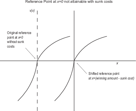
Figure 1: Incorporation of shifted reference point into prospect theory value function when sunk costs are present.
Option TK(D): P($0)=.90, P($45)=.07, P(−$10)=.01, P(−$15)=.02,
Judgment and Decision Making, Vol. 13, No. 6, November 2018, pp. 575-586
Why choose wisely if you have already paid? Sunk costs elicit stochastic dominance violationsRyan K. Jessup* Lily B. Assaad# Katherine Wick$ |
Sunk costs have been known to elicit violations of expected utility theory, in particular, the independence or cancellation axiom. Separately, violations of the stochastic dominance principle have been demonstrated in various settings despite the fact that descriptive models of choice favored in economics deem such violations irrational. However, it is currently unknown whether sunk costs also yield stochastic dominance violations. In two studies using a tri-colored roulette wheel choice task with non-equiprobable events yet equal payoffs, we observed that those who had sunk costs selected a stochastically dominated option significantly more than did those who had no costs. Moreover, a second study revealed that people chose a stochastically dominated option significantly more when the expected value was low compared to high. A model comparison of psychological explanations demonstrated that theories that incorporate a reference shift of the status quo could predict these sunk cost-based violations of stochastic dominance whereas other models could not.
Keywords: choice, decision, sunk cost, stochastic dominance, investment,
status quo effect, prospect theory, risk, model fitting, behavioral
economics, reference shift
In 2012 while working for JP Morgan, Bruno Iksil – otherwise known as the “London Whale” – gained notoriety when he was blamed for the loss of billions of dollars on credit default swaps. Through investigating the timeline of these losses, investigators discovered that when his initial investment decisions landed him substantially in the red, Iksil took major risks to double down on the losses rather than walk away. Instead of ignoring the sunk cost, Iksil scaled up the risk of his financial investments in order to try to recover from the initial losses (Hurtado, 2016).
Sunk costs refer to situations in which costs are irrevocably incurred regardless which future action is selected and, because all actions are equally affected, they should have no effect on decisions. However, the previous example demonstrates the power that sunk costs wield over decisions. The sunk cost fallacy occurs when the presence of sunk costs results in the choosing of different actions compared to when sunk costs are not present, thus violating the cancellation or independence axiom of expected utility theory (Machina, 1989).
In one of the most famous experimental studies on the sunk cost fallacy (Arkes & Blumer, 1985), two groups of subjects were asked to imagine that they were president of an airline company and then determine whether they would spend the last $1 million of their research funds to develop a plane that is undetectable by conventional radar. They are further informed that a competitor has just begun selling a similar plane that is both faster and more economical than the plane their company can build. Critically, the first group of subjects were informed that their firm had already spent $9 million on the project but the second group was not. 85% of the 48 subjects in the first group elected to continue with the project whereas only 17% of the 60 subjects in the second group chose to spend the funds, implicating the sunk costs in causing the differential choice behavior. Sunk cost effects have been found using a variety of experiments over multiple distinct domains and populations, suggesting that this is a reasonably well-supported effect in the literature (Navarro & Fantino, 2005; Strough, Mehta, McFall & Schuller, 2015; Tan & Yates, 1995; Zeng, Zhang, Chen, Yu & Gong, 2013).
Another element of rationality concerns the principle of stochastic dominance. This principle asserts that no rational individual or organization should ever choose a stochastically dominated option. Essentially, if option D never pays less and sometimes pays more than option W, then we say that option D stochastically dominates the weaker option W.1 Rank dependent models of choice (Quiggin, 1982), which are important for predicting economic behavior, retain this principle, despite the fact that violations of stochastic dominance have been observed in a variety of studies. This is not merely an ivory tower problem because, in its most simplified form, a violation of dominance reduces to a situation where an organization or individual prefers $8 over $10, all else being equal. The correct choice here is obvious. However, with increasing complexity it becomes less clear, even though the correct choice becomes no less dominant. Thus, violations of stochastic dominance are usually observed in nontransparent situations or involve between-subject designs (Birnbaum & Navarrete, 1998; Diederich & Busemeyer, 1999; Tversky & Kahneman, 1986).
When Kahneman and Tversky (1979) introduced prospect theory, mainstream economists eschewed it because it allowed for violations of stochastic dominance. Though they were aware of violations of stochastic dominance (Tversky & Kahneman, 1986), they nonetheless released a revised version of their model known as cumulative prospect theory (Tversky & Kahneman, 1992) that no longer allowed for violations of stochastic dominance.
However, violations of stochastic dominance continue to emerge. That violations of stochastic dominance occur in nontransparent designs is rather well-established. For example, Tversky & Kahneman (1986) demonstrated that when presented with the following pair of gambles,
Option TK(A): P($0)=.90, P($45)=.06, P($30)=.01, P(−$15)=.01, P(−$15)=.02Option TK(B): P($0)=.90, P($45)=.06, P($45)=.01, P(−$10)=.01, P(−$15)=.02,
individuals overwhelmingly prefer the dominant option TK(B). However, when the dominance of TK(B) is disguised using a nontransparent design, such as,
Option TK(C): P($0)=.90, P($45)=.06, P($30)=.01, P(−$15)=.03
Figure 1: Incorporation of shifted reference point into prospect theory value function when sunk costs are present. Option TK(D): P($0)=.90, P($45)=.07, P(−$10)=.01, P(−$15)=.02,
most subjects choose the weaker option, TK(C). The subadditivity principle of the probability weighting function of prospect theory (Kahneman & Tversky, 1979) allows it to account for these findings, but only when using separable decision weights, as opposed to the cumulative decision weights found in cumulative prospect theory (Tversky & Kahneman, 1992). Another example violation of stochastic dominance involving disguised dominance is demonstrated by Birnbaum and Navarette (1998) wherein they elicited preferences for the following two gambles:
Option BN(G+): P($12)=.05, P($14)=.05, P($96)=.90Option BN(G-): P($12)=.1, P($90)=.05, P($96)=.85.
They observed that 73/100 subjects preferred BN(G-) over BN(G+) despite the fact that G+ stochastically dominates, a result predicted by configural weight theory (Birnbaum & McIntosh, 1996). This is particularly interesting because configural weight theory also uses rank-dependent weights (like those used in cumulative prospect theory) on the outcomes but in a different way than more traditional versions (Quiggin, 1982; Tversky & Kahneman, 1992). Michael Birnbaum and his lab have replicated such effects many times (e.g., Birnbaum & Chavez, 1997; Birnbaum & Navarrete, 1998; Birnbaum, Patton & Lott, 1999).
Choice violations of stochastic dominance in transparent designs are much rarer and usually have very small effect sizes. For example, Diederich and Busemeyer (1999) presented evidence that subjects were significantly more likely to choose a stochastically dominated option when the outcomes were negatively correlated with those of the dominant option compared to when they were positively correlated.2 However, the overall probability of choosing the weaker option was rather low (e.g., in the between-subjects design, the more frequently chosen weaker option was only chosen 10% of the time). The multi-attribute implementation of decision field theory (Busemeyer & Townsend, 1993; Diederich & Busemeyer, 1999) was used to model the results, as the dynamic nature of the diffusion model – particularly, the attention switching component coupled with competitive evidence accumulation – yields increased selection of the weaker option when payoffs are negatively correlated.
Thus far, two primary ingredients in eliciting selection of a Stochastically dominated option have been found: (1) disguised dominance and (2) negatively correlated payoffs. But do other factors affect an individual’s propensity to select a stochastically dominated option?3 One intriguing possibility is the presence of sunk costs.
When subjects must financially invest before playing, their choices are taking place in a state of loss where theoretical and empirical work suggest they might be more prone toward risk-seeking behavior (Abdellaoui, Bleichrodt & l’Haridon, 2008; De Martino, Kumaran, Seymour & Dolan, 2006; Levy & Levy, 2002). Central to prospect theory is the idea that people derive value from gains and losses measured relative to a reference point. If no costs are present then individuals view any positive earnings as a gain and any negative earnings as losses with a reference point at zero. However, when pre-existing costs are present (i.e., sunk costs), individuals may no longer view a zero payoff as their reference point since it is no longer a possibility. For example, any gamble that requires a priori payment (hence, a sunk cost) will result in a positive outcome only with a win. All other outcomes are losses, and thus, a zero payoff is not attainable. The sunk cost shifts the reference point such that individuals are more willing to take risks to avoid the loss of not winning. Sunk costs may cause the target reference point to become the successful outcome (Figure 1). Due to the convexity of the curves in the loss domain, the prospects of the weaker option move nearer in value to the prospect of the dominant option. Thus, we would expect to see the frequency of stochastically dominated choices increase when sunk costs are present relative to when no costs are present.
First, our primary purpose was to test whether or not sunk costs increase the likelihood of making stochastic dominance violations. Second, we then want to see whether models which incorporate a shifted reference point are better at accounting for such violations. Third, we wanted to explore whether or not sunk cost effects still emerge when holding the d’ or sensitivity index constant.
Originally conceived as a critical term for signal detection theory, d’ represents the signal to noise ratio of a choice (Green & Swets, 1966). In the context of a decision between two options, it corresponds to the difference in expected values of the options divided by their pooled standard deviations. Interestingly, the d’ of a decision changes depending on whether or not sunk costs are incorporated into the decision. For example, in the aforementioned airplane experiment (Arkes & Blumer, 1985), the d’ of the decision situation when there is a sunk cost differs from the situation when there is no sunk cost. Thus, it is possible that sunk cost effects are exacerbated or even driven by individuals considering the d’ of a decision situation with the sunk costs. As previously discussed, that individuals are incorporating sunk costs into their decision process appears to be well established. However, it remains unclear whether the sunk cost effect is driven by d’ differences or whether there is something beyond d’ differences driving the effect. To our knowledge, no one has ever held d’ constant between conditions to see if sunk costs still emerge.
Two studies are presented below. Study 1 comprises behavioral data from a functional magnetic resonance imaging (fMRI) study (Jessup & O’Doherty, 2011) together with unpublished pilot data. In this exploratory study, we assess the effect of sunk costs on selecting a stochastically dominated option. In Study 2, we attempt to replicate the findings of Study 1 while controlling for aforementioned competing explanations. We then compare the predictions of competing psychological models to see which model best explains the observed effect of sunk costs on selecting a stochastically dominated option in Study 2.
Both studies utilize a unique task design; the goal of this design is to make the task more consistent with real-world gambling decisions than tasks found in previous stochastic dominance studies. For example, the studies we present contain a choice between three options whose outcomes are all negatively correlated between options, whereas most previous work involved only binary choices. In addition, our options all pay identically; they only differ on the probability of the events occurring. We devised these two differences in order to create a situation where subjects could simultaneously (1) choose a stochastically dominant option yet (2) potentially still be more likely to choose an option that would not win. This design is more ecologically valid in that it replicates the roulette wheel experience while allowing for tests of stochastic dominance violations in both the presence and absence of sunk costs. Moreover, our task involved animation to encourage a more realistic “gambling” feel to the task.4 All of the above elements were fixed for every instance of our studies; hence, the critical difference in our task relative to previous studies is that we were testing whether or not the presence of sunk costs would affect subjects’ likelihood of choosing a stochastically dominated option.

Figure 2: Tri-color roulette wheel stimulus. The green edge at the top covers 40% of the area, and the blue and red cover 30% of the area, respectively.
Forty subjects completed 192 experimental trials of a tri-colored roulette wheel task with non-equiprobable events but equal payment amounts while neuroimaging data was simultaneously collected, totaling 40•192 = 7,680 behavioral observations. Subjects were divided into two groups: no cost (n = 9) or sunk cost (n = 31). The sunk cost group represented the entirety of the subjects analyzed in Jessup & O’Doherty (2011) and in-depth details on the experimental protocol, as well as an analysis of the fMRI data, can be found there. To summarize, on each trial the subject saw a tri-colored roulette wheel with one color covering 40% of the area and the two other colors each covering 30% of the area (Figure 2). Subjects were truthfully and explicitly informed that the proportion of the circle covered by a certain color represented the probability that the spinner would land on that color, and that the spinner stopping location was independent between trials. The optimal choice is to select the color with the largest area on every trial. The only difference between the two groups was in the money paid to play (sunk cost or no cost) and the money earned for correct selection. The sunk cost group had to pay €0.50 at the beginning of each trial and won €2 if they selected the color on which the spinner stopped (the expected value of selecting the optimal option on every trial in the task was €57.60). The no cost group did not pay anything at the beginning of each trial and won €0.50 if they selected the color on which the spinner stopped (the expected value of selecting the optimal option for every trial was €38.40).
Table 1: Payoffs and expected value for the 2 x 2 cost group and expected value factors.
No Cost Sunk Cost Sunk Cost Amount Win Amount Expected Value Sunk Cost Amount Win Amount Expected Value Low expected value 0¢ 10¢ 4¢ 20¢ 60¢ 4¢ High expected value 0¢ 20¢ 8¢ 40¢ 120¢ 8¢ Note. Cost group was a between-person factor and expected value was a within-person factor. The expected values were held constant across cost groups.
While data were being collected, it appeared the two groups were choosing quite differently. We wanted to know whether this was a statistically significant difference. Due to the unequal number of subjects between the two groups, we used Welch’s t test to make the comparison. The overall probability of choosing the optimal option was significantly different between the two groups (t(18.53) = 3.01, p < .05).5 The mean choice probability for the optimal color on each trial was .82 for those in the no cost group, but .64 for those in the sunk cost group.
However, this finding was confounded by several factors. First, because our data were collected simultaneously with expensive-to-acquire fMRI data, our subject size was necessarily small and uneven between the two groups. Therefore, we followed up with Study 2 in order to (a) replicate the Study 1 findings, (b) use a larger sample that was more evenly divided between the groups, (c) control for differences in expected value between the two sunk cost groups, and (d) examine the predictions of competing models. Using the effect size from Study 1, a power analysis revealed that we would need 31 subjects per group in order to have a power of .95 in study 2.
Seventy-seven subjects – 37 female – completed two sets of a roulette wheel task presented on a computer. This task was a modified version of the task used in Jessup & O’Doherty (2011). As there were 37 subjects in the smaller of our two groups, this yielded a power of .98 (assuming the given effect size).
Each subject completed two sets, each set consisting of three 40-trial blocks, yielding 120 trials per set and 240 trials overall, totaling 77·240 = 18,480 observations. Subjects were offered a short break between the two sets. At task completion, subjects were paid the greater of either their total winnings or $4.00. On each trial, the subject saw a tri-colored roulette wheel (Figure 2) with one color covering 40% of the area (dominant option) and the two other colors each covering 30% of the area (weaker options). Subjects were truthfully and explicitly informed that the proportion of the circle covered by a certain color represented the probability that the spinner would land on that color, and that the spinner stopping location was independent between trials. The optimal choice is to select the color with the largest area on every trial. The assigned location (top, bottom left, or bottom right) of each color randomly differed between subjects, but remained constant within subjects for the duration of the experiment. The size of the area covered by each color remained constant throughout each block but changed between blocks. That is, each color covered 40% of the area during one entire block in each three-block set. Thus, unlike designs in prior studies, this design did not disguise the stochastic dominance of one choice over the others.
Subjects were randomly assigned to one of two cost groups: no cost or sunk cost. Subjects in the sunk cost group were informed during the instruction phase that they would be investing an amount in their selected color and at the end of the task would receive all of their winnings less the amount they invested. This sunk cost was displayed at the beginning of each trial. In contrast, subjects in the no cost group were not told that they would be investing an amount in their selected because they was no cost to selecting a color.
All subjects completed one set where the expected value was low and one set where the expected value was high. Payoffs and expected value for dominant option are shown in Table 1. All the low expected value trials were in one three-block set and the high expected value trials were in the other three-block set. The order of the sets alternated between subjects. The expected value between low and high conditions was held constant across the groups. On any one trial, selecting a non-winning color resulted in neither winning nor losing money for the no cost group but resulted in losing money for those in the sunk cost group (e.g., note that the expected value of a weaker option for those in the sunk cost group during the high expected value condition was actually negative: −40 + 120*.3 = -4).
Another important element is the d’ or sensitivity index (Busemeyer & Townsend, 1993) which specifies the ability to discriminate between competing stimuli. As a reminder, d’ operates similar to a t test and consists of a signal (difference between stimuli) to noise (pooled standard deviation) ratio, where greater absolute values indicate that the stimuli are easier to discriminate and values near zero indicate discrimination difficulty. Critically, the d’ between the dominant and weaker options was held constant across both conditions and both cost groups at 0.2108.6
At the beginning of each block, the text “New round, get ready” appeared for 2000 milliseconds (ms). At the beginning of each trial, the wheel appeared and subjects had 1500 ms to select a color. The software highlighted the color that the subject selected to indicate that the selection had been recorded. At the end of the 1500 ms choice phase, a spinner appeared with a spin-time length of 3000 ms before stopping on the winning color, remaining visible for 500 ms. The outcome next appeared and remained on screen for 1000 ms, indicating how much the subject won on that trial. The inter-trial interval (ITI) was drawn from a quasi-uniform distribution varying between 200 to 1800 ms in 200 ms increments (mean 1000 ms). During the ITI, a cross-hair symbol (+) appeared on screen for the no cost group, and the sunk cost for the upcoming trial appeared for the sunk cost group.
Informed consent was obtained from each subject. Except for instructions regarding sunk cost amounts, all subjects received identical instructions and were electronically guided through three practice trials, and then completed three additional practice trials in real time, with no choice feedback given during any of these trials, given that feedback in decisions from description affects choice (Jessup, Bishara & Busemeyer, 2008).
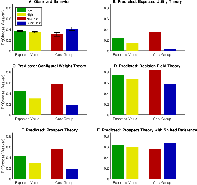
Figure 3: Observed data and predicted results from 5 different models, separated by factor. The vertical axis shows the probability of choosing a weaker option, separated by factor. The factors are expected value (low vs. high) and cost group (no vs. sunk). The predictions displayed for all of the models were generated using typical parameter values (see appendix for details). Prospect theory with the shifted reference point was able to account for the ordinal pattern in the observed data. Error bars in panel A represent standard error of the mean (for expected value factor, the error bars are the standard error of the mean difference between conditions). The data are separated by factors because the two main effects but not their interaction were significant. Importantly, note that the parameters used to generate these predictions were not optimized to the observed data.
Of primary importance is whether or not the Study 1 result was replicated when controlling for alternative explanations.7 The result did replicate. This was tested using a 2 x 2 mixed effects ANOVA, with cost group (no versus sunk) as a between-subjects factor and expected value (low versus high) as a within-subjects factor, resulting in two significant main effects (cost group: F(1,75) = 4.37, p < .05; expected value: F(1,75) = 4.08, p < .05). Those in the sunk cost group selected a stochastically dominated option significantly more than did those in the free group. Moreover, a novel finding was that people chose a stochastically dominated option significantly more when the trial’s expected value was low compared to when it was high (the mean probabilities of choosing a stochastically dominated option across the four condition by group cells are presented in Figure 3A). Although the difference in probabilities for choosing a stochastically dominated option between expected value conditions was normally distributed, the probability distributions for choosing a stochastically dominated option in the no cost and sunk cost groups were not. We therefore further analyzed this data using a nonparametric Mann-Whitney U test, which also indicated a statistical difference between the two payment groups for the probability of choosing a stochastically dominated option (z = 2.1, p < .05).
Next, we wanted to determine whether any of the models that have previously accounted for violations of stochastic dominance [i.e., prospect theory with and without a shifted referent point (Kahneman & Tversky, 1979), configural weight theory (Birnbaum & Navarrete, 1998), and decision field theory (Diederich & Busemeyer, 1999)] could account for this pattern of results. The predictions of these four models using typical parameter values, together with those of expected utility theory, are shown in Figure 3B-F.8 As Figure 3 clearly demonstrates, all five of these models yield ordinally correct predictions of the expected value main effect by successfully predicting that violations of stochastic dominance decrease as expected value increases. However, all except prospect theory with the shifted reference point yield ordinally incorrect predictions of the cost main effect, as each predicts that violations of stochastic dominance decrease as sunk costs increase.
Given that these theories are all mathematically instantiated, their parameter values can actually be optimized to the data. So we did this by minimizing the negative log likelihood of each model, given the observed marginal choice probabilities over all subjects using fminsearch in Matlab. We chose to fit over all subjects instead of at the individual subject level because the latter would have proven trivial for the models to fit. It is the mismatch in behavior between the two cost groups that was most challenging to fit, a challenge that was encountered only between subjects. The number of free parameters for each model, together with their fitness values according to the Bayesian Inference Criterion (BIC; Schwarz, 1978), are displayed in Table 2 (see the appendix for model formulas and additional model fitting information including the best fitting parameter values). Each of these models outperformed a 0-parameter baseline model which had a BIC of 25,619. As indicated by its having the lowest BIC value, prospect theory with the shifted reference point is again the single best model, even after adjusting for the number of free parameters. Hence, both the ordinal and model fitting comparisons suggest that incorporation of the risk attitudes and loss by shifting the reference point best accounts for the role of sunk costs in producing stochastic dominance violations.
Table 2: Number of free parameters and fitness values separated by model.
Note: The lower the BIC value the better the fit. See the appendix for additional fit details, best fitting parameter values, and computation of the BIC. BIC = Bayesian Information Criterion.
The results of two studies indicate that individuals are more likely to violate the stochastic dominance principle when in a sunk cost situation and when the expected value is low compared to high (Study 2). Interestingly, while all five models naturally predicted the effect of expected value, none except for prospect theory with the shifted reference point were able to predict the effect of sunk costs.
Several conclusions can be inferred from the results. First, these two new observations of stochastic dominance violations in individual choice complement previous observations of the violations such as when the dominance is non-transparent and in cases where payoffs are negatively correlated (Birnbaum & Navarrete, 1998; Diederich & Busemeyer, 1999; Tversky & Kahneman, 1986). Second, that violations of stochastic dominance decrease as expected value increases is not surprising. This corresponds with the finding that, as the stakes are raised, so raised is the attention and care exercised, also known as the speed/accuracy trade-off (Busemeyer & Townsend, 1993; Link, 1992; Ratcliff, 1978). However, the fact that stochastic versions of the formerly deterministic models captured this phenomenon is somewhat surprising because there is nothing within these implementations that changes with expected value; nonetheless, the observed behavior “falls out” quite effortlessly. It should be noted that the effect size for the expected value effect is small, though nonetheless statistically significant.
Third, the fact that sunk costs result in increased selection of a stochastically dominated option when compared to no costs is also surprising. It contradicts the apparent implications of the speed/accuracy trade-off, since, in this condition, the stakes are raised by the required investment. The predictions of the stochastic versions of these deterministic models again correspond to our incorrect intuitive expectations and hence they counter the observed behavior. Even the very flexible models that we tested were unable to account for these effects. Only with the incorporation of a shifted reference point together with the kinked valuation curve was a model able to capture the observed four-fold ordinal behavior pattern of expected value and cost group.
The observed pattern of results cannot be explained by probability matching, randomness, loss aversion as implemented within prospect theory, or the loss attention hypothesis which states that losses increase the likelihood of selecting the most advantageous option (Yechiam & Hochman, 2013). Contrastingly, in our results, subjects who experienced losses (i.e., sunk cost group) were less – not more – likely to choose the most advantageous option. Furthermore, because the d’, or sensitivity index, for each of the conditions and groups was held constant between the dominant and weaker options at 0.2108, the pattern also cannot be explained by the payoff variability effect (i.e., the finding that choices become more random as the d’ approaches zero; Busemeyer & Townsend, 1993; Myers, Suydam & Gambino, 1965). In the present case, the payoff variability effect would predict no choice difference between the expected value conditions or investments groups. Thaler and Johnson (1990) suggest that riskier choices might be more prevalent when subjects are influenced by prior positive outcomes. Individuals in their experiment were more risk-seeking after experiencing an initial gain. These “house money” affects cannot explain the stochastically dominated choices being investigated here because subjects do not receive a positive endowment or an initial gain before making choices.
An important caveat to note is that the work here involved situations in which sunk cost is forced; it remains to be seen if the effect holds when subjects have free choice concerning whether or not to engage in the sunk cost task. Furthermore, the extent to which the effect depends on having more than two options might also be examined in future work. The synthesis of our present work with the finding that individuals are more likely to violate stochastic dominance than groups (Charness, Karni & Levin, 2007) suggests that the problem of inferior decision making by executives who act alone will be exacerbated when there are costs on the line, a problem that might be ameliorated by having many outside and independent advisers involved in the decision making process.
To summarize, prior research has shown that individuals choose irrationally in the presence of sunk costs. This research presents a novel connection between sunk costs and stochastic dominance. The effect of sunk costs on choices that contain dominated options was not predicted by any pre-existing deterministic model of choice using reasonable parameter values without a change of reference. Financial investment in the form of a sunk cost results in changes to an individual’s reference point, affecting his or her likelihood of choosing a stochastically dominated option. In the case of our experiment, these poor choices had only minimal consequences; in the case of the London Whale, the consequences were anything but minimal. The novelty of the present findings, when viewed through the lens of real-world human behavior, open new avenues for interesting future research.
Abdellaoui, M., Bleichrodt, H., & l’Haridon, O. (2008). A tractable method to measure utility and loss aversion under prospect theory. Journal of Risk and Uncertainty, 36(3), 245–266.
Arkes, H. R., & Blumer, C. (1985). The psychology of sunk cost. Organizational Behavior and Human Decision Processes, 35(1), 124–140. http://doi.org/10.1016/0749-5978(85)90049-4.
Birnbaum, M. H., & Chavez, A. (1997). Tests of theories of decision making: Violations of branch independence and distribution independence. Organizational Behavior and Human Decision Processes, 71(2), 161–194. http://doi.org/10.1006/obhd.1997.2721.
Birnbaum, M. H., & McIntosh, W. R. (1996). Violations of branch independence in choices between gambles. Organizational Behavior & Human Decision Processes, 67(1), 91–110. http://doi.org/10.1006/obhd.1996.0067.
Birnbaum, M. H., & Navarrete, J. (1998). Testing descriptive utility theories: Violations of stochastic dominance and cumulative independence. Journal of Risk and Uncertainty, 78, 49–78.
Birnbaum, M. H., Patton, J., & Lott, M. (1999). Evidence against rank-dependent utility theories: Tests of cumulative independence, interval independence, stochastic dominance, and transitivity. Organizational Behavior and Human Decision Processes,[ 77(1), 44–83. http://doi.org/10.1006/obhd.1998.2816.
Busemeyer, J. R., Jessup, R. K., Johnson, J. G., & Townsend, J. T. (2006). Building bridges between neural models and complex decision making behaviour. Neural Networks[202F?]: The Official Journal of the International Neural Network Society, 19(8), 1047–58. http://doi.org/10.1016/j.neunet.2006.05.043.
Busemeyer, J. R., & Townsend, J. T. (1993). Decision field theory: a dynamic-cognitive approach to decision making in an uncertain environment. Psychological Review, 100(3), 432–459. http://doi.org/10.1037/0033-295X.100.3.432.
Charness, G., Karni, E., & Levin, D. (2007). Individual and group decision making under risk: An experimental study of Bayesian updating and violations of first-order stochastic dominance. Journal of Risk and Uncertainty, 35(2), 129–148. http://doi.org/10.1007/s11166-007-9020-y.
De Martino, B., Kumaran, D., Seymour, B., & Dolan, R. J. (2006). Frames, biases, and rational decision-making in the human brain. Science, 313(5787), 684–687.
Diederich, A., & Busemeyer, J. R. (1999). Conflict and the stochastic-dominance principle of decision making. Psychological Science, 10(4), 353–359. http://doi.org/10.1111/1467-9280.00167.
Ditterich, J., Mazurek, M. E., & Shadlen, M. N. (2003). Microstimulation of visual cortex affects the speed of perceptual decisions. Nature Neuroscience, 6(8), 891–898. http://doi.org/10.1038/nn1094.
Gold, J. I., & Shadlen, M. N. (2007). The neural basis of decision making. Annual Review of Neuroscience, 30, 535–574. http://doi.org/10.1146/annurev.neuro.29.051605.113038.
Green, D. M., & Swets, J. A. (1966). Signal detection theory and psychophysics. New York: Wiley.
Hurtado, P. (2016). The London Whale. Retrieved May 24, 2018, from http://www.bloombergview.com/quicktake/the-london-whale.
Jessup, R. K., Bishara, A. J., & Busemeyer, J. R. (2008). Feedback produces divergence from prospect theory in descriptive choice. Psychological Science, 19(10), 1015–1022. http://doi.org/10.1111/j.1467-9280.2008.02193.x.
Jessup, R. K., & O’Doherty, J. P. (2011). Human dorsal striatal activity during choice discriminates reinforcement learning behavior from the gambler’s fallacy. The Journal of Neuroscience, 31(17), 6296–6304. http://doi.org/10.1523/JNEUROSCI.6421-10.2011.
Kahneman, D., & Tversky, A. (1979). Prospect Theory: An Analysis of Decision under Risk. Econometrica, 47(2), 263–292. http://doi.org/10.2307/1914185.
Levy, H., & Levy, M. (2002). Experimental test of the prospect theory value function: A stochastic dominance approach. Organizational Behavior and Human Decision Processes, 89(2), 1058–1081.
Link, S. W. (1992). The wave theory of difference and similarity. Hillsdale, NJ: Lawrence Erlbaum Associates.
Luce, D. (1959). Individual choice behavior: A theoretical analysis. New York: John Wiley and Sons.
Machina, M. J. (1989). Dynamic consistency and non-expected utility models of choice under uncertainty. Journal of Economic Literature, 27(4), 1622–1668.
Myers, J. L., Suydam, M. M., & Gambino, B. (1965). Contingent gains and losses in a risk-taking situation. Journal of Mathematical Psychology, 2(2), 363–370.
Navarro, A. D., & Fantino, E. (2005). The sunk cost effect in pigeons and humans. Journal of the Experimental Analysis of Behavior, 83(1), 1–13. http://doi.org/10.1901/jeab.2005.21-04.
Quiggin, J. (1982). A theory of anticipated utility. Journal of Economic Behavior and Organization, 3(4), 323–343.
Ratcliff, R. (1978). A theory of memory retrieval. Psychological Review, 85(2), 59–108. http://doi.org/10.1037/0033-295X.85.2.59.
Roe, R. M., Busemeyer, J. R., & Townsend, J. T. (2001). Multialternative decision field theory: A dynamic connectionst model of decision making. Psychological Review, 108(2), 370–392. http://doi.org/10.1037/0033-295X.108.2.370.
Schwarz, G. (1978). Estimating the dimension of a Model. The Annals of Statistics, 6(2), 461–464. http://doi.org/10.1214/aos/1176344136.
Strough, J., Mehta, C. M., McFfall, J. P., & Schuller, K. L. (2015). Are older adults less subject to the sunk-cost fallacy than adults? Psychological Science, 19(7), 650–652.
Sutton, R. S., & Barto, A. G. (1998). Reinforcement learning: an introduction. IEEE Transactions on Neural Networks / a Publication of the IEEE Neural Networks Council, 9(5), 1054. http://doi.org/10.1109/TNN.1998.712192.
Tan, H.-T., & Yates, J. F. (1995). Sunk cost effects: The influences of instruction and future return estimates. Organizational Behavior and Human Decision Processes, 63(3), 311–319.
Thaler, R. H., & Johnson, E. J. (1990). Gambling with the house money and trying to break even: The effects of prior outcomes on risky choice. Management Science, 36(6), 643–660. http://doi.org/10.1287/mnsc.36.6.643.
Tversky, A., & Kahneman, D. (1986). Rational choice and the framing of decisions. The Journal of Business, 59(S4), 251–278. http://doi.org/10.1086/296365.
Tversky, A., & Kahneman, D. (1992). Advances in prospect theory: Cumulative representation of uncertainty. Journal of Risk and Uncertainty, 5(4), 297–323. http://doi.org/10.1007/BF00122574
Von Neumann, J., & Morgenstern, O. (1944). Theory of games and economic behavior. Princeton University Press.
Yechiam, E., & Hochman, G. (2013). Loss-aversion or loss-attention: The impact of losses on cognitive performance. Cognitive Psychology, 66(2), 212–231. http://doi.org/10.1016/j.cogpsych.2012.12.001.
Zeng, J., Zhang, Q., Chen, C., Yu, R., & Gong, Q. (2013). An fMRI study on sunk cost effect. Brain Research, 1519, 63–70. http://doi.org/10.1016/j.brainres.2013.05.001.
Expected utility theory (Von Neumann & Morgenstern, 1944) represents the simplest descriptive model of choice behavior. The expected utility of an option k with J outcomes is given by
| EUk = |
| pj u(xj) , (1) |
where pj represents the probability of outcome j and xj is the value of outcome j and u is a function that converts the outcome to utility. We used a standard reference dependent power function for utility,
| u(xji) = | ⎧ ⎨ ⎩ |
| , (2) |
where α is a utility parameter that indicates an individual’s attitude towards risk. When α > 1, an individual is risk-seeking; α < 1 indicates risk aversion, and α = 1 indicates risk neutrality, reducing the model to expected value. To produce Figure 3B we used α = .81 to account for the common finding that individuals are risk averse in the gain domain. The optimization process for the two free parameters yielded α = .01 and θ = .078 (see obtaining probabilistic predictions from deterministic models section in the appendix for explanation of the θ parameter).
Configural weight theory (Birnbaum & Chavez, 1997; Birnbaum & McIntosh, 1996) has proven to be an extremely successful model at explaining effects not predicted by cumulative prospect theory and it excels at accurately predicting stochastic dominance violations. According to this model, the preference for an option k with two outcomes x and y where x > y ≥ 0 is given by
| CWT(xk) = wH u(x) + wL u(y) , (3) |
where u(• ) represents the standard power function for utility with utility parameter α , and the relative weight wH on the high outcome x is given by
| wH = |
| . (4) |
Here, aH and aL are configural weights that for the high and low outcomes, respectively, S(•) represents a probability weighting function of the form pγ. The relative weight for the lowest outcome wL = 1−wH. To produce Figure 3C the parameter values were aH = .37, aL = 1 − aH, α = 1, γ = .6 (Birnbaum & Chavez, 1997). The optimization process for the four free parameters yielded aH = 1, α = .01, γ = 2, and θ = .01. Parameter aL was fixed at 1 - aH. Unfortunately, when the options have binary outcomes configural weight theory produces predictions virtually indistinct from those of cumulative prospect theory (Birnbaum & Chavez, 1997; Birnbaum & McIntosh, 1996). Nonetheless, because this is a very flexible model that has successfully accounted for previous violations of stochastic dominance, we still wanted to see if it could predict the observed effects.
Decision field theory is a dynamic and stochastic model of choice that has found a wide variety of application in both traditional behavioral decision making literature, and, owing to its neural network structure and similarity with neural behavior (Ditterich, Mazurek & Shadlen, 2003; Gold & Shadlen, 2007), has managed to bridge the behavioral literature with the neuroscience literature (Busemeyer, Jessup, Johnson & Townsend, 2006). There are multiple versions of this model for both binary and multi-alternative choice, including models with both externally- and internally-controlled stopping times. Predictions were generated using both stopping time approaches and they yielded qualitatively identical answers. Because it has known solutions, we are using the externally-controlled stopping rule version (Roe, Busemeyer, & Townsend, 2001) for the model fitting procedure as opposed to the internally-controlled version which must be simulated.
In decision field theory, preferences for options are accumulated until they reach a predetermined decision threshold θ . The accumulation of preference in this model is best described using matrix notation and preferences at time t accumulate according to
| P(t) = S· P(t−1) + V(t) , (5) |
where P represents a preference vector of length K, where K = the total number of options; S is a K by K feedback matrix; and V(t) is a valence vector of length K, representing the valence for each option at each moment. The main diagonal coordinates sii in the feedback matrix allow for decay and the off-diagonal coordinates allow for lateral inhibition of competing alternatives. The valence vector is described by
| V(t) = C· M· w(t) + N(0,σ) , (6) |
where C is a K by K comparison matrix; M is a K by J motivational matrix, representing the J options outcomes for each option k on the columns; w(t) is an attentional weight vector of length J; and N(0,σ ) is a normally distributed noise factor with a mean drift rate of 0 and standard deviation of σ , representing the diffusion rate. For a more in-depth treatment of the model, see Roe et al. (2001). The predictions shown in Figure 3D were obtained using 5000 simulations for each condition and group combination (i.e., 2 · 2 · 5000 = 20,000 total simulations) with the following parameter values: sii = 1, θ = 4, σ = .05; the lateral inhibition parameter connecting the high probability to the low probability options shigh_low = slow_high = −.05; and the lateral inhibition parameter connecting the two low probability options slow_low = −.1. The optimization process for the four free parameters yielded θ = 50, σ = 2.0, shigh_low = slow_high = −.16, and slow_low = −.06. The feedback parameter was not fit but rather fixed at sii = .95.
Prospect Theory (Kahneman & Tversky, 1979) represents a major advance beyond expected utility that is able to capture a wide variety of choice patterns that expected utility theory cannot.
The prospect V for option k is defined as
| Vk = |
| π(pj)· v(xj) (7) |
where v(xj) represents the S-shaped value function from a neutral reference point for option x and outcome xjj. In practice, this was implemented according to
| u(xi) = | ⎧ ⎨ ⎩ |
| , (8) |
where α is a utility parameter for gains and β is a utility parameter for losses. The loss aversion parameter λ is a multiplier that increases the impact of losses relative to equivalent gains. The probability weighting function for positive outcomes π+(pj) is used to modify the probability p of each outcome j and is operationalized according to (Tversky & Kahneman, 1992)
| π+(pj) = |
| , (9) |
where γ is a probability weighting parameter such that γ < 1 yields overweighting of rare events, γ > 1 yields underweighting of rare events and γ = 1 yields objective weighting of rare events. The probability weighting function for negative outcomes π−(pj) is identical in form except that a different free parameter δ is used in place of γ . In accordance with Tversky and Kahneman (1979), the weighted probabilities need not sum to unity. To produce Figure 3E the parameter values used were α = β = .88, γ = .61, δ = .69, and λ = 2.25 (Tversky & Kahneman, 1992). The optimization process for the six free parameters yielded α = .01, β = 2, γ = .36, δ = .01, λ = .01, and θ = .01.
This version is identical to prospect theory except that, when losses are the default (e.g., in the sunk cost group), the maximum outcome is subtracted from all outcomes. This allows the maximal outcome to become the new origin for the kinked value function.
| xj − MAX(x) for all j , (10) |
The parameters used to produce Figure 3F were the same as those used to produce 3E. The optimization process for the six free parameters yielded α = .11, β = .14, γ = 2, δ = .57, λ = 2, and θ = .06.
Expected utility theory, prospect theory, and configural weight theory all make deterministic predictions, unlike decision field theory. Given that individual – much less group – behavior is not deterministic, it is essential that some mechanism be used to convert the deterministic predictions into probabilistic predictions. The softmax implementation (Sutton & Barto, 1998) of the Luce choice rule (Luce, 1959) is a commonly used conversion method. Our particular version is computed as follows:
| pk = |
| . (11) |
Here, Pk represents the probability of selecting option k out of the set of K options, Mk represents the value from the deterministic model (whether a utility or prospect) for option k, and θ represents the temperature parameter on the range 0 < θ < ∞. Our formulation uses the inverse of the temperature parameter so that values near 0 result in more deterministic choice behavior whereas increases in θ result in increasingly random choice behavior. We used θ =.02 to produce the results displayed in Figure 3 for all deterministic models.
The Bayesian Information Criterion (BIC) is a model comparison method that can be used to compare multiple non-nested models. The BIC is computed as
| BICi = −2· LLi + ln(N)· k , (12) |
where LLi represents the (natural) log likelihood of model i, N is the number of data points or observations, and k is the number of free parameters in the model. The term after the plus sign can be thought of as a penalty for added model complexity, represented by the number of free parameters. In study 2, each additional free parameter within a model adds a penalty value of ln(77· 240) = 9.824 because we optimized over all 77 subjects and each subject had 240 trials. The lower the BIC value, the better the fit.
To insure that our models were performing better than chance we compared them to a 0-parameter baseline model that makes the simplifying assumption that each of the 77 subjects chose the dominant option 50% of the time over all 240 trials. The log likelihood of this model is ln(.5) · 77 · 240 and the BIC value of this model is simply −2 · LLBaseline = 25,619. In order to outperform this baseline model – and consequently yield a lower BIC value – the subjects must choose in ways that systematically deviate from chance behavior and a competing experimental model must efficiently detect and adjust accordingly to these deviations. A 0-parameter baseline model that chose the dominant option either 40% of the time – to correspond with probability matching – or 33% of the time – to correspond with pure guessing – would have fared even worse than the version we used.
We would like to thank Kyle Tippens for thoughtful discussion, Chelsea Flow for help creating figures, John O’Doherty for letting us use the behavioral choice data from Jessup & O’Doherty (2011) as well as from their unpublished pilot studies, and grants from the ACU Cullen Foundation and Office of Undergraduate Research.
Copyright: © 2018. The authors license this article under the terms of the Creative Commons Attribution 3.0 License.
This document was translated from LATEX by HEVEA.