Judgment and Decision Making, Vol. 11, No. 5, September 2016, pp. 424-440

Two experiments explored how the context of recently experiencing an abundance of positive or negative outcomes within a series of choices influences risk preferences. In each experiment, choices were made between a series of pairs of hypothetical 50/50 two-outcome gambles. Participants experienced a control set of mixed outcome gamble pairs intermingled with a randomly assigned set of (a) all-gain, (b) all-loss, or (c) a mixture of all-gain and all-loss gamble pairs. In both experiments, a positive experience led to reduced risk taking in the control set and a negative experience led to increased risk taking. These patterns persisted even after the all-gain and all-loss gamble pairs were no longer present. In addition, we showed that the good luck attributed to positive experiences was associated with decreased, rather than increased, risk taking. These results ran counter to the house money effect, and could not readily be accounted for by changes in assets. We suggest that the goals associated with the predominant valence are likely to be assimilated and applied to other choices within a given situation. We also discuss the need to learn more about the characteristics of choice bracketing and mental accounting that influence which aspects of situational context will be included or excluded from consideration when making each choice.

Keywords: risk, choice, experience, context, assimilation, valence, positive, negative, gamble, goals

1  Introduction

Good and bad experiences form an essential part of the context of everyday life. These experiences may influence subsequent behavior and may be especially important when they form the context for situations involving some level of risk or uncertainty. For example, a person who has recently experienced several positive outcomes across a series of risky or uncertain events might feel differently about taking a risk than someone who has just experienced several negative outcomes. The purpose of this research is to explore how recent good and bad experiences in succession are likely to influence people’s tendencies to approach or avoid risks.

1.1  Reference points and risk taking

The importance of the valence of outcomes forms a cornerstone of prospect theory (Kahneman & Tversky, 1979). Its S-shaped value function separates option outcomes according to whether they are perceived as gains or losses relative to some reference point, often assumed to be the status quo. Generally speaking, risk preferences are predicted to reverse (or shift) based on whether the outcomes are perceived as gains or losses. This prediction forms the basis of two well-known and very commonly observed effects: the reflection effect and the framing effect. In both effects, preferences tend to be risk averse for outcomes perceived as gains, but risk seeking for outcomes perceived as losses. These differences in risk preferences have been replicated in a number of studies of risky choice (see, e.g., Kuhberger, Schulte-Mecklenbeck & Perner, 1999; Levin, Schneider & Gaeth, 1998), consistently demonstrating the impact of good and bad outcomes on preferences.

However, the predictions of prospect theory are generally limited to an evaluation of the prospect itself (including the presentation context or framing of that prospect) without consideration of recent related experiences or the broader surrounding context of any particular event. In fact, because the reference point is typically set to one’s current position (i.e., status quo), prospect theory suggests that the broader context is often ignored by routinely resetting one’s point of reference to disregard recent good or bad experiences and by focusing instead on the current state. Exactly how and when the reference point will be reset is left open within prospect theory, but the general tendency to focus on the present state is often seen as one of the descriptive strengths of prospect theory’s reference dependent approach (e.g., Starmer, 2000; Tversky & Kahneman, 1981, 1991).

1.2  Context sensitivity in risky choice

Although the recognition of reference dependence and the impact of outcome valence on choice has contributed greatly to our understanding of risky decision making, it may distract attention from broader contextual impacts associated with enjoying a set of good experiences or suffering a set of bad ones. What happens when things are getting worse and worse, or better and better? In their review of findings related to the construction of preferences, Warren, McGraw and Van Boven (2011) contend that context sensitivity is a ubiquitous aspect of all cognition and behavior, and thus can be expected to influence virtually all preferences and choices. Among the most commonly identified underpinnings of context sensitivity are goals, which change as the situation changes.

Any number of studies, ranging from investigations of changing aspiration levels (e.g., Lopes, 1987; Wang & Johnson, 2012) to contrast effects in consumer choice (e.g., Simonson & Tversky, 1992; Tversky & Simonson, 1993) suggest that as the situation changes, our perceptions of acceptable outcomes also change. This interplay between reference dependence and goals suggests that decision makers are likely to be especially sensitive to situations in which things are regularly improving or deteriorating. In this study, we explore how a series of good or bad experiences may alter one’s tendency to seek or avoid risks.

Previous research on the influence of good and bad experiences on subsequent risk taking has typically focused on how a single previous gain or loss may influence gambling behavior. The classic example is the work of Thaler and Johnson (1990), who examined how prior gains and losses affected risk taking in a variety of gambling scenarios. They found that people were more willing to take a risk after they had just experienced a gain. They called this finding the house money effect. They suggested that, after a gain, people see themselves as “ahead” and dealing with “house money” instead of their own money. Until the “house money” is gone, subsequent losses are coded as reductions in gains. After a loss, in most cases, people tended to decrease their willingness to take a risk, except when the risky option held some promise of winning back, and thus negating, the prior loss. In that case, termed the break even effect, people are more apt to be risk seeking in an attempt to win back what they had lost.

Thaler and Johnson (1990) observed that neither standard expected utility theory nor prospect theory could straightforwardly account for their findings. Although the editing operations posited in prospect theory seemed promising, the pattern of results depended on the specific context in ways not addressed in the theory. Thaler and Johnson suggested the possibility of a quasi-hedonic editing principal which suggests that a prior gain will most often result in a shift in the risk seeking direction whenever losses can be re-coded as reduced gains, and that a prior loss will shift preferences in a risk-averse direction to minimize the potential for future losses, unless the outcome of taking the risk might allow the decision-maker to fully recover the amount previously lost. Similarly, Barberis, Huang & Santos (2001) suggested that investors in the stock market tend to be less loss averse (i.e., more risk seeking) after a gain because the gain cushions any subsequent loss, but more loss averse after a loss given the sense that further losses cannot be tolerated.

Consistent with these predictions, Ma, Kim and Kim (2014) found that online gamblers tended to increase gambling after a win and to reduce gambling after a loss. Similarly, Kostek and Ashrafioun (2014) found that participants playing blackjack wagered more after winning a majority of five previous hands than after losing a majority.

Weber and Zuchel (2005), however, found only weak evidence in support of the pattern of increased risk taking after gains and decreased risk taking after losses, and only in a presentation format involving a two-stage betting game rather than a decision about a portfolio. When participants thought about their series of decisions as part of a larger portfolio, the opposite pattern was observed wherein risk taking was more likely to increase after a loss than after a gain. Franken et al. (2006) also found greater risk taking after a loss than a gain. They manipulated initial gains and losses within gamble sets using the Iowa Gambling Task (IGT). They found that, when participants’ first round of the task yielded a gain, they gravitated more quickly toward the less risky options than those whose first round resulted in a loss.

One characteristic of all of these tasks is that winning or losing the gamble is inextricably tied to whether one experiences a gain or loss. Thus, experienced outcomes influence not only earnings, but also the sense that one has been lucky or unlucky. So, in Thaler and Johnson (1990), for instance, people might have been more willing to take a risk after they won, not because they had extra money but because the win made them feel lucky (or perhaps a combination of the two). They may even have interpreted the win as providing information about the likelihood of winning or losing in upcoming gambles (e.g., Ball, 2012; Croson & Sundali, 2005; Leopard, 1978).

1.3  Separating earnings from likelihoods

In the current investigation, we remove the possible confound between changes in earnings and the experience of obtaining the better or worse outcome (i.e., winning or losing) in a gamble. We do this by presenting participants a series of choices between two-outcome gamble pairs in which the chance of getting the better or worse outcome is always 50/50, but the expected value of a manipulated subset of gamble pairs is categorically positive for some participants and negative for others. We then ask whether risk taking in a control set of lotteries changes as surrounding outcomes become routinely positive or routinely negative, despite the fact that all participants obtain the better outcome in their chosen gambles roughly half of the time and the worse outcome the other half.

If the house money effect is driven by a process such as quasi-hedonic editing, and the idea that having extra money allows one to be able to afford the risk of a loss, then our findings should be similar to those of Thaler and Johnson. In that case, we would anticipate increased risk taking in the positive environment and decreased risk taking in the negative environment (at least until one’s earnings have been depleted). On the other hand, if other factors such as perceptions of luck or changing outcome expectations are important drivers of the effect, then the patterns might be weaker when earnings are not primarily dependent on whether one wins the gamble.

Studies by Huber (1994, 1996) suggest that the pattern of our results might even be opposite those of Thaler and Johnson. In a series of multistage investment tasks, Huber separately manipulated likelihood of winning and amounts that could be won. He found that the higher likelihood of winning increased the relative size of wagers (i.e., people took larger risks), but that greater increases in earnings were generally associated with decreases in the relative size of wagers (i.e., people took smaller risks). With investments, this suggests that there are opposing forces at work, with higher likelihood of winning encouraging risk-taking behavior and higher earnings discouraging risk-taking behavior. In our studies, we examined whether this pattern would be replicated in the context of risky choice. Specifically, Huber’s findings lead to the prediction that, when likelihood of winning is held constant, people will make more risk averse choices when they have recently experienced positive events that have increased their earnings, and will make more risk seeking choices when they have recently experienced negative events that have decreased their earnings.

1.4  Toward understanding characteristics of context

Another consideration involves possible differences in the strength of context effects. Arkes et al. (2008), for instance, reported an asymmetry in reference point adaptation as a function of upturns versus downturns in stock prices. They showed that reference points typically shift more, or are more likely to be reset, after gains than after losses. This result suggests that a context with mostly positive events may have relatively little effect on preferences because the context is effectively ignored by resetting the reference point. In contrast, a context of negative events may have larger effects on preferences because the surrounding context is more likely to continue to exert an influence on upcoming choices.

Following Shefrin & Statman (1985), Imas (2016) has suggested that resetting the reference point is often synonymous with closing the mental account associated with ongoing gains or losses. He argues that a single mental account is likely to be maintained until paper earnings are realized; for example, when a stock or other asset is sold. He hypothesized that ongoing (non-realized) paper losses would create a narrow frame (Kahneman & Lovallo, 1993) or choice bracket (Read, Loewenstein & Rabin, 1999; Thaler, 1999) inclusive of the non-realized outcomes, but exclusive of any other assets. Thus, with non-realized losses, choices in the non-realized choice bracket or mental account would be integrated and evaluated jointly, while ignoring all other sources of wealth. In contrast, once losses are realized, the integration process within the choice bracket would be predicted to stop, the net gain or loss would be internalized, and the reference point for the mental account would be reset.

In support of this, Imas (2016) showed that experiencing a paper loss across a series of investments in an experimental task led to an increase in risk taking represented by larger investments over time, whereas realizing the loss was associated with a decrease in the amount invested on a subsequent trial. He also demonstrated that the results of other similar studies were consistent with the hypothesis of increased risk taking after paper losses (Langer & Weber, 2008) and decreased risk taking after realized losses (Shiv et al., 2005). These findings are consistent with the differences in preferences for choices in two-stage gambles versus portfolios reported by Weber & Zuchel (2005).

These findings also suggest a link between the literature on mental accounting effects and context effects, potentially shedding light on when the larger decision making context is more likely to generate assimilation versus contrast effects. According to Bless and Schwarz’ (2010; Schwarz & Bless, 1992) inclusion/exclusion model, information that is incorporated into the representation of the decision results in assimilation effects, whereas information that is excluded from the representation supports contrast effects. If the larger context is assimilated, new choice options would be reviewed as reductions or increases to previous amounts won or lost. All else equal, this suggests that a positive environment would make new choice options seem more positive, and a negative environment would make new choice options seem more negative. On the other hand, a contrast effect would exaggerate the differences between the surrounding context and the choice option. Thus, a positive environment might make (less good) choice options seem more negative than otherwise, and a negative environment might make (less bad) choice options seem more positive than otherwise. In sum, assimilation effects would lead to preferences that are consistent with those in the surrounding valence (i.e., increased risk aversion in positive conditions and increased risk seeking in negative conditions), whereas contrast effects would lead to preferences that look more like those of the opposite valence.

Imas’ (2016) findings suggest that the decision making context is likely to be defined by the active mental account. With paper losses, assimilation effects would be most likely, as the context would include previous related investments. Generalizing beyond investments, this yields the prediction that the positive or negative context created by outcomes in a series of risky choices is more likely to yield assimilation when the series is connected by monetary results that are not realized within the series. However, the house money effect and the quasi-hedonic editing hypothesis (Thaler & Johnson, 1990) suggest that this single mental account will increase risk taking in the positive domain, not decrease it. We test these competing hypotheses in two experiments.

2  Experiment 1: Risk taking for gambles surrounded by positive versus negative events

In the first experiment, we examine how a situational context marked by a series of good versus bad experiences may influence risky choice, particularly when those good or bad experiences are not tied to the likelihood of winning. To do this, we elicit preferences for a set of control 50/50 gamble pairs with expected values near zero when they are embedded in a larger set that consists of (a) 50/50 gamble pairs with only positive outcomes, (b) 50/50 gamble pairs with only negative outcomes, or (c) a mixture of 50/50 all positive and 50/50 all negative gamble pairs. Our goal is to resolve conflicting hypotheses about whether good versus bad outcome experiences, independent of likelihood of winning, increase or decrease tendencies to take risks.

Following the logic of Thaler and Johnson’s (1990) house money effect, those who have had recent good outcomes have more money available within the gambling context and so should feel more open to taking risks, whereas those who have had recent bad outcomes should be less willing to risk their depleting resources. In contrast, if recent good and bad outcomes are seen more as earnings on investments, then results may be more in line with Huber’s findings (1994, 1996), with increased earnings leading to a decrease in risk-taking tendencies and reduced earnings leading to an increase in risk-taking behavior. The latter finding would also be consistent with Imas’ (2016) hypothesis that the non-realized losses in a series of risky choices promote risk taking through mental accounting and associated narrow framing processes. Our design also allows us to assess whether this prediction can be generalized to gains with the prediction of enhanced risk aversion consistent with an assimilation effect (Bless & Schwarz, 2010).

We also evaluate whether there are asymmetries in the influence of positive and negative events on risky choice. If the results of Arkes et al. (2008) generalize to this situation, effects of negative experiences would be expected to be stronger than the effects of positive experiences, as the reference point would be less likely to be reset after negative experiences.

---

Table 1: Example of gamble pairs from the control, positive experience, negative experience, and mixed experience sets.

Gamble set		EV		Variance	Higher-risk gamble		Lower-risk gamble
					Lower outcome	Higher outcome	Lower outcome	Higher outcome
NEG, MIX2		–$200		MEDIUM	–$275	–$125	–$225	–$175
CONTROL		$0		LOW	–$50	$50	$0	$0
CONTROL		$0		HIGH	–$100	$100	–$50	$50
POS, MIX1		$200		MEDIUM	$125	$275	$175	$225
Notes: EV = Expected Value, NEG = Negative experience set, POS = Positive experience set, MIX1 = Mixed experience set (first subset), MIX2 = Mixed experience set (second subset).

---

2.1  Method

2.1.1  Participants

We used an online system to recruit 111 undergraduate students from a large urban university. They participated anonymously for psychology course credits. Twenty nine participants were later removed from analysis — 25 participants due to failure to pass an eight-item quiz testing attention to and understanding of the stimuli and 4 participants due to computer problems.¹ Useable data were provided by 82 participants. An additional 124 participants were randomly assigned to another task, the results of which will be reported elsewhere.

---

Figure 1: Three-block pre-post manipulation study design. The control set of 18 gamble pairs was repeated in each block. Only the second (manipulation) block included the additional 18 gamble pairs from the randomly assigned positive, negative, or mixed experience condition. The three blocks were completed as an undifferentiated set of 72 gamble pairs in one of four random orders.

[t]1.5inBlock1
(Pre-manipulation)  =⇒  [t]1.5inBlock2
(Manipulation)  =⇒  [t]1.5inBlock3
(Post-manipulation)

[t]2in18 control gamble pairs
EV: –$50 to $50[t]2in18 control gamble pairs
EV: –$50 to $50
Randomly mixed in with …
Negative EV: –$75 to –$200
or
Mixed EV: –$75 to –$200 AND $75 to $200
or
Positive EV: $75 to $200[t]2in18 control gamble pairs
EV: –$50 to $50

---

2.1.2  Stimuli and materials

Each trial consisted of a choice between a pair of hypothetical 50/50 two-outcome gambles that shared the same expected value. The riskier gamble was defined as the gamble with the higher variance, or greater deviation in outcomes (e.g., Lopes, 1987; Yates & Stone, 1992).

Four sets of 18 gamble pairs were created: the control set and three experience sets. A sample of these gamble pairs is shown in Table 1. The control set was structured according to a 2x3x3 Valence x (absolute) Expected Value x Variability design to create a variety of choices involving gambles with a mixture of positive, zero, and negative outcomes. The valence of each gamble pair was either positive or negative. Expected values were $0, $25 or $50. Variability was low, medium, or high and corresponded to the separation in the two outcomes within a gamble, with a larger separation corresponding to greater risk. The lower risk gamble in a pair had outcome separations of $0, $50, or $100, and the higher risk gamble had outcome separations of $100, $150, or $200 based on whether the gamble pair was low, medium, or high variability, respectively.

The positive and negative experience sets were both structured according to a 6x3 Expected Value x Variability matrix to create choices involving all gains or all loss outcomes. Expected values of the positive experience set ranged from +$75 to +$200 in increments of $25. Expected values of the negative experience set ranged from –$75 to –$200. Variability was manipulated for gamble pairs in both sets just as in the control set.

To create the mixed experience set, the positive and negative experience gamble pairs were carefully split into two equivalent halves. One half from each set was combined so that each positive and negative expected value was represented at least once, and the three variability levels were each experienced 6 times, distributed as evenly as possible across expected values. The combined expected value of the mixed experience set of 9 positive and 9 negative gamble pairs was within ±$25. Because creating one mixed experience set automatically yielded a second equivalent set of “leftover” gamble pairs, we used both sets by randomly counterbalancing which one of them was experienced by each participant in the mixed experience condition.

2.1.3  Design

The experiment utilized a 3x3 Experience x Block mixed design depicted in Figure 1. An undifferentiated set of 72 gamble pairs were presented in one of four random orders. The control set of 18 gamble pairs was presented once each in the pre-manipulation, manipulation, and post-manipulation blocks. Only the manipulation block (Block 2) also included 18 interspersed gamble pairs from the randomly assigned experience condition. In each block, the primary dependent variable was the number of times the riskier gamble was chosen within the 18 gamble pairs of the control set.

---

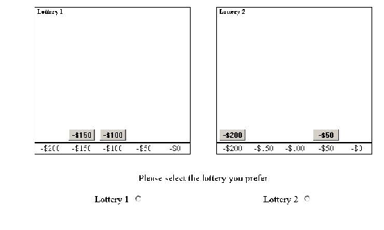
Figure 2: Example of a gamble pair as presented on the computer screen. Depicted are two lotteries, each with the same expected value of –$125. Each gamble has two equally likely tickets, each labeled with the outcome that would be received if the ticket were randomly chosen when played. In this example, Gamble 1 represents the safer option; Gamble 2 represents the riskier option. Participants were instructed to choose the gamble in each pair that they would prefer to play by clicking the corresponding radial button below the gamble.

---

Two open-ended questions were also included at the end of the study to corroborate the impact of the experience manipulation: “Did you do better or worse than expected on the task?” and “How do you feel about how well you actually did in the task? Please explain”. For exploratory purposes, participants were also prompted to report the strategies they used throughout the experiment.

2.1.4  Procedure

Participants were given free choice of seating in a 12-seat computer laboratory. After consent, participants received a pen as a thank-you gift. They were told that whether or not they could keep it, as well as earn an additional prize, were dependent upon performance in the experiment. The experimenter then delivered the instructions, during which participants learned about the final totals required to keep the pen ($1,250) and to earn an additional prize ($2,500). They also learned about the representation of gambles as two tickets on a number line. They were instructed to choose the gamble that they preferred to play out of each gamble pair, an example of which is provided in Figure 2.

Participants then began the self-administered portion of the experiment, beginning with the eight-question quiz to assess understanding of the gambles and their associated probabilities. Starting with a balance of $1,250, the 3 blocks of gamble pairs were then played as an undifferentiated set of 72 gamble pairs. On each trial, after choosing the preferred gamble, the gamble would be played. This occurred via an animated pair of dice that would roll momentarily, after which the preferred gamble re-appeared on the screen with the randomly selected ticket highlighted and the current total updated accordingly. This running total was maintained at the top of the computer screen throughout the experiment so that participants were aware of their current earnings. The participant proceeded to the next trial at his or her own pace.

After completing the gamble choice task, the three open-ended questions were presented. Before each participant left the laboratory, they saw the experimenter individually. At this time, the participant “cashed in” or realized their results in that they received an additional prize (a candy bar) or returned the gift pen to the experimenter depending on their final earnings on the gamble choice task.

---

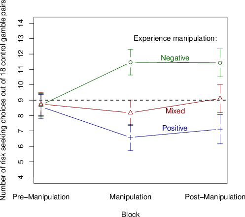
Figure 3: Experience x Block interaction effect on risk taking in Experiment 1. The experience manipulation gamble pairs were only present in the manipulation block. Average standard error bars are displayed. The dashed horizontal line in the center of the graph separates a predominance of risk averse preferences (lower area) from a predominance of risk seeking preferences (upper area).

---

2.2  Results

The influence of the experience manipulation on risk preferences was assessed by analyzing the number of risks taken across the control set of 18 gamble pairs before, during, and after the manipulation. A 3x3 Experience x Block mixed ANOVA was performed to determine the influence of surrounding positive or negative experiences on risk taking.²

2.2.1  Analysis of control set preferences

There was a significant main effect of experience, F(2,79)=3.97, p=.023, partial η ²=.09. In contrast to the findings of Thaler and Johnson (1990) but consistent with those of Huber (1994, 1996), participants with a positive experience took the fewest risks within the control set of gambles and those with a negative experience took the most risks. There was no main effect of block, F(2,158)=1.64, p=.20, but there was a significant Experience x Block interaction, F(4,158)=10.96, p<.001, partial η ²=.22, which is shown in Figure 3.

---

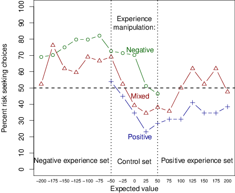
Figure 4: Percentage of risk seeking choices for experience conditions in Experiment 1’s manipulation block. Expected values for gamble pairs in the control set ranged between ±50 whereas those for experience manipulation gamble pairs ranged from ±75 to ±200 depending on condition. The dotted lines in the mixed experience condition serve as a reminder that participants saw only half of the gamble pairs at that expected value.

---

Participants in all conditions began the experiment by taking roughly the same number of risks in the pre-manipulation block (F<1). During the transition from the pre-manipulation through the manipulation block, those having a negative experience began taking more risks across the control set, t(27)=–4.00, p<.001; d=0.76, while those having a positive experience began taking fewer risks across the control set, t(25)=2.30, p=.03; d=0.49. Those with a mixed experience did not significantly change in their risk taking, t(27)=1.11, p=.28, n.s. In the post-manipulation block, the pattern continued, providing evidence for an enduring effect even when the positive and/or negative experience gambles were no longer present. These results suggest that having the experience of doing well, despite winning and losing about equally often, tends to decrease willingness to take risks in subsequent more neutral situations, with the opposite effect for those having the experience of doing poorly.

2.2.2  Breakdown of manipulation block

In order to better understand the effect of experience on risk preferences, a closer look at the risk preference patterns in the manipulation block was taken. We wanted to see how participants responded to the gamble pairs in the experience sets compared to the gamble pairs in the control set. Figure 4 displays the risk preference patterns in the manipulation block for each experience condition. Specifically, Figure 4 presents the proportion of times participants were risk seeking for each expected value in the manipulation block, averaging over the variance manipulation. The middle portion of the figure labeled ‘Control Set’ includes the Block 2 data that were analyzed in the previously described ANOVA. As reported there, those with a negative experience took the most risks, followed by those with a mixed, and then positive, experience. These choices were made in response to the control set, which contained gamble pairs with expected values near zero (from –$50 to +$50). Expanding left and right from the control set, Figure 4 also displays the risk preferences for the positive and negative experience gamble sets. The dotted lines in the mixed experience condition represent the fact that participants saw only half of the gamble pairs.

As would be predicted by Kahneman and Tversky’s (1979) prospect theory value function, participants tended to be risk seeking when making choices among negative experience gambles (all-loss outcomes), but tended to be risk averse when choosing among positive experience gambles (all-gain outcomes). Preferences for the control gamble pairs seem to be “pulled” in the same direction so that risk seeking was more common in the control set when combined with a negative experience, but considerably less common when combined with a positive experience.

Thus we observed a pattern consistent with an assimilation process rather than one suggestive of a contrast effect (e.g., Bless & Schwarz, 2010). Being surrounded by positive experiences led responses to the (less good) control gambles to become more like responses to all-gain gambles, not the reverse. In fact, the extent of risk aversion in the positive experience condition during Block 2 was comparable for the control set and the all-gain gambles, t(25)=0.35, p=.73, n.s. In complementary fashion, when surrounded by negative gambles, responses to the (less bad) control set became more like responses to all-loss gambles. This is consistent with Imas’ (2016) predictions for non-realized losses. Despite being pulled in that direction, however, risk taking in the control set was not as extreme as in the negative experience set, t(27)=3.51, p=.002, d=.66. This suggests that, if anything, the positive experience had the larger influence on risk taking in the control set, which is opposite what was observed by Arkes et al. (2008).

Comparison of the all-loss and all-gain gamble preferences across the different experience conditions provides additional evidence of the effect of context (Figure 4). Preferences for the experience gambles seem less extreme within the mixed condition than in the consistent valence conditions. Among the all-gain gambles, those with a consistently positive experience took significantly fewer risks than those with a mixed experience when making choices within the all-gain gamble pairs, t(52)=2.10, p=.04, d=.57. For the all-loss gambles, there appeared to be a tendency for those with a consistently negative experience to take more risks in the all-loss pairs than those with a mixed experience, although the difference only approached significance, t(54)=1.89, p=.065, d=.50 . Thus, experiencing the same valence of outcomes repeatedly seems to enhance the risk-taking patterns within the larger set. This pattern provides corroborating evidence of the influence of a consistent positive or negative surround in solidifying risk-taking tendencies.

2.2.3  Manipulation checks

The experience manipulation was successfully corroborated using the responses to the two open-ended questions. For those in the positive experience condition, 92% reported that they did better than expected, and 85% felt good about how they did. In contrast, 86% of those assigned to the negative experience condition reported that they did worse than expected, and 71% felt poorly about how they did. Those in the mixed experience condition fell in between, with 32% (57%) reporting that they did better (worse) than expected and 25% (43%) felt good (poorly) about how they did. Thus, respondents were aware of the larger context.

The use of the running total and prizes to emphasize the experience to participants also demonstrated the impact of the experience manipulation. The average final current totals for those with positive, mixed, and negative experiences was $3,809, $1,235 and –$1,172, respectively. Of those with a positive experience, all but one participant kept their pen and received the candy bar. All participants with a mixed experience kept their pen, but did not earn enough for a candy bar. Of those with a negative experience, all but one participant lost their pen.

3  Experiment 2: Online replication

Results from Experiment 1 suggested that good outcome experiences that are not associated with luck (or probability of obtaining the better outcome in a gamble) tend to decrease tendencies to take risks, whereas bad outcome experiences tend to increase risk taking. Consistent with an assimilation effect, being exposed to all-gain gambles seemed to pull preferences for more neutral gambles in a risk averse direction, whereas exposure to all-negative gambles caused a gravitation to risk seeking preferences among the control gambles. These results are inconsistent with the house money effect and the break even effect (given that risk seeking was observed routinely in the negative experience condition even when there was no chance of recovering what had been lost). Instead, results are more in line with Huber’s (1994, 1996) investment findings, suggesting that increases in earnings tend to reduce risk taking, whereas reductions in earnings are more likely to increase risk taking (see also Imas, 2016).

One alternative to this possibility is that the pen and candy prizes in Experiment 1 might have created an unintended incentive system for conserving earnings once the “prize” levels had been reached, or “going for broke” when below the prize levels. To rule out this possibility, we conducted an online replication study without any prizes.

We also included an exploratory measure to assess attributions about the role of luck in the task. If experiences of luck are closely tied to the likelihood of getting the better or worse outcome, then there should be virtually no differences in luck attributions across experience conditions. On the other hand, if attributions of luck are mainly tied to the relative preponderance of good or bad outcomes, regardless of whether they correspond to obtaining the better or worse outcome in the gamble, then we would expect to see large differences in luck attributions between the positive and negative experience conditions. Such a result, combined with a replication of the Study 1 results, would imply that feeling lucky can support risk averse rather than risk seeking behavior.

---

Table 2: Four-item luck attribution scale anchors.

Positive endorsement of luck	Negative endorsement of luck
I feel that the odds were in my favor.	I feel that the odds were against me.
I was lucky in my lottery outcomes.	I was unlucky in my lottery outcomes.
Overall I was lucky.	Overall I was unlucky.
I feel my score is due to good luck.	I feel that my score is due to bad luck.

---

3.1  Method

3.1.1  Participants

Using the same online system as in the original study, 161 undergraduate students were recruited. Those who had participated in the previous study were not permitted to participate in the replication. Of the 161 participants, 55 were excluded from the analysis for failure to pass the quiz testing attention to and understanding of the gambles.³ An additional 4 were excluded due to excessive missing data, leaving 102 participant response sets for analysis.

3.1.2  Stimuli and design

The same gamble sets in the same four random orders from Experiment 1 were re-used for the replication study, and the design was nearly identical. Although a running total of the participants’ earnings was again visible throughout the study, one critical difference was that no prizes or other incentives were awarded based on score. Participants were simply instructed that the goal of the task was to accumulate as much money as possible.

All measures used in the original study were included in the online replication. In addition, several pilot measures being tested for use in later studies were added at the end of this study. One of these was a four-item luck attribution scale designed to measure subjective assessments of whether one has been experiencing good or bad luck across a series of gamble pairs. Face-valid items were created on a five-point Likert-type scale with opposing anchor statements on each side of the scale, as seen in Table 2. A ‘1’ indicated agreement with the leftmost statement, whereas a ‘5’ indicated agreement with the rightmost statement.

---

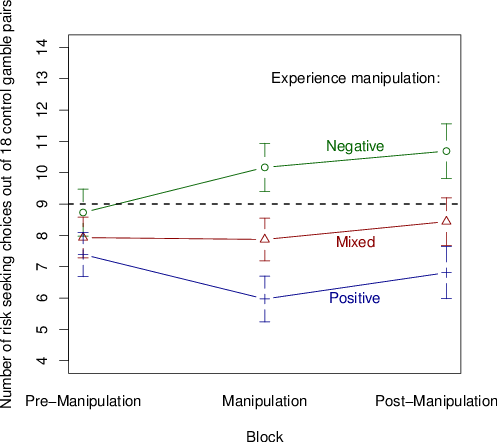
Figure 5: Experience x Block interaction effect on risk taking in Experiment 2. The experience manipulation gamble pairs were present only in the manipulation block. Average standard error bars are displayed. The dashed horizontal line in the center of the graph separates a predominance of risk averse preferences (lower area) from a predominance of risk seeking preferences (upper area).

---

3.1.3  Procedure

The study was made available online to psychology undergraduates so that participants could complete the study from any computer with internet access. Participants were randomly assigned to one of the three experience conditions. Online instructions explaining the nature of the study and how to choose between the gamble pairs were followed by the eight-item quiz assessing the participant’s understanding of the task. The pre-manipulation, manipulation, and post-manipulation blocks of gamble pairs were then presented, and on each trial, participants watched as their chosen gamble was played and their accrued earnings were updated based on the outcome. When the gamble portion of the study was finished, participants completed the pilot measures followed by the open-ended questions from the original study.

3.2  Results

The results of the 3x3 Experience x Block mixed ANOVA are shown in Figure 5. As in the original study, we again observed a main effect of experience, F(2,99)=4.95, p=.009, partial η ²=.09, and a significant Block x Experience interaction, F(3,158)=3.90, p=.009, partial η ²=.07 (Greenhouse-Geisser correction applied). As in Experiment 1, participants in the negative experience condition took significantly more risks within the control set than those in the positive experience condition, with the mixed condition falling in between. As in Experiment 1, participants started with no differences in risk-taking preferences in the pre-manipulation block, F(2, 99)=.85, p=.43, n.s. During the manipulation block, there was a substantial increase in risk taking for control gamble pairs in the negative experience condition, t(29)= 3.40, p=.002, d=.63, and a sizable decrease in risk taking in control gambles for those in the positive experience condition, t(32)= 2.57, p=.015, d=.45, with no discernable change in the mixed experience condition, t(38)=.011, p=.92, n.s. In the post-manipulation block, even when the positive or negative gambles were no longer present, the changes in risk-taking patterns persisted. Thus, the findings from Experiment 1 were fully replicated.

Responses to the open-ended manipulation check items again corroborated the effects of the experience manipulation: 76% of those in the positive experience condition reported that they did better than expected, and 85% felt good about how they did; in contrast, 83% of those assigned to the negative experience condition reported that they did worse than expected, and 43% admitted that they felt they did poorly. Those in the mixed experience condition were in between, but unlike those in Experiment 1, were more similar to the positive experience condition, with about 62% reporting that they did better than expected and 67% reporting that they felt good about how they did. Average final earnings were $3,755, $1,467, and –$1,080 for the positive, mixed, and negative experience conditions, respectively.

We also took an exploratory look at responses to the four-item Luck Attribution Scale to see whether participants would attribute their good or bad outcomes across the experiment to luck, even though the probability of winning versus losing (i.e., getting the better versus worse outcome of the gamble) in all conditions was 50/50 throughout. Reliability among the four items was quite high, Cronbach’s α =.83, so the items were combined into a single index with scores ranging from –8 = very unlucky to +8 = very lucky.

The results of a one-way ANOVA revealed large differences in luck attribution scores across experience conditions, F(2,99)=32.71, p<.001, η ²=.39. Tukey post-hoc tests showed that luck attribution scores in the positive (M=+2.39, SD=2.55) and mixed experience (M=+1.23, SD=2.25) conditions were significantly higher (p<.001) than scores in the negative experience condition (M=–3.23, SD=3.18). These results suggest that participants in both the positive and mixed experience conditions felt that they experienced mild good luck, whereas those in the negative experience condition felt that they had experienced mild to moderate bad luck. The link between earnings and luck attributions was unmistakable in the correlation between the two, r(102) = .64, p<.001, showing that higher earnings were associated with attributions of good luck. Remarkably, then, perceptions of luck were driven by the valence of outcomes and not the likelihood of obtaining the better or worse outcome within gamble plays. Moreover, the perceived good luck from positive experiences was associated with increased risk aversion, not increased risk taking.

---

Table 3: Percent preferring the risk within the positive and negative experience conditions for each control gamble pair within each of the three blocks of trials.

Gamble Pair		Block 1: Pre-manipulation				Block 2: Experience manipulation				Block 3: Post-manipulation
		Experience				Experience				Experience
EV	Variance	Neg.	Pos.	ϕ	Sig	Neg.	Pos.	ϕ	Sig	Neg.	Pos.	ϕ	Sig
–$50	Low	83%	80%	.04		63%	61%	.02		67%	61%	.06
–$50	Medium	57%	54%	.03		66%	44%	.22	*	72%	54%	.18
–$50	High	78%	59%	.20	*	78%	54%	.25	*	78%	53%	.26	**
–$25	Low	74%	75%	–.01		78%	58%	.21	*	84%	59%	.29	**
–$25	Medium	86%	78%	.11		86%	46%	.42	**	79%	46%	.35	**
–$25	High	31%	34%	–.03		53%	20%	.34	**	60%	34%	.26	**
$0	Low	60%	54%	.06		69%	29%	.40	**	57%	34%	.23	*
$0	Medium	38%	41%	–.03		62%	25%	.37	**	66%	37%	.28	**
$0	High	43%	34%	.09		66%	27%	.39	**	72%	31%	.42	**
$0	Low	59%	47%	.11		62%	36%	.26	**	62%	34%	.28	**
$0	Medium	33%	39%	–.06		66%	29%	.37	**	72%	46%	.27	**
$0	High	41%	34%	.08		67%	36%	.32	**	76%	34%	.42	**
$25	Low	36%	24%	.14		33%	17%	.18		24%	20%	.05
$25	Medium	24%	20%	.05		40%	14%	.30	**	36%	24%	.14
$25	High	38%	34%	.04		67%	41%	.27	**	62%	41%	.21	*
$50	Low	41%	43%	–.02		55%	49%	.06		60%	47%	.13
$50	Medium	29%	34%	–.05		43%	24%	.21	*	38%	24%	.15
$50	High	19%	8%	.15		28%	15%	.15		38%	17%	.24	*
	Average:	48%	44%			60%	35%			61%	39%
Note. N per test = 57–59; Neg. = Negative, Pos. = Positive, EV = Expected Value; * p<.05, ** p<.01.

---

4  General discussion

The purpose of these experiments was to explore the relationship between general positive and negative contexts and risky decision making. We were especially interested in differentiating good and bad experiences from winning and losing per se. The experience of good and bad outcomes did have an influence on participants’ risk preferences, but the resulting patterns were opposite of the house money effect found by Thaler and Johnson (1990). Across the two studies, a nominal count showed that 82% of the participants in the positive experience conditions shifted risk taking in the direction of decreasing the number of risks taken after the control block. In the negative experience conditions, 71% of participants shifted towards ncreased risk-taking. Participants in the mixed experience were about even in their propensity to increase (49%) or decrease (46%) risk taking.

These findings were in line with those of Huber (1994, 1996) who found that increasing capital was associated with decreases in the relative size of wagers. Our results were also consistent with an assimilation process rather than a contrast effect (e.g., Bless & Schwarz, 2010). The results were also congruent with Imas’ (2016) finding that paper losses, in contrast to realized losses, tend to promote risk seeking in an attempt to avoid previously incurred losses.

Of particular interest, the observed patterns of preferences continued even when the positive and negative experience gambles were no longer present. We found that participants were well aware of the larger context, and that they associated luck with these experiences, even though they faced 50/50 probabilities throughout. Surprisingly, we showed that the good luck attributed to positive experiences was associated with decreased, rather than increased, risk taking.

---

Table 4: Percent within Block 1 preferring the risk on the subsequent gamble pair as a function of previous outcome.

Gamble Pair		Relative status				Absolute status
		Previous outcome				Previous outcome
EV	Variance	Worse	Better	ϕ	Sig	Loss	Gain	ϕ	Sig
–$50	Low	76%	83%	.09		80%	78%	–.02
–$50	Medium	59%	66%	.07		56%	58%	.01
–$50	High	81%	66%	–.17	*	75%	66%	–.09
–$25	Low	78%	77%	–.02		81%	81%	–.01
–$25	Medium	91%	73%	–.23	*	92%	75%	–.16
–$25	High	37%	31%	–.06		37%	31%	–.06
$0	Low	62%	59%	–.03		57%	57%	.00
$0	Medium	40%	34%	–.05		40%	34%	–.05
$0	High	35%	40%	.05		77%	39%	–.18	**
$0	Low	55%	55%	.01		50%	58%	.08
$0	Medium	56%	55%	–.01		56%	34%	–.21	*
$0	High	40%	30%	–.10		40%	33%	–.07
$25	Low	32%	25%	–.08		32%	25%	–.08
$25	Medium	28%	16%	–.14		27%	16%	–.13
$25	High	49%	26%	–.24	**	66%	26%	–.38	**
$50	Low	43%	40%	–.03		39%	43%	.04
$50	Medium	35%	28%	–.07		34%	44%	.08
$50	High	13%	22%	.12		13%	22%	.12
	Average:	51%	46%	–.05		53%	46%	–.06
Note. EV = Expected Value; * p<.05. For worse/better, Ns ranged from 68 to 184. For loss/gain, Ns ranged from 99 to 184.

---

4.1  The generality of the effect of positive and negative experience across control gambles

Before considering the possible explanations for the changes in average preferences across the 18 control gamble pairs, we first wanted to determine the extent to which the context effect influenced each of the individual gamble pairs. To do this, we combined the data across the two studies and examined whether preferences among each of the control pairs differed significantly as a function of being surrounded by a set of highly positive or negative gambles. The results for each of the three blocks of trials are presented in Table 3.

As shown in the left-hand columns, we confirmed that preferences for the various gambles did not differ in Block 1 which occurred prior to the experience manipulation. The single significant difference out of 18 pairs is roughly what would be expected by chance. However, during the manipulation block (Block 2), shifts in aggregate preferences were found for 14 of the 18 gamble pairs, and shifts in preferences continued to be evident for 12 of the 18 gamble pairs in the post-manipulation block (Block 3). The effect was weakest among the gamble pairs with a positive expected value, although in all cases, the differences were in the expected direction. Thus, we confirmed the generality of the pattern of increased risk taking after a negative experience and decreased risk taking after a positive experience.

4.2  The potential role of previous outcome in changing risk preferences

Several aspects of our positive and negative experience manipulations might contribute to their influence on risk preferences. The house money and break even effects (Thaler & Johnson, 1990), for instance, are based on the assumption that winning or losing a gamble directly influences one’s willingness to take a risk at the next opportunity (e.g., Croson & Sundali, 2005). As a follow up, we investigated this hypothesis in both relative and absolute terms. That is, we combined data across the two studies looking at preferences for each control gamble from Block 1 (before the experience gambles had been presented), and separately examined risk taking based on whether the previous outcome had been the better or the worse of the two possible outcomes in the gamble, or whether the previous outcome had been a gain or a loss. This was an exploratory analysis with some overlap between the two comparisons, and some cases in which the previous outcome was a sure thing (so that better or worse was inapplicable) or zero (so that gain or loss was inapplicable). Thus, the numbers in each comparison change somewhat across the gamble pairs. The findings from this exploratory analysis are presented in Table 4.

As shown in the table, there is little evidence that the status of the previous outcome, either in relative or absolute terms, was a primary determinant of risk-taking tendencies on the next gamble. Across the 18 control gambles, there were only 3 instances in which preferences seemed to differ systematically based on whether the prior outcome was the worse versus better outcome and only 3 instances in which preferences seemed to differ based on whether the prior outcome was a loss versus a gain (which is only slightly more than would be expected by chance).

It is noteworthy, however, that the results of all 6 cases went in the direction opposite of what would be predicted by the house money effect. In each case, receiving the better or gain option was associated with less rather than more risk taking on the next gamble pair. Moreover, ϕ exceeded 0.1 in less than one third of cases (11 of 36), but when it did, it was in the direction of less risk taking for better or gain outcomes in all but two cases. Thus, there was little evidence that the previous outcome was especially influential in encouraging or discouraging risk taking, but, when it was, its effects were opposite of expectations based on the house money effect.

Thus, Thaler and Johnson’s (1990) quasi-hedonic editing hypothesis cannot account for our results. For those having a positive experience, their increase in earnings would make it easier and easier to be able to “afford” taking the risk. That is, the quasi-hedonic editing hypothesis predicts that these participants would view any loss as a reduced gain in earnings, and therefore should have been more willing to take a risk. However, we found the reverse to be true. Experiencing a preponderance of positive outcomes led to a decreased willingness to take a risk. According to the quasi-hedonic editing hypothesis, risk aversion should be more typical for those having a negative experience, unless they have the opportunity to recoup their recent losses. We found instead a steady increase in risk taking as negative outcomes accumulated. Rather than observing a break-even effect, we observed what seems more like a desperation effect, in which participants became increasingly despairing as their resources dwindled to nothing or dropped below zero. Indeed, a review of the strategy comments of negative experience participants revealed examples consistent with this possibility, such as: “At a certain point I had nothing left to lose so I just went for it,” and “Once I got to a point where I didn’t think I could get to a positive value again I gave up and chose the ones that had the higher reward.” These comments provide some qualitative support for the proposal by Imas (2106) that people tend to maintain a single mental account within a series of “paper” transactions and that, after losses, they become focused on minimizing the size of the cumulative loss before it is realized.

---

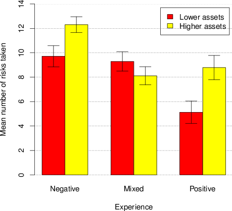
Figure 6: Experience x Asset Level interaction effect on risk taking in Experiments 1 and 2 combined. Higher and lower asset levels were calculated based on median splits of the average amount of assets, by experience, in Block 3. For the negative, mixed, and positive experience conditions, respectively, averages for the higher asset groups were –$739, $1692, $4162, and averages for the lower asset groups were –$1556. $1063, $3417. Average standard error bars are displayed.

---

4.3  The potential role of assets in changing risk preferences

We were also interested in investigating the possibility that overall assets were the primary driver of our results, as might be expected based on the results of studies by Huber (1994, 1996). On the face of it, our results seem more in line with those of Huber, who found that larger capital gains in an investment task were associated with relative decreases in amounts wagered. Their findings suggest that the accumulation of earnings may be a critical factor in explaining why surrounding negative and positive outcomes lead to more and less risk taking, respectively. In our studies, then, higher asset values would be expected to be associated with less risk taking. Because asset values were unavoidably confounded with our experience manipulation, we examined the relationship between assets and preferences within each experience condition, again combining the data from Studies 1 and 2.

We first separated the data into 9 Block x Experience conditions and computed the average assets for each individual within the block. We then computed the correlations between average assets for each individual within each block and number of risks taken within the control set of gambles in that block. Correlations ranged from –.16 to .22, and were not significant in any of the 9 conditions (with average asset standard deviations of $204, $540, and $730, respectively, in Blocks 1–3). However, the use of correlations in this context might not adequately capture any asset-risk taking relationship, as those who take more risks are more likely to experience extreme outcomes (and thus asset positions). In light of this, we also used median splits to separate participants into those with higher versus lower average assets within Block 3, wherein differences among asset positions was greatest. If assets are the primary driver of our results, we would expect to see that those with higher average assets tend to take fewer risks than those with lower average assets. The results of this analysis are presented in Figure 6.

Figure 6 shows the differences in control set risk taking that were reported in Block 3 of both studies with more risk taking in the negative experience condition and less risk taking in the positive experience condition. Within two of the three conditions, we also observed differences in risk taking as a function of assets. Contrary to predictions of the influence of assets (Huber, 1994, 1996), in both the negative and the positive experience conditions, those with higher average assets took more risks than those with lower average assets, t(56)=2.37, p<.05, d=.62, and t(57)=2.70, p<.01, d=.70, respectively. No differences in risk-taking preferences based on asset level were observed in the mixed experience condition, t(65)=1.08, n.s. Thus, the overall tendency for experience to shift preferences toward risk aversion when in a positive situation and toward risk seeking in a negative situation cannot be readily explained as a phenomenon driven directly by asset level. If anything, higher asset levels (more positive or less negative) were associated with greater rather than less risk taking. Thus, local preference patterns were opposite of what Huber found for investment amounts.

4.4  The potential role of goals in changing risk preferences

Our results show that the prevailing context of gains versus losses is more apt to lead to assimilation effects than contrast effects. After positive experiences, an option with mixed outcomes seems more positive, whereas after a negative experience, the same mixed-outcome option seems more negative. In some ways, this seems surprising. After seeing a series of all-gain gambles, the presence of a choice between two mixed-outcome prospects in the control condition might have seemed relatively negative, enhancing participants’ risk-taking tendencies. After a series of all-loss gambles, the mixed-outcome prospects might have seemed relatively positive, discouraging risk taking. Instead, the results seem to show a gradual “pull” of control set preferences in the direction of the predominant strategy associated with the typical valence of options. Thus, our results shed some light on how decisions may be influenced by the larger contextual surround.

Nevertheless, it is not simply that people were blindly carrying over their predominant response from the experience gambles to the control gambles. We correlated risk-taking responses for the experience lotteries with the change in risk taking for the control gambles from the first to the second block. We found only modest relationships [r(57)=.23, p=.08 for positive experience and r(56)=.30, p=.02 for negative experience], suggesting that more is needed to explain these results.

Based on participants’ manipulation check responses, we showed that the prevailing context is likely to be (1) cognitively coded as a good or bad situation, (2) predictably linked to positive or negative expectations, and (3) affectively evaluated as doing well or doing poorly. Not surprisingly, the good or bad valence associated with the preponderance of recent experiences was associated with both affective and goal-related responses to the situation (e.g., Heath, Larrick & Wu, 1999; Lerner et al., 2015; Loewenstein et al., 2001; Mellers et al., 1999). With respect to the establishment of reference points and the related construction of preferences, these types of context-based responses are likely to play a critical role in the development of ongoing decision goals. Without an impetus to reset the reference point, such as realizing earnings (Imas, 2016), the role of context may be especially powerful.

In their review of findings concerning preference construction, Warren et al. (2011) concluded that changing goals are particularly potent contextual influences on the construction of preferences. Context influences both goal accessibility (Bless & Schwarz, 2010; Van Osselaer et al., 2005) and goal activation (Markman & Brendl, 2000). In the context of risk taking, goals associated with achieving potential versus security (Lopes, 1987; Schneider & Lopes, 1986) or focusing on approach versus avoidance (Heath, Larrick & Wu, 1999) are likely to be differentially salient depending on the surrounding positive or negative context.

In general, positive situations may encourage attention to staying positive, whereas negative situations may focus attention on getting out of the negative situation. Isen and colleagues’ mood maintenance hypothesis (e.g., Isen & Patrick, 1983; Isen, Nygren & Ashby, 1988), for instance, might suggest that those who are having a positive experience would want to maintain any associated positive affect by refraining from taking a risk. Those having a negative experience might try to remedy the associated negative affect by taking a risk in order to move toward a more positive affective state. Thus, positive experiences may reinforce goals that provide a means of safely moving forward, whereas negative experiences may shift attention toward avoidance strategies that ultimately tend to move choices in a risk-seeking direction. Thus, a predominance of positive or negative experiences may generate a kind of attentional or goal drift that influences the way that risky choices are evaluated, not only among the clearly bad and good events, but also among proximate events.

Consistent with this possibility, March and Shapira (1987) reported that managers generally believe that fewer risks should be taken when things are going well. In their review of two studies involving over 500 executives from three different countries, they concluded: “Both the managers interviewed by Shapira and those interviewed by MacCrimmon and Wehrung (1986) believe that fewer risks should, and would, be taken when things are going well. They expect riskier choices to be made when an organization is “failing …Most managers seem to feel that risk taking is more warranted when faced with failure to meet targets than when targets were secure.” (p. 1409).

Particularly in Experiment 1, participants could have been viewing their situation as going well or poorly with respect to reaching external goals provided within the task. When participants were having a positive experience, or were in a strong position, they might have viewed taking risks as potentially compromising their already high status. In their view, they already were getting a prize and keeping their pen, so there was no need to jeopardize that by taking risks. Consider, for example, the following strategy volunteered by one of the positive experience participants: “I stuck to playing it safe unless I had enough to where it didn’t matter if I lost 500, as long as I had 2500+ to get the prize”. Having a negative experience, however, might have gradually elicited risk-seeking tendencies because it was the only way that participants would have any shot at keeping their pen.

This possibility seems less convincing in Experiment 2, wherein participants had no goal other than achieving the highest total possible. Perhaps anchors such as the status quo at the outset ($1,250) and the transition point between assets and liabilities ($0) could have served a similar function as the prizes. If so, these kinds of anchors or reference points are likely to be important in a variety of contexts, and may allow for a better understanding of how contexts influence preferences under risk (e.g., Wang & Johnson, 2012). Positive and negative contexts are likely to inform the development of reference points by providing a sense of what is possible or realistic in a situation. Lopes (1987; Schneider & Lopes, 1986) as well as Heath, Larrick and Wu (1999) have argued and provided evidence that negative situations typically require decision makers to set higher, harder to reach goals that can be reached only by taking more risks than they would otherwise. The surrounding experiences that create situational context, then, may serve as key inputs in scaling one’s expectations and goals. Thus, it may be necessary to take the larger context into account in order to understand how people decide when they do and do not wish to take a risk.

4.5  Limitations and future directions

Our studies provide evidence that positive and negative contexts have a potent influence on risk preferences, resulting in assimilation effects that can alter risk preferences based on the predominant valence of recently-experienced outcomes. Context was created by including all-gain or all-loss lotteries intermixed with a set of control lotteries. Thus, positive and negative context was confounded, as it typically would be, with an increase or decrease in overall assets, respectively. Providing this asset information to the participants was done in order to reinforce the experience of doing well or poorly. Nevertheless, this confound makes it more difficult to isolate the impact of changing assets versus other contextual influences on risk taking. Although we used an exploratory post-hoc analysis to try to rule out changing assets as the primary driver of our findings, a stronger demonstration would disentangle assets from our experience manipulation. Future studies, for instance, might remove feedback about assets, or manipulate the outcomes so that asset levels are manipulated independently.

Another area of interest concerns the robustness of context effects, and their relationship to establishing and working within a mental account or choice bracket. The work of Imas (2016) suggests that context effects are likely to be more robust when outcomes are not realized within a series of events. If so, our results might have been weaker or qualitatively different if outcomes were realized at various points within the series. These types of influences on resetting the reference point, and altering mental accounts or choice brackets, are likely to be critical to understanding what constitutes the relevant context and how that context may exert effects on risky choice.

Our studies were also confined to situations involving equiprobable outcomes. Another variant of positive and negative context would involve a higher or lower likelihood of receiving good and bad outcomes. The house money effect (Thaler & Johnson, 1990) as well as Huber’s findings (1994, 1996) suggest that the likelihood of better and worse outcomes in the surround may have different effects on risk preferences than exposure to positive and negative outcomes, per se. An especially surprising finding in Study 2 was that participants described themselves as lucky in the positive experience condition, while at the same time, they decreased their risk taking. This result is counterintuitive, and may point to a general tendency for people to conflate unexpected good experiences and probabilistically lucky events (e.g., Teigen, 1995; Teigen et al., 1999). Nevertheless, it remains to be seen whether behavior may be sensitive to shifts in the likelihood of better versus worse outcomes.

A related concern is whether, or how, outcomes are experienced. Studies have demonstrated a description-experience gap in which risk preferences can be shown to differ qualitatively based on whether risky prospects are simply described or whether their outcomes are experienced (e.g., Barron & Erev, 2003; Hertwig & Erev, 2009; Weber, Shafir & Blais, 2004). Experience provides feedback about obtained results as well as direct exposure to the variability in outcomes associated with particular probabilities. Many paradigms, including the one used here and many investment tasks, deviate from the typical description format by introducing some amount of feedback about outcomes. An understanding of the potential role of this type of outcome feedback is needed, along with an assessment of how the experience of a series of different prospects (as opposed to repeated experience with a single prospect) may contribute to differences in risky choice.

More broadly, future work will need to face the challenge of discriminating the many cognitive, motivational, and affective influences that are likely to affect preference construction. Positive and negative context are likely to bring about highly related sets of reactions including predictable changes in affect, attentional salience, goal accessibility, and goal activation. These influences are likely to combine with one another in the construction of preferences in any given setting. The development of more direct methods for manipulating, assessing, and discriminating these factors, including neuroscientific methods, may clarify how and when positive and negative context will impact risk-taking tendencies. Although neural correlates of the impact of positive and negative outcomes within gambles has now received considerable attention (e.g., Breiter et al., 2001; Rangel, Camerer & Montague, 2008), little attention has yet been given to the effects of the larger context within which risky choice may occur.

Doing relatively well or poorly is a ubiquitous part of experience. Our studies are focused on how changing the general valence of surrounding experiences can alter risk preferences for a given set of risky choices. In the two studies presented here, we have shown that being surrounded by positive outcomes tends to decrease tendencies to take on risk whereas a negative surround increases risk-taking tendencies. Thus, assimilation effects predominate, making risk-taking tendencies for any particular choice to be more similar to, rather than contrasting with, those of surrounding events. This result suggests that different goals are likely to become salient within a positive or negative environment and that preference construction is sensitive to these valence-based goals. Positive and negative context, then, is a potentially subtle yet important consideration in developing our understanding of influences on preference under risk.

5  References

*

University of South Florida, Department of Psychology, 4202 East Fowler Avenue, PCD4118G, Tampa, FL, 33620. Email: sandra@usf.edu.

#

University of South Florida

Copyright: © 2016. The authors license this article under the terms of the Creative Commons Attribution 3.0 License.

1

Analyses were also completed including data from those who failed the quiz. Results were virtually the same. All data are included in the online data.

2

Before any analyses were performed, 3 missing data points due to computer error were imputed. Preferences across the two equivalent mixed experience gamble sets were combined as they were virtually the same, F < 1.

3

Before any analyses were performed, 10 missing data points due to computer error were imputed. Analyses were also completed including data from those who failed the quiz. Results were virtually the same.

This document was translated from L^AT_EX by H^EV^EA.