Judgment and Decision Making, Vol. 12, No. 5, September 2017, pp. 430-444

People often perform poorly on stock-flow reasoning tasks, with many (but not all) participants appearing to erroneously match the accumulation of the stock to the inflow – a response pattern attributed to the use of a “correlation heuristic”. Efforts to improve understanding of stock-flow systems have been limited by the lack of a principled approach to identifying and measuring individual differences in reasoning strategies. We present a principled inferential method known as Hierarchical Bayesian Latent Mixture Models (HBLMMs) to analyze stock-flow reasoning. HBLMMs use Bayesian inference to classify different patterns of responding as coming from multiple latent populations. We demonstrate the usefulness of this approach using a dataset from a stock-flow drawing task which compared performance in a problem presented in a climate change context, a problem in a financial context, and a problem in which the financial context was used as an analogy to assist understanding in the climate problem. The hierarchical Bayesian model showed that the proportion of responses consistent with the “correlation heuristic” was lower in the financial context and financial analogy context than in the pure climate context. We discuss the benefits of HBLMMs and implications for the role of contexts and analogy in improving stock-flow reasoning.

Keywords: stock-flow reasoning, climate change, Bayesian models, mixture models

1  Introduction

Systems with a stock-flow structure involve an accumulating (or decreasing) stock that is determined by inflows and outflows. Such systems are common in business, public policy and everyday life. From warehouses, to the carbon cycle, to a standard bathtub, these systems have a common underlying mathematical structure. Formally, stock-flow problems belong in the domain of calculus. However, knowledge of the formal processes underlying stocks and flows may not be required to understand these concepts, or to solve simple stock-flow problems.

One apparently simple way to understand how stock-flow systems work is to imagine the water level in a bathtub (Booth Sweeney & Sterman, 2000; Cronin, Gonzalez & Sterman, 2009). If the water pouring from the tap is flowing at a greater rate than the water is draining out of the (unplugged) bathtub, then the water level will rise. Conversely, if the water is draining from the bathtub at a greater rate than it is flowing from the tap, the water level will fall. If the water is pouring into the bathtub at the same rate at which it is draining, then the water level will remain constant. More generally, the correct solution depends on the difference between inflows and outflows.

---

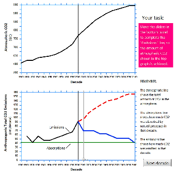
Figure 1: Screenshot of the CO2 drawing task adapted from Sterman and Booth Sweeney (2007). The task is to complete the emissions trajectory in the bottom graph so that the stabilization of atmospheric CO2 shown in the top graph is achieved. The solid blue sketched line in the bottom graph shows a correct response trajectory in which the emissions and absorption lines converge at the point of stabilization (2100). The red dashed line is a typical “correlation heuristic” response in which the emissions line mirrors the trajectory of the accumulation (i.e., continues steadily increasing). In our latent mixture model we describe participants who complete the lines in the lower panels by plotting an upward trajectory as “Up responders”, those who plot a downward trajectory as “Down responders” and those whose responses fit neither class as “Other responders”.

---

Despite the seemingly intuitive nature of this description, and the demonstrable fact that most of us know how to run a bath, experiments testing abstract reasoning about stock-flow systems have found that many people are unable to solve even simple stock-flow problems (Booth Sweeney & Sterman, 2000; Cronin et al., 2009; Sterman & Booth Sweeney, 2007). A consistent finding is that people frequently follow a “correlation heuristic” (Cronin, et al., 2009), whereby they infer that the stock of the system should be positively correlated with the inflow of the system. For example, if people are told or shown that the amount of water flowing into a bath is steadily increasing, they often infer that the level in the tub (the stock) will rise at a similar rate irrespective of the drainage rate – thereby positively correlating the inflow rate with the stock. Reliance on the correlation heuristic has been found to persist across manipulations of motivation, presentation format, and cognitive effort, suggesting that it is a robust cognitive error (Cronin, et al., 2009).

Failure to grasp the dynamics of stock-flows and the subsequent reliance on the correlation heuristic can have serious consequences. In the context of atmospheric CO₂ accumulation, for example, it is generally accepted that outflows (e.g., CO₂ absorption by carbon sinks) are likely to remain constant for the foreseeable future. Hence, increases in CO₂ emissions or maintenance of current emission levels will inevitably lead to a net increase in the accumulating “stock” of CO_2, which in turn will cause the temperature of the planet to rise. Adherence to the correlation heuristic, however, leads to the erroneous belief that stabilizing current carbon emissions (inflow), will lead to stabilization of atmospheric CO₂ even when outflows are constant. Sterman (2008) has argued that such mistaken beliefs can lead to “wait-and-see” attitudes which are inconsistent with the urgency required to mitigate dangerous climate change (e.g., Lewandowsky, Risbey, Smithson, Newell & Hunter, 2014).

1.1  The correlation heuristic in graph drawing tasks

A popular experimental test of stock-flow reasoning involves graph-drawing tasks (Cronin et al., 2009; Moxnes & Saysel, 2009; Sterman & Booth Sweeney, 2007). In these tasks, participants are given a graphical depiction of previous trends in stock flow components (e.g., past inflows, outflows and accumulated stock). They are then asked to plot the future trend in one or more components that will best achieve a stated outcome in the system (e.g., increase, decrease or stabilize accumulated stock). These tasks can vary in their complexity depending on the functional form of the stocks and flows, but even under relatively simple conditions such as the carbon emissions scenario tested by Sterman and Booth Sweeney (2007) (see Figure 1), performance on this task is poor — at least half of participant responses were characterized as following the correlation heuristic. As the functional complexity of the stocks and flows increase, so does reliance on the correlation heuristic (e.g., Cronin, et al., 2009).

This previous work highlights the utility of the graph-drawing approach as a way of assessing people’s understanding of stock-flow dynamics. The primary aim of this paper is to augment this work by proposing a new method that provides a more principled approach to classifying and evaluating participants’ responses in graph-drawing tasks than those currently in use. Our novel method employs hierarchical Bayesian latent mixture models (HBLMM; see Bartlema, Lee, Wetzels & Vanpaemel, 2014, for an introduction). HBLMMs assume that the data from an experiment might be generated from multiple latent populations. The experimenter can define the properties they expect to be associated with the latent populations, and once those properties are defined there is no possibility of the experimenter affecting the inferences. This is because the model simultaneously infers the quantitative properties of the latent populations and the probability that each participant belongs in each latent population. This result allows inference beyond the observed data; it can infer the probability that a new (unobserved) participant will arise from each latent population. It also allows (because of the hierarchical structure) an inference about the likely parameter values that a new participant will use, given their belonging to that latent population.

---

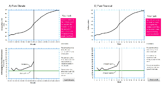
Figure 2: Screenshot highlighting the similarities and differences between the Pure Climate (a) and Pure Financial (b) tasks. Note that panel (a) depicts the same task as shown in Figure 1 but no longer shows the sketched “up” and “down” responses. In the studies we analyzed, participants were given the Pure Climate task, the Pure Financial task or a Climate/Financial task (the two tasks were never presented side by side). In the Climate/Financial task participants solved the Climate task but were given the financial context as an analogy to aid reasoning. In this condition, the inflows, outflows and stock were labelled with the climate information and the financial information alongside in parentheses (e.g., “CO2 absorption (earnings)”. The screenshot for this condition is not shown.

---

As explained in more detail in the Model section, a key advantage of the HBLMM approach is that every step of the analysis takes into account (and quantifies) the uncertainty of response classification. This quantification of uncertainty allows us to side-step the qualitative methods that are commonly used to determine response classifications (e.g., Sterman & Booth Sweeney, 2007). These standard methods necessarily involve the subjective process of deciding what kinds of responses count as representative of different types of reasoning strategies (e.g., how closely does an inflow response trajectory need to match a stock trajectory to decide that a participant has used the correlation heuristic), and there is the possibility that the classification strategy can change after data has been collected. This sort of post-hoc classification of responses is potentially problematic when counts based on these strategy classifications represent a key dependent measure in studies that examine the impact of various manipulations designed to promote better stock-flow reasoning (e.g., Dutt & Gonzalez, 2012b; Cronin, Gonzalez & Sterman, 2009, Experiment 5).

One existing approach to overcoming post-hoc qualitative assessment is to record, via computer, more precise co-ordinates of participants’ response trajectories, rather than just eyeballing pencil-and-paper sketches (e.g., Moxnes & Saysel, 2009; Newell, Kary, Moore, & Gonzalez, 2013). These precise estimates can then be used to assess the impact of manipulations by creating average response trajectories in different conditions of an experiment. However, averaging data across participants when there are discrete types of responses may also be inappropriate and can lead to non-normal distributions which may affect the conclusions of standard analyses (see Dutt & Gonzalez, 2012b, who used non-parametric tests to counter this particular problem). Outside of the assumptions of statistical tests, averaging data in a context where our theories of behavior predict that some (but not all) participants will follow a heuristic fails to address what is often a key research question: how do experimental manipulations affect the prevalence of heuristic use?

Our novel HBLMM approach provides a method for securing the best of both worlds: all of the data generated by every individual in an experiment is included in the analysis, and the principled quantification of classification-uncertainty allows for group-level conclusions regarding the impact of different experimental manipulations. This allows for a more fine-grained examination of the effects on stock-flow understanding of a potentially important manipulation – familiarity with the context in which the stock-flow problems are presented (e.g., Brunstein, Gonzalez & Kanter, 2010). Our approach builds on previous work where HBLMM approaches have proved useful in evaluating how changes in instructions and task structure affect the use of heuristics in multi-attribute choice (e.g., van Ravenzwaaij, Moore, Lee & Newell, 2014) and base rate neglect (e.g., Hawkins, Hayes, Donkin, Pasqualino & Newell, 2015).

Several recent papers have examined the effect of using more familiar stock-flow contexts in attempts to improve understanding — and communicate the urgency — of the CO₂ accumulation problem (Dutt & Gonzalez, 2012b; Dutt & Gonzalez, 2013; Gonzalez & Wong, 2012; Guy, Kashima, Walker & O’Neill, 2013; Moxnes & Saysel, 2009). Various research groups have used contexts such as the bathtub analogy (introduced earlier), balloons with two-openings, and inner-tubes surrounding the planet, with varying degrees of success. Here we build on recent work by Newell et al. (2013) and Newell, Kary, Moore and Gonzalez (2016) that used a financial debt context. Specifically, Newell et al. (2013) found that participants given a more familiar financial debt problem in a stock-flow drawing task made fewer responses that were consistent with a correlation heuristic than those given a structurally identical CO₂ accumulation problem (see Figure 2 for examples of the tasks and an explanation of the similarities and differences between them; see Appendix A for specific experimental instructions). Moreover, participants who were given the CO₂ accumulation problem but invited to think about the flows and stocks in terms of financial debt (a type of analogy) showed fewer correlation heuristic responses than those given the CO₂ accumulation task alone (Newell et al., 2013). Since Newell et al. (2013) reported a subset of the data we present here (studies 2–4 in Table 1), we expected to find the same pattern of effects over the full set of studies we report, now using our improved method of analysis instead of the averaging approach that they applied. The General Discussion reviews this evidence of an effect of familiar contexts on solving and understanding the CO₂ accumulation problem and examines the implications for theory development.

1.2  Case Study

To demonstrate the benefits of HBLMM, we use a dataset from a computer-based version of the stock-flow drawing task based on Sterman and Booth Sweeney’s (2007) hand-drawn task. Our version of the task required participants to undertake a single trial where they plotted, on a computer interface, an inflow line relative to a fixed outflow line, so that the flows were consistent with the provided depiction of stock (see Method for details).

1.2.1  The Model

The existing literature has focused on responses that either exhibited correlational reasoning or were accurate (e.g., Booth Sweeney & Sterman, 2000; Gonzalez et al., 2009; Sterman & Booth Sweeney, 2007). Thus we assumed a priori that there would be two basic response classes in the stock flow drawing task: participants who complete the emissions / amount spent lines in the lower panels of Figure 2a and 2b, respectively, by following an upward trajectory (“Up responders”), and those who indicate a downward trajectory (“Down responders”). However, in previous studies (Booth Sweeney & Sterman, 2000; Gonzalez et al., 2009; Sterman & Booth Sweeney, 2007), some participants did not fit well in either category. Thus, we also included a third class (“Other”) to capture these participants. As specified below, we had to define two rules for the “Other” class, but we subsume them in one class because the experimental manipulations focused on those who respond downwards or upwards.¹

---

Table 1: Summary of the Studies and conditions used in the analyses.

Study	Condition#	Context	N
1	1	Pure Climate	25
	2	Pure Climate	25
2	1	Pure Financial	25
3	1	Pure Climate	25
4	1	Climate/Financial	25
5	1	Pure Climate	26
	2	Climate/Financial	26
6	1	Pure Financial	25
Note: To simplify the modeling, some conditions from Study 1 and 6 were excluded from the analysis. See Appendix A for details of all conditions.

---

We use the more generic “Up” and “Down” responder labels rather than “correlation heuristic” and “correct”, respectively, because the mapping of trajectories to discrete strategy use is not one-to-one. Indeed, an advantage of our approach is the ability to quantify the uncertainty surrounding the allocation of participants to different response classes. Nonetheless, it is still the case that Up responders are more likely to be following a strategy akin to correlation-heuristic use, while Down responders are more likely to be using a qualitatively correct strategy (i.e. recognizing that some decrease in inflow is necessary to stabilize the system). We then used Bayesian hypothesis tests (Morey, Romeijn & Rouder, 2009) to determine whether the proportion of the different types of responders was the same or different across contexts (Pure Climate, Pure Financial, Climate/Financial). Our particular focus is on Up responders because this type of erroneous response pattern has received the most interest in the literature (e.g., Cronin et al., 2009).

1.2.2  Studies Overview

We conducted 6 studies over 2 years using UNSW undergraduate Psychology students. Each of these studies involved versions of stock-flow problems instantiated in the CO₂ and/or financial context, similar to the examples shown in Figure 2. For the purpose of illustrating the benefits of the HBLMM approach, we combined data from all 6 studies.

Table 1 contains the designs of each of the studies, with the order in which the studies were conducted preserved (See Appendix A for further details of each study). For the conditions coded as in a Pure Climate context, the task only included information about CO₂ accumulation – i.e. emissions, absorptions and atmospheric CO₂ (see Figure 2a; Pure Climate). For the conditions coded as in a Pure Financial context, the task included only information about financial debt accumulation – i.e. spending, earnings and total debt (see Figure 2b; Pure Financial). For the conditions coded as in a Climate/Financial context, the primary task that participants had to solve was the CO₂ accumulation one, but participants in these conditions were invited to think about the CO₂ task as analogous to accumulation of financial debt (Climate/Financial). To assist with the use of this analogy, the labels of the inflows, outflows and stock on the graphs in the climate/financial conditions contained both climate and financial terms, with the analogous financial terms in brackets, e.g., “CO₂ absorption (earnings)” (this condition is not shown in Figure 2).

2  Method

2.1  Participants

We tested 202 participants (mean age = 19.48, SD = 2.81), of which 121 were female. Participants received course credit for their participation.

2.2  Procedure

Before the task, participants were given some information about climate change (or financial debt) and were told about the inflows, outflows and stock in the system associated with their experimental condition. The text in the climate conditions was modeled on that used by Sterman and Booth Sweeney (2007).

Participants in the Pure Climate and Climate/Financial conditions were presented with on-screen figures which showed a) past and future net CO₂ stocks, and b) past CO₂ inflows (i.e., emissions) and outflows (see Figure 2a for an example). Before the task started, participants completed a small practice session to make sure they understood how to read the graphs. They had to read and report three values. For the actual task, participants were required to plot the future CO₂ emissions trajectory that would achieve the given net stock of atmospheric CO₂. Participants in the Pure Financial conditions were required to plot the future inflow (spending) trajectory to achieve a depicted stock of accumulated financial debt (see Figure 2b).

Estimation of inflows was requested for each of 10 “decades” (climate) or “weeks” (financial). For each time-period participants had to adjust an on-screen slider to their desired inflow value, which was displayed numerically. Once they clicked a button labelled “next decade”, a line would be drawn connecting the emissions/spending line to the point that the slider was moved to. Participants repeated this process until they had entered all 10 values. After the participants had entered each decadal (or weekly) value, they had an opportunity to adjust their response across all decades (or weeks). Across all studies, 69.8% of participants adjusted at least one slider. For our analysis of inflow trajectory estimation, we included only the final response (after adjustment) for each time-period. (Appendix A contains specific procedural details about each study, and Appendix B presents sample instructions from Studies 2–4).

3  Results

---

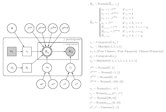
Figure 3: The graphical model used for data analysis.

---

3.1  Bayesian Model-Based Analysis

We used a hierarchical Bayesian analysis that explicitly accounts for the mixture of latent classes of responders on the trajectory estimation task. Participant data and R and JAGS code for performing the analysis have been made available on the Open Science Framework (http://osf.io/5m4y7).

As noted earlier, our a priori assumption was that there would be three basic latent categories: Up responders, Down responders, and Other responders. However, our initial model-based analyses revealed that the “Other” category contained two distinct types of responders: those producing a flat line but also those who showed an abrupt trajectory change (e.g., up and then down). Thus the Bayesian mixture model we used for our main analysis assumes that there are four populations of responders in the trajectory estimation task, and we estimate the percentage of the four types of responders in each condition.

Figure 3 shows the graphical model we used for data analysis, with standard graphical model notation. Latent and observed variables are represented with open and shaded nodes, respectively. Circular and square nodes represent continuous and discrete variables, respectively. Single and double-bordered nodes indicate stochastic and deterministic variables, respectively. Rectangular plates represent independent replications over participants and scenario conditions. To facilitate comparison across data sets we simultaneously estimated parameters for all experimental conditions (combined N = 202). This assumes that the parameters estimated for each study are informed by data from the other studies; that is, we pooled information from common conditions (Pure Climate, Pure Financial, Climate/Financial) across the six studies.

The model assumes the 10 decadal (Pure Climate and Climate/Financial) or weekly (Pure Financial) responses from each participant will be approximated by one of four linear regression models. Three of the four regression models differ only in the prior distribution placed on the regression coefficient: biased to positive values (for upward trajectories), negative values (for downward trajectories), or very close to 0 (for flat, or uncorrelated, trajectories). The fourth regression model assumed a piecewise linear function: early responses followed the upward trajectory and then, at one of the mid-to-late responses, dropped to a low value, after which responses were equivalent to the ‘flat’ model (i.e., regression coefficient very close to 0). For each participant we estimated which of the four regression models provided the best account of their 10 responses. We used these participant-level estimates to inform group-level estimates of the proportion of the four types of responders. These group-level mixture proportions – the percentage of each type of responder – are the primary focus of the inferential tests reported in the Bayesian Hypothesis Tests section.

The model assumes the ith estimate of participant j, R_ij, comes from a normal distribution with mean R_ij and standard deviation є_j. є_j is a participant-level parameter that reflects how closely participant j’s estimates approximated the regression line parameterized by R_ij. R_ij is a deterministic node whose value depends on the regression coefficients β^up, β^down,β^flat or a combination of β^up, β^drop and β^flat, which correspond to the four classes of responders; Up, Down, Other-Flat, and Other-Strategy change, respectively. Whether R_ij is generated from the Up, Down, Other-Flat or Other-Strategy change regression model is determined by z_j, a subject-level indicator variable that takes the value of 1, 2, 3 or 4 on the basis of π_k. π_k is a four-length vector that gives the probability of a responder arising from the Up, Down, Other-Flat or Other-Strategy change regression models, such that π_mk represents the probability of allocation to regression model m in scenario condition k, where ∑_m=1⁴π_mk = 1. w_j is an indicator variable that codes participant j’s scenario condition (i.e., w_j takes the value 1, 2, or 3 for Pure Climate, Pure Financial, or Climate/Financial). There is a single z_j for each participant, meaning that each participant’s data are assumed to arise from a single regression model throughout the entire experiment. Uncertainty around which regression model is correct is represented with probabilities.

---

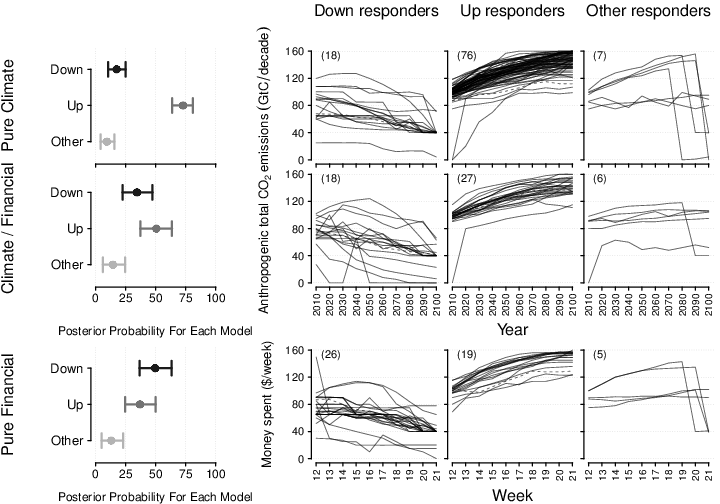
Figure 4: Estimated emissions and debt trajectories in data (upper two rows and lower row, respectively). Rows represent the Pure Climate, Climate/Financial, and Pure Financial scenario conditions, collapsed across experiments. The first column shows the Bayesian model-based estimates of the percentage of each type of responder for each grouping (i.e., posterior probability for each model), where the dot and error bars represent the median and 95% highest density interval of the posterior distribution, respectively. The rightmost three columns show the trajectories of individual participants as separate lines, classified into one of three respondent categories (“Up”, “Down”, “Other”). Solid and dashed lines show participants with, respectively, greater than 90% certainty and less than or equal to 90% certainty in the model’s estimated assignment to the respondent category. The number of participants assigned to each responder category is shown in brackets in the upper left of the panels. Note that “Other” contains participants classified as “Other-Flat” and “Other-Strategy Change.

---

For the Up, Down and Other-Flat regression models, the corresponding regression coefficient is substituted into a linear regression equation, along with the ith response position (1, 2, …, 10), and α_j, a subject-level estimate of the regression intercept. The Other-Strategy change regression model assumes a piecewise linear function which involved estimation of an additional participant-level parameter: y_j, which codes the response position (2, 3, …, 10) of the strategy change (N.B. y_j is only updated by data when z_j = 4; that is, parameter y_j carries no meaningful information for participants classified in the Up, Down, or Other-Flat regression models). The specific parameterization of the Other-Strategy change model is shown at the upper right of Figure 3. Subject-level estimates of a_j and є_j were hierarchically drawn from normal hyper-distributions with means α^µ and є^µ, and standard deviations α^σ and є^σ, respectively.

Prior settings on parameters are given on the right of Figure 3. All prior distributions were relatively vague (i.e., large dispersion) except for those relating to the regression coefficients that define the four models, for which we assumed more informative priors (small dispersion). This is because the expected pattern of responses for Up responders (those that closely adhere to the correlation heuristic) and Down responders (the correct response) are clearly prescribed for the stock-flow tasks analyzed here. Specifically, a response trajectory that follows the correlation heuristic will rise from a response of 90 at decade/week 0 to 160 by decade/week 10, implying a regression coefficient of 7 (Figure 2). Similarly, the correct response trajectory will drop from an initial response of 90 to 40 by decade/week 10, implying a regression coefficient of –5. We assumed that responses following these trajectories would be fairly precise, so we assumed a small standard deviation around these means (Figure 3). This pair of prior distributions on the regression coefficients for each responder type means that our approach classifies participants based on their proximity to the stereotyped patterns of responses in stock-flow tasks. We also allowed for minor deviations from a regression coefficient of 0 for the ‘flat’ responders, implying that a response trajectory could be classified as flat even if its slope was not strictly equal to 0.

---

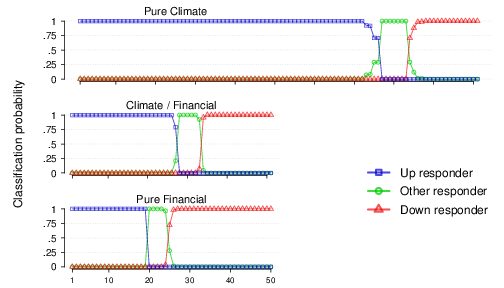
Figure 5: Classification probabilities for the response classes in each condition. The X-axis shows individual participants in order of decreasing probability of being assigned to the Up responder category from left to right. Note that there were 101 participants in the Pure Climate conditions, 51 in the Climate/Financial and 50 in the Pure Financial (see Table 1). The Y-axis is the estimated probability of classification assigned by the Bayesian analysis. The vast majority of participants are assigned either a 0 or 1 classification certainty for a particular latent response class indicating that the Bayesian mixture provides a good account of the data.

---

We performed Bayesian inference over the graphical model using Markov chain Monte Carlo (MCMC) methods in the R statistical programming environment (R Development Core Team, 2015) and Just Another Gibbs Sampler (JAGS, Plummer, 2003), using the R2jags package (Su & Yajima, 2015). We took 25,000 samples from the posterior distribution of the parameters from each of four chains with a burn-in period of 12,500 samples, for a total of 50,000 samples from the posterior distributions of the parameters. The convergence of the posterior distributions of the parameters was checked using the R statistic (Brooks & Gelman, 1998; see Supplementary Material for trace plots and marginal posterior distributions of model parameters).

3.2  Classification

The rightmost three panels of Figure 4 show the response trajectories of participants allocated to the three main respondent classes. The quality of the assignment to each category is evident in the extent that individual trajectories conform to the regression line of the category (i.e., downward in the middle left column, upward in the middle right column, and no relationship [flat] or strategy change in the rightmost column). The Bayesian analysis assigns a probability of classification to each latent class for each participant. This is shown in summary form in Figure 4: participants with greater than .9 classification certainty are shown with solid lines; the remaining participants are shown with dashed lines. Figure 5 shows the uncertainty quantification in more detail. For all but a few participants, there was strong evidence for the probability of assignment to a single category (i.e., above .9), indicating little uncertainty in the classification to latent classes, and that the Bayesian mixture suggests a good account of the data.

3.3  Bayesian Hypothesis Tests

To test whether the percentage of Up responders differed as a function of climate or financial scenarios, we conducted Bayesian hypothesis tests using the Savage-Dickey density ratio test (for tutorial, see Wagenmakers, Lodewyckx, Kuriyal & Grasman, 2010). The Savage-Dickey density ratio gives a Bayes factor indicating the weight that the evidence affords to one of two models, in particular a null hypothesis of no difference between groups versus (i.e., nested within) the alternative hypothesis that groups may differ (see Appendix C for details of the Savage-Dickey density ratio and our hypothesis tests). We use the notation BF₁₀ to refer to Bayes factors where BF₀₁ > 1 indicates support for the null hypothesis and BF₁₀ > 1 indicates support for the alternative hypothesis (i.e., we report all Bayes factors in the direction in which they provide evidence). For example, BF₁₀ = 10 indicates the data are 10 times more likely to have come from the alternative hypothesis (the two conditions have different values of the parameter) than the null hypothesis (no difference in the value of a parameter between two conditions), and BF₀₁ = 10 indicates the opposite conclusion.

In the Pure Climate scenario, a greater percentage of participants estimated an upward trajectory compared to a downward trajectory (BF₁₀ > 200,000). This is consistent with previous research, which has found that participants provide an upward inflow trajectory when the rate of CO₂ accumulation is decreasing (Dutt & Gonzalez, 2012a; Sterman & Booth Sweeney, 2007). As a measure of the size of this effect, the 95% highest density interval [HDI] of the difference in the proportion of Up and Down responders was [.396, .693]. In contrast, for both the Climate/Financial and Pure Financial scenarios the evidence was indeterminate in discriminating for or against the null hypothesis that the percentage of Up responders and Down responders was equal (BF₁₀ = 1.08, 95%  HDI  [−.081, .398], and BF₀₁ = 1.31, 95%  HDI  [−.368, .120], for the Climate/Financial and Pure Financial scenarios respectively).

The most important comparison is whether the percentage of Up relative to Down responders was different across the conditions. There was a greater percentage of Up relative to Down responders in the Pure Climate condition compared to the Pure Financial condition (BF₁₀ ≈ 4,000, 95%  HDI  [.384, .957]) and the Climate/Financial condition (BF₁₀ = 13.68, 95%  HDI  [.105, .666]). These results provide strong evidence that 1) participants can reason more appropriately when the relevant stocks and flows are presented in the more familiar context of a financial debt problem, and 2) that providing a financial analogy alongside the climate scenario reduced the proportion of inappropriate responses as compared to the climate scenario in isolation. There was indeterminate evidence regarding whether the percentage of Up vs Down responders was the same or different across the Pure Financial and Climate/Financial groups (BF₁₀ = 1.46, 95%  HDI  [−.063, .622]). This suggests that providing a financial debt analogy to assist reasoning in the climate problem might (but also might not) reduce the relative difference between Up and Down responders to the same extent as presenting the task entirely within the financial context, though this requires further investigation. There was weak evidence that the proportion of Other responders was the same across conditions: Pure Climate vs. Climate/Financial (BF₀₁ = 2.86, 95%  HDI  [−.166, .058]); Pure Climate vs. Pure Financial (BF₀₁ = 3.57, 95%  HDI  [−.149, .065]); Climate/Financial vs. Pure Financial (BF₀₁ = 3.42, 95%  HDI  [−.121, .146]).

4  General Discussion

People’s failure to reason appropriately about stock-flow systems is an enduring and intriguing theoretical puzzle that has widespread real-world implications. None more so than its potential to reinforce wait-and-see attitudes towards taking action on climate change (Newell, McDonald, Hayes & Brewer, 2014; Sterman, 2008). A commonly used assay of performance on such problems is the stock-flow drawing task. However, defining the appropriate measurement of individual performance in this task is a difficult methodological problem. We have provided a novel method that addresses this difficulty by quantifying the uncertainty in classification of individual stock-flow task responses.

Using hierarchical Bayesian latent mixture models (HBLMM) with three basic response classes, we were able to classify most participants into one class with high certainty (over 90%). Broadly consistent with previous research, we found a larger proportion of participants in the climate version of the trajectory estimation task responded with an Up trajectory relative to a Down trajectory. We also found evidence that presenting the same problem in a familiar financial context and using a financial analogy for the climate context produced fewer Up responders relative to Down responders than in the climate context alone. However, we only found indeterminate evidence for whether there was a difference in the proportion of Up relative to Down responders between the financial context and the climate/financial context. The climate/financial context may or may not improve performance on the task to the same degree that the financial context does. This comparison requires further investigation.

4.1  The benefits of HBLMM

Our use of HBLMM builds on recent successful applications in other decision-making problems such as base-rate neglect (Hawkins et al., 2015) and multi-attribute choice (van Ravenzwaaij et al., 2014). Performance in these tasks, in common with the stock-flow problem, is often attributed to the use of a heuristic, or a discrete strategy that is consistently applied by multiple individuals in an experiment (e.g., Gigerenzer & Goldstein, 1996; Tversky & Kahneman, 1974). However, it is rarely the case in any given experiment that all participants are using the same heuristic – some participants may know the solution to the problem they are faced with, or be applying another strategy (e.g., Newell, 2005). Popular responses to this analysis problem are to ignore the individual variability by averaging across all participants, or to engage in post-hoc classification of response profiles; an inherently subjective process which can lead to the drawing of “fuzzy” boundaries that are potentially problematic for some types of statistical inference. Subjectivity in response classification could be reduced by including multiple independent raters. This approach however would still produce problem cases where the raters disagree about the appropriate classification. Currently no principled method exists for resolving such disagreements beyond encouraging raters to reach a consensus or using the classification favored by a majority of raters. Researcher classification (by either single or multiple raters) also ignores classification uncertainty, or the extent to which a classified response could have been produced by a different strategy.

HBLMMs provide a more principled and more fruitful solution by acknowledging the presence of individual differences in responding—thereby incorporating all the data from all individuals—and providing an objective quantification of the uncertainty associated with different response classes. HBLMMs are, however, not a panacea for analyzing these kinds of data. A close inspection of Figure 4 reveals some examples of idiosyncratic responses that are categorized with high probability into one of the classes (e.g., the participant in the Climate/Financial condition who produced a downward response with a “triangle” mid-trajectory – middle panel of middle left column). While it may be tempting to create new classes in the model to capture these unusual responses, this raises the problem that as the number of classes increases, the probability of an individual being assigned to a given category is reduced. This is because as the number of classes increases, the difference between the classes becomes smaller, and any particular individual’s data could have been generated by more than one strategy in the model. Thus there is a trade-off between the precision of the model (or how well it captures the individual differences in the population) and its explanatory power (or how we can use the model to make theoretical advances). The point raised here is not a problem for the model per se. The problem arises because the experimental task allows for unconstrained responding, which causes a problem for any analysis approach.

In the current research, we suggest that the classes we defined are useful to developing theories of performance in stock-flow reasoning, but also differentiated enough to maintain a high level of certainty for most of our classifications (> 90% in most instances). If we chose to define our “downward trajectory” class as the actual correct response, we would have to define a very flexible rule (the correct response is nonlinear – see Figure 1) which would undermine the certainty in our classification. Yet, someone drawing an upward trajectory is qualitatively different in important ways to someone drawing a downward trajectory. This difference, which is captured by the model, allows us to advance understanding of how factors such as context familiarity affect performance on this task.

4.2  The role of context familiarity in stock-flow reasoning

The research presented here converges with Newell et al. (2016) in establishing the financial context as one which reduces the proportion of participants using correlation-like (upward trajectory) responding in comparison to a CO₂ accumulation scenario. In contrast with Newell et al. (2016), we also found a beneficial effect of presenting the financial analogy in the climate context. The reason for this inconsistency might lie in procedural differences between the tasks used in the two studies. Newell et al. (2016) used a modified version of the graph drawing task that only required participants to enter the final value of the emissions or spending trajectory (i.e., at the year 2100 or week 21 in the lower panels of Figure 2a and b, respectively) rather than plot the entire line (see Guy et al., 2013 for a similar method). Newell et al. (2016) speculated that the one-shot nature of this single-value prediction task might attenuate the beneficial effect of the financial analogy. Perhaps when participants are required to draw the line in its entirety, they have more instances (10 responses compared to 1) to reflect on the analogy and integrate it into their responses. Future research into the effects of analogy on reasoning in stock-flow problems could investigate how the task (e.g., final-value estimate vs. entire trajectory drawing) interacts with the analogy to help promote appropriate responding.

An outstanding question regarding the financial context is why it works. Does it encourage fewer people to use correlation-like responding because the context helps them better understand the structure of stock-flow systems (because the concepts of earning, spending and debt are more familiar than emissions, absorption and CO₂ accumulation), or are people simply relying on a different cognitive bias, such as valence? Newell et al. (2016) found evidence to suggest that individuals may draw a downward trajectory because they are following a valence rule such as “debt is bad, so reduce spending” rather than because they understand the relationship between the stock and flows. Thus the financial context and analogy may reinforce the idea that the world needs to reduce CO₂ emissions (as opposed to simply stopping them from rising) — a desirable outcome from a climate science communication perspective — but it does not necessarily indicate an improved understanding of how stock-flow systems work.

While it seems unlikely that any single context can lead to perfect performance on stock-flow problems, there is still scope to find a series of contexts, analogies and tasks that can be combined to help people better understand the abstract relationship between stocks and flows. Gonzalez and Wong (2012) suggest that successful analogies need to maximize both the surface and behavioral similarity of the analogy to the target problem, with behavioral similarity indicating that the analogy has the same underlying functional form as the target problem. Beyond that, we can also make the comparison between contexts even more explicit by asking participants to list the similarities and differences between the contexts (in our example, climate change and debt), which has been shown to have positive effects on analogical transfer (e.g., Gonzalez and Wong, 2012; Smith & Gentner, 2012).

4.3  Limitations and Future Research

One potential limitation of the current work is that the studies were conducted sequentially over time and as a result participants were not allocated randomly to the contexts analyzed here (with the exception of data from study 5 – see Appendix A). While we acknowledge that a randomized experiment is the gold standard of empirical research, we do not think that the lack of random allocation is a serious problem in the current analysis. The population remained approximately constant, as all participants were students of the same university. Each context also featured data from more than one study (conducted at different times), which reduces the chances that all data in a context reflect a biased sample rather than a genuine effect.

There were also some small differences between the studies that were not simply due to changes in instructions. For example, some conditions included in the model came from factorial designs or featured additional tasks (e.g. Study 1). In future, the HBLMM could be extended to take such study differences into account by allowing the parameters of the model to vary across studies. We decided only to allow parameters to vary across individuals in the current work in order to provide a relatively simple demonstration of the potential of HBLMMs for the analysis of stock-flow reasoning data. Without having strong reasons for expecting theoretically important effects to be driven by study differences, we think that our admittedly more coarse level of analysis provides a good compromise.

The HBLMM approach we have outlined in this paper could also be used to analyze other variants of stock-flow tasks. For example, researchers have used a stock-flow drawing task in which participants had to draw the accumulating stock rather than the inflow (Cronin et al., 2009). In the stock drawing task, a typical correlation heuristic response would be to draw a stock line that mimics the inflow line; it would be simple to apply our approach to characterizing responses in this version of the task. HBLMMs can also be applied to one-shot responses such as those found in the “department store” task (Sterman, 2002) or the climate task used by Newell et al. (2016). In the department store task, participants are presented with a graph tracking the inflow and outflow of customers in a store over a certain time period and are asked when the most and fewest customers are in the store. This task also involves a continuous dependent variable, but there is a correct response and a typical correlation heuristic response, likely leading to a bimodal distribution of responses. Hawkins et al. (2015) presented a HBLMM for one-shot responses in the context of a base-rate neglect problem also characterized by bimodal distributions of responses, so a similar approach to theirs could be applied.

Regardless of the task that researchers use to measure stock-flow reasoning, we need an appropriate method of inferring the impact of any manipulation on performance. HBLMMs provide such a principled inferential method to classifying responses in this important class of reasoning problems.

References

Appendix A

In this appendix, we provide brief summaries of the original studies. All studies featured a Pure Climate condition, a Pure Financial condition or a Climate/Financial condition as specified in the main text. In addition, some studies contained further manipulations, with those conditions removed from the HBLMM. For each study, we specify the conditions that were used in the HBLMM, the total N for each study and any additional manipulations that were not included in the main text. For further information on the protocols of the studies, please contact the corresponding author.

Study 1

Conditions in Model: Pure Climate (n = 50).
N: 100 participants (70 female)
Additional manipulations: This study featured a 2 x 2 factorial design, with participants randomly allocated to conditions. The first factor was whether participants were required to draw the inflow of accumulating stock of CO₂. The second factor was an analogy manipulation based on Gick and Holyoak (1980). Participants were given a relevant or irrelevant story before completing the Pure Climate condition, were provided with a hint about the story, and then completed the Pure Climate condition again. The relevant story invited participants to think about how inflatable jumping castles are inflated and kept “solid” enough to jump on. This involved some descriptions of in-flows and out-flows and stock of air. The irrelevant story asked participants to think about a logic problem (a variation on a Knights and Knaves problem) — there was no mention of stocks and flows. Using the non-Bayesian RMSD analysis method described in Newell et al. (2013), we found no statistically significant effect of analogy on any aspect of responding, so in the analysis reported in the body of the paper we included data from the two conditions in which participants drew the inflow.

Study 2

Conditions in Model: Pure Financial (n = 25).
N: 25 participants (12 female)
Additional manipulations: None.

Study 3

Conditions in Model: Pure Climate (n = 25).
N: 25 participants (15 female)
Additional manipulations: None.

Study 4

Conditions in Model: Climate/Financial (n = 25)
N: 25 participants (17 female).
Additional manipulations: None.

Study 5

Conditions in Model: Pure Climate (n = 26) and Climate/Financial (n = 26).
N: 52 participants (27 female)
Additional manipulations: In this study, participants first completed a Pure Climate condition. They then completed either the Climate/Financial condition or repeated the Pure Climate condition, with participants randomly allocated to conditions. We only used the responses from the second attempt (Climate/Financial or Pure Climate) in the model.²

This study also involved a modification to the graphs presented to participants. Instead of the formatting displayed in Figure 1, participants saw a stock graph that had a larger range on the y-axis (from 600 to 1000 GtC). This meant that there was some additional whitespace between the stock line and top of the graph in an attempt to aid the visualization of stabilization in the stock graph.

Study 6

Conditions in Model: Pure Financial (n = 25)
N: 101 participants (61 female)
Additional manipulations: This study also included a 2 x 2 factorial design, with participants randomly allocated to conditions. The first factor was whether participants drew the inflow or stock in a Pure Financial condition. The second factor was the shape of the stock-flow function. We only included the condition that involved drawing the inflow and had the same function as the other studies.

Appendix B

This appendix contains samples of the instructions used in Studies 2–4. For the Pure Climate and Pure Financial contexts, participants read the instructions specified below. For the Climate/Financial context, the text below was presented after participants had read the instructions for the Pure Climate context.

Sample instructions for the Pure Climate context:

Consider the issue of global warming. In 2001, the Intergovernmental Panel on Climate Change (IPCC), a scientific panel organized by the United Nations, concluded that carbon dioxide (CO₂) and other greenhouse gas emissions were contributing to global warming. The panel stated that “most of the warming observed over the last 50 years is attributable to human activities.”

The amount of CO₂ in the atmosphere is affected by natural processes and human activity. Anthropogenic CO₂ emissions (emissions resulting from human activity, including combustion of fossil fuels and changes in land use, especially deforestation), have been growing since the start of the industrial revolution. Natural processes gradually absorb CO₂ from the atmosphere (for example, as it is used by plant life and dissolves in the ocean). The top graph shows an atmospheric CO₂ scenario, in which the amount of atmospheric CO2 rises from an initial value of just over 600 gigatonnes of carbon (GtC) but then over a period of 210 years stabilises (does not increase any more) at 945 GtC.

On the bottom graph the green line shows how much CO₂ is absorbed per decade – it remains constant at 40GtC – the black line shows how much CO₂ is emitted per decade – it rises up to the year 2000.

Your task will be to correctly extend the line (on the lower graph) representing “CO₂ emissions” in relation to the “CO₂ absorption” line, from the year 2010 to 2100, so that the bottom graph depicts the atmospheric CO₂ scenario shown in the top graph.

Sample instructions for the Pure Financial context:

The amount of money in your bank account is determined by how much you earn and how much you spend.

Imagine that you have gotten yourself into debt, but you are now trying to prevent the debt from getting any bigger. For example, the top graph below shows how your debt might increase from an initial value of just over $600 but then over a period of 21 weeks stabilises (does not increase any more) at $945. There is no interest charged on the debt you owe.

On the bottom graph the green line shows how much you earn per week – it remains constant at $40 – the black line shows how much you spend per week – it rises up to week 11.

Your task will be to correctly extend the line (on the lower graph) representing “dollars spent”, from weeks 12 to 21, given the debt shown in the top graph.

For each week after Week 10 you will be presented with a slider, which you need to adjust to show the number of dollars spent that week. Once you adjust the amount and click “next week” you will not be able to change your response.

Additional instructions for the Climate/Financial context:

You might like to think of controlling the level of CO₂ in the atmosphere as similar to controlling your personal finances. If you spend more than you earn you get into debt, and if you keep spending more than you earn that debt grows.

The amount of CO₂ in the atmosphere is like our current ‘debt’ level and just as you would not want your debt to get bigger, we don’t want atmospheric CO₂ levels to keep rising. The top graph shows a situation in which this goal is achieved (i.e. CO₂ levels stop rising) by 2100.

You can think of the CO₂ emissions line on the bottom graph as the money you spend and the absorption line as the money you earn. In order to stabilise CO₂ levels (or in other words stop your debt increasing) what would you need to do?

Try to use this idea to extend correctly the line (on the lower graph) representing “CO₂ emissions”, from the year 2010 to 2100, given the amount of atmospheric CO₂ shown in the top graph.

Appendix C

In this appendix we provide a detailed explanation of the Savage-Dickey density ratio test used in the main text to conduct hypothesis tests. Our hypothesis tests examined whether there was a difference in the number of particular types of responders within and between conditions. For example, in one test we examined whether there was a difference in the percentage of Up and Down responders in the Pure Climate condition. In another test, we examined whether the difference in the proportion of Up and Down responders was different between the Pure Climate and Pure Financial conditions. Our tests thus focused on the π parameter from our Bayesian mixture model, which refers to the probability of an emissions/debt trajectory arising from the “Up”, “Down”, “Other-Flat”, or “Other-Strategy change” regression models. To be precise, π_k is a four-length vector with elements that correspond to the four latent populations, such that π_mk represents the probability of assignment to regression model m∈ {Up, Down, Other-Flat, Other-Strategy change} in scenario condition k where and ∑_m=1⁴π_mk = 1.

Our hypothesis tests were comprised of pairwise dependent comparisons between pairs of posterior distributions of π. In a similar vein to the paired samples t-test, we take the difference between the posterior distributions of elements of π and test whether the difference is equal to zero (null hypothesis) or different to zero (alternative).

Our analyses had two broad aims. Firstly, in each condition we tested whether there was a different proportion of participants responding in a manner consistent with the correlation heuristic (Up) or trending toward the correct response (Down). We denote this difference between two elements of the posterior distribution of π as δ; for example, δ_climate=π_up,climate − π_down,climate. Comparison of the respective elements from Figure 4 of the main text (upper and middle dots of the upper left panel) suggests the posterior density of δ_climate is shifted away from 0 in this example, indicating a difference in the proportion of the two responder types for this condition. Secondly, and our primary focus, we tested whether the difference in the proportion of Up and Down responders differed across scenarios, implicating a role of framing on comprehension of the trajectory estimation task; for example, whether the posterior density of δ_climate − δ_financial is centered at 0. The Savage-Dickey density ratio uses the prior and posterior distributions of δ to compare two models that correspond to conventional two-tailed hypothesis tests: the null hypothesis that there is no difference in the posterior distributions of π_mk between two conditions, H₀:δ=0, and the alternative hypothesis of a difference between the two posterior distributions, H₁:δ ≠ 0.

We used uninformative Dirichlet distributions as prior distributions on π_k. The Dirichlet distribution is the multivariate generalization of the beta distribution and is the conjugate prior of the categorical distribution. The prior distribution for the two types of differences – that is, differences in the proportion of Up and Down responders within and between conditions – differ slightly in form. We obtained these prior distributions through sampling in our model-based analysis, and use these as the prior distribution for H₀.

The Savage-Dickey density ratio is given as the ratio of the density of the prior to posterior distributions at the point value of relevance to the null hypothesis (i.e., δ=0). For example, the Bayes factor for the difference in the proportion of Up and Down responders between the Pure Climate Climate/Financial scenarios is approximately 1/.0731 ≈ 13.68). This ratio is a Bayes factor (BF) that gives the relative odds that the data were generated by the alternative hypothesis compared to the null hypothesis, where BF₁₀ > 1 indicates support for H₁ and BF₀₁ > 1 supports H₀. Following Lee and Wagenmakers (2013), we used the logspline non-parametric density estimator from the polspline package in R (Kooperberg, 2015) to obtain prior and posterior density estimates for hypothesis testing.

*

School of Psychology, University of New South Wales, Sydney 2052, Australia. Email: a.kary@unsw.edu.au.

#

School of Psychology, University of New South Wales and School of Psychology, University of Newcastle.

$

School of Psychology, University of New South Wales.

This work was supported by an Australian Research Council Future Fellowship (FT110100151) to the fourth author, Australian Research Council Linkage Project (LP120100224) and Discovery Project (DP120100266) Grants to the third and fourth authors, and an Australian Research Council Discovery Early Career Researcher Award (DE170100177) to the second author. We thank Chris Moore and Coty Gonzalez for their contributions to this project. We also thank Michael Lee, Jeffrey Chrabaszcz and Daniel Heck for their helpful comments.

Copyright: © 2017. The authors license this article under the terms of the Creative Commons Attribution 3.0 License.

1

One can think of responses allocated to this extra class in the same way that one thinks of chance responders as a model contaminant in other tasks. Hence to make accurate inferences about the proportion of responders using an “Up” or “Down” data generating strategy, we need to remove responders that are not using either strategy. Instead of using exclusion criteria to remove such responders from our analysis completely, we instead create the “Other” class and use the same model to probabilistically classify contaminant responders as we do to classify responders to our target categories. In this case, we have defined the “Other” class to capture contaminants in a post-hoc fashion, given that it was difficult to predict a priori the kind of responses that would not fit into either target category, but ideally contaminant strategies should be defined before collecting data. Nonetheless, an extra benefit of HBLMMs is that they can also help us address the “fuzzy” boundary problem associated with exclusion criteria.

2

This study also included some measures related to climate change attitudes after the drawing task, but these are not considered relevant to the primary research question of this article.

This document was translated from L^AT_EX by H^EV^EA.