We demonstrate that the desirability bias, the elevation of the
estimated likelihood of a preferred event, can be due in part to
the desire for consistency between the preference for the favored
event and its predicted likelihood. An experiment uses a
participant’s favorite team in Major League Baseball games and a
recently devised method for priming the consistency goal. When
preference is the first response, priming cognitive consistency
moves prediction toward greater agreement with that preference,
thereby increasing the desirability bias. In contrast, when
prediction is the first response, priming cognitive consistency
facilitates greater agreement with the factual information for each
game. This increases the accuracy of the prediction and reduces the
desirability bias.
The desirability bias (DB) is the upward distortion of the estimated
likelihood of a desired event and, less frequently, the downward
distortion of an undesired event. Its costs can be substantial: for
instance, failure to protect against possible negative events like
unemployment and unsupportable debt (Williams, 2009; see also
Shepperd, Waters, Weinstein & Klein, 2015) and decisions to change
career direction when college grades fall short of biased estimates
(Serra & DeMarree 2016). Doubts about the validity of the many reports
of its occurrence (Krizan & Windschitl, 2007) have been eased by
demonstrations of its presence when the desire for one outcome is
randomly assigned (Windschitl, Scherer, Smith & Rose, 2013) and when
a reward as large as $50 is offered for unbiased accuracy (Massey,
Simmons & Amor, 2011; Simmons & Massey, 2012; see also Muren, 2012).
Given the existence of the DB, a natural next question is what causes
it. Krizan and Windschitl’s (2007) thorough analysis revealed nine
mechanisms that could produce a DB. The objective of the present work
is to test the goal of cognitive consistency as a tenth cause. In
addition, cognitive consistency is a component of three of Krizan and
Windschitl’s nine mechanisms.
1.1 Cognitive consistency
Cognitive consistency (CC) is the consistency among related
beliefs. Its history in psychology extends back at least to the work
on cognitive dissonance in the 1960s. In the years since, CC has
continued to be studied, sometimes under different names (e.g.,
balance and coherence) and variously conceptualized as a goal, a
procedural mindset, and a fundamental property of belief systems
(Chaxel & Russo, 2015; Gawronski & Strack, 2012). In the present
work, CC is viewed as the goal of enhancing the agreement among
related beliefs. (We use the term “belief” broadly, to include
preferences.)
The DB is defined in terms of two closely related beliefs, the desire
or preference for an event (the Preference) and the estimated or
predicted likelihood of that same event (the Prediction). Our claim is
that the DB can be driven, in part, by the goal of making the beliefs
of Preference and Prediction more consistent and, more specifically,
by altering Prediction to become more consistent with Preference. If
CC can do this, then a tenth, conceptually distinct mechanism can join
Krizan and Windschitl’s (2007) list. CC also forms a part of three
members of this list, viz., valence priming and negativity bias in the
information-search category and differential scrutiny in the
information-evaluation category. For instance, valenced priming “is
based on the enhanced activation of positively valenced knowledge
(knowledge consistent with desired outcome)” (p. 108).
One challenge for a CC-based explanation of the DB is the absence of
directionality. Because the DB is only the unidirectional movement of
Prediction to better accord with Preference, a consistency-satisfying
nondirectional agreement between Preference and Prediction cannot, by
itself, account for the DB. Any explanation that relies on CC must
also include a source of direction and specifically the movement of
Prediction to better accord with Preference. For instance, each of the
three Krizan and Windschitl (2007) mechanisms mentioned above provides
that necessary direction. In valence priming, it is the differential
activation only of “knowledge consistent with desired outcome”. Note
that the opposite directional change, where Preference is altered
toward greater agreement with Prediction, is entirely
possible. Indeed, it is sufficiently common in political elections to
merit its own label, the bandwagon effect (e.g., Mehrabian, 1998;
Morwitz & Pluzinski, 1996), and to make familiar the saying that
everyone likes a winner (e.g., Ashworth, Geys & Heyndels,
2006). Elster (1983) has also called it a “sour grapes” effect when
it works to reduce preferences for outcomes deemed unlikely.
1.2 Dominance of preference over prediction
The source of direction that must accompany the nondirectional CC in
order to explain the DB is provided by the dominance of the Preference
belief. This dominance occurs for two reasons. First, Preference is
usually the stronger, more stable belief. In a sports contest, which
is the experimental setting of the present work, the Preference for a
favorite team is usually rooted in past experience, often originating
in youth, and reinforced over time (e.g., Cialdini et al., 1976). Such
a Preference inherently resists alteration. Second, of the two
beliefs, Preference is more independent of contextual factors. In
contrast, Prediction, the estimated likelihood of a favorite team’s
victory in a particular contest, depends on such factors as the
strength of the opponent, the actual players (e.g., which players are
currently injured), where the game is being played (home or away),
etc. Thus, the greater context-dependence of Prediction leaves it more
exposed to influence, while Preference remains largely independent of
the same considerations. The import of the relative strength of
Preference over Prediction is that any movement toward greater
agreement between the two means that Prediction is much more likely to
do the moving, at least in a sports context.
1.3 Response order: Preference first or prediction first
Should we expect the order of the Preference and Prediction responses
to matter, especially under the pressure of an activated goal of CC?
Suppose that an experimental paradigm asks, “Which team would you like
to win?” followed by something like, “Completely ignoring your
personal preference, which team do you believe will win?” We suggest
that the combination of collecting the Preference response first and
activating the consistency goal might enhance the role of this already
dominant belief, leading to increased DB. That is, when the first
response is Preference, this belief is activated and, combined with a
previously activated consistency goal, drives the subsequent
Prediction toward greater agreement with it, hence a greater DB.
However, what should be expected if the response order is reversed
(and the consistency goal is activated), so that participants are
first required to provide the Prediction? We proffer three possible
processes: (a) the continued dominance of Preference, (b) consistency
with the facts, and (c) a bandwagon effect, in which the Preference
changes to fit the Prediction. The different empirical impacts on
Prediction, the DB, and strength of preference expected from these
alternative processes enable us to distinguish them.
Preference still dominates. The first mechanism is the
unchanged dominance of Preference. The strength and stability of
Preference, combined with the context-dependence of Prediction,
suggest that the consistency goal will produce the same increase in
the DB whether Prediction or Preference is the initial response. Order
may matter even less when participants know that they will have to
provide both responses, one right after the other, as they do in most
studies of the DB, including ours. This mechanism would leave
Preference dominant and, when CC is primed, yield the same increase in
the DB as when Preference is the first response.
Consistency with facts. The second mechanism relies on
consistency with the facts of the particular baseball game. Consider
the stimulus that participants face before their first response, that
is, immediately before having to make their Prediction. Because they
start by reading the names of the two teams and various facts
pertinent to the contest between them, participants can achieve the
consistency goal by making their estimates of Prediction accord with
these game-specific facts (before confronting the Preference
question). If CC drives facts-Prediction agreement rather than
Prediction-Preference agreement, the result should be a more
fact-based, accurate estimate of Prediction and, therefore, a
reduction in the DB.
A bandwagon effect. The third process is a sports version of
the bandwagon effect in politics in which the candidate most likely to
win draws elevated preference ratings. If a bandwagon effect occurs,
not only does activating the CC goal not move Prediction toward
Preference, but Preference changes to better accord with the
Prediction that has just been made. This process predicts that change
in the Prediction of a team’s success (e.g., as the result of
increased consistency with facts) is associated with a corresponding
change in Preference for that team. We used a Strength-of-Preference
measure to asses such changes.
We do not a priori favor any of these three processes for achieving CC
when Prediction is the first response and CC is activated. Instead, we
let the data reveal whether the DB increases (indicating the continued
dominance of Preference) or decreases (indicating greater consistency
with facts) and, in addition, whether Strength of Preference changes
in parallel with any change in Prediction (indicating a bandwagon
effect).
Note that the above predictions for the order of the Preference and
Prediction responses hold under that assumption of an activated goal
of CC. The main focus of this work is whether CC can play a role in
the DB and, if so, what that role is. If such a role is found, then
whether CC affects the DB in ordinary circumstances should depend on
the ambient activation level of this goal. However, future work to
identify the naturally occurring activation levels of the consistency
goal only makes sense once the experimental activation of this goal
has first been demonstrated to have an effect. Thus, the following
study focuses only on differences between the activated and control
conditions for the two response orders.
1.4 A sports context
To test the claim that priming CC will increase the DB when Preference
is the first response and to reveal the process when Prediction is the
first response, we chose the context of sports games, specifically
Major League Baseball. This setting has been used in other empirical
investigations of the DB (e.g., Babad, 1987; Simmons, Nelson, Galak &
Frederick, 2011). This context carries at least two material
advantages. First, it should provide an identifiable Preference in the
form a participant’s favorite team (Massey, Simmons & Armor,
2011). Indeed, we required participants to be baseball fans and to
have a favorite team. The existence of such a favorite provides a
solid indicator of group identification, which has been shown to
predict the DB in past studies (Babad, 1987; Dolan & Holbrook, 2001;
Hirt, Zillmann, Erickson & Kennedy, 1992; Markman & Hirt, 2002;
Price, 2000).
A second benefit of the sports context is its potential to complete
the only other test of the power of the consistency goal to increase
the DB. Chaxel, Russo and Wiggins (2016) demonstrated how activating
the goal of CC could increase the DB in the context of the Academy
Awards. They showed that the number of matches between the preferred
and predicted winners of the six major awards rose from a baseline of
2.34 in the control condition to 3.05 for consistency-primed
participants. However, because Chaxel et al. had no way to measure the
number of matches with zero DB, they could not claim the presence of
any DB in the control/unprimed condition. (Maybe 2.34 matches could
have been achieved merely by choosing the predictions of credible film
critics, thereby ignoring all personal preferences for award winners.)
Instead, Chaxel et al. could show only that priming the consistency
goal increased the DB relative to the control group. The measure
necessary to compute the baseline DB is essentially an authoritative
prediction of the likelihood for each award, something problematic for
unique events like Academy Awards. However, these predictions are
available for Major League Baseball games in the form of the unbiased
probability of each team’s victory. Therefore, in the present study we
should be able both to assess the baseline magnitude of the DB
relative to an unbiased standard (which Chaxel et al. could not) and
also to compare that baseline to the corresponding effect when CC is
primed.
To the above two advantages of the baseball context can be added a
third. A numerical magnitude of the DB for every individual prediction
enables a stricter test of the influence of CC. Not only should the
consistency goal drive Prediction toward greater agreement with
Preference (at least when Preference is the first response), but the
strength of preference for the favorite team should yield a
continuously elevated Prediction. Because this increase in Prediction
is equivalent to more DB, greater desire as assessed by a greater
strength of preference should monotonically produce a larger DB.
2 Method
2.1 Participants
Based on pilot data, we initially desired 800 participants. We were
able to recruit 741 Mechanical Turk workers: age (M = 33.57, SD =
15.7); gender (69.6% male); English as the first language (98.9%);
American citizens (100%). All were required to have a favorite Major
League Baseball team and to demonstrate sufficient baseball knowledge.
To ensure that participants were genuinely knowledgeable about Major
League Baseball, we constructed a knowledge test comprised of ten
4-alternative multiple choice questions.1 Over all participants, the mean number correct was
5.62. However, because some individuals might have falsely stated
their status as baseball fans or overestimated their baseball
knowledge, we eliminated the 23 lowest-scoring participants, those who
answered no more than one question correctly.
Participants were initially asked to identify their favorite baseball
team. However, when presented with the game involving that team, 9
participants preferred the opponent. We judged these 9 not to have had
a favorite team and disqualified them. This left a final sample of
708.
2.2 Materials and procedure
Games. The data were collected in three waves of games during
August and September 2014. Each participant responded to 8 Major
League Baseball games, one of which always involved the favorite
team. Because this game was the only one that assured a clear
preference, only it qualified for testing our predictions. The other 7
games served as distractors so that participants would be less likely
to detect our focus on the one game involving their favorite
team. Note that we chose only days when all 30 MLB teams played (15
teams in each league), so there were always 7 American League games, 7
National League games, and one inter-league game that involved a team
from each league. This enabled all 8 games to be played by teams from
the same league as the favorite, with the exception of the single
inter-league game that had to appear in both sets of 8 games.
Information for each game matched that commonly given in sports news:
the two teams and their win-loss records, the starting pitchers with
their respective win-loss records and earned run averages, venue
(i.e., the host team), and start time (i.e., a day game or a night
game). The two-part Preference response asked, “Which team would you
like to see win? How much would you say that you care about who wins
this game (strength of preference scale, 0 to 100)?” To make clear in
the data analysis that preference was assessed on a continuous scale
and was not just the identification of one competing team as the
preferred team, we use the label Strength of Preference for this
variable. The two-part Prediction response was, “Please predict the
winner to the best of your ability and knowledge. This is the team
that you believe will win, regardless of whether you want them to win
or whether you believe that they should win. Express your confidence
in the predicted winner (probability scale, 50 to 100).” As with
Strength of Preference, to clearly signal that prediction was measured
continuously, we label it Predicted Likelihood.
For all games, authoritative estimates of the probability of each
team’s winning were created by averaging the predictions of the four
models provided by http://TeamRankings.com. The proportion of game winners
correctly predicted by these models was .56 over all games during the
2014 Major League baseball season. This value might reasonably be
interpreted as an indication of how difficult it is to predict the
winner of a typical Major League Baseball game. For completeness, we
note that the proportion of correct game winners for the 45 games
actually used in our study was .58.
Table 1: The complete design, with the leftmost two columns showing
the consistency-priming conditions and the two rightmost two columns
showing the matched non-priming (control) conditions included to
test for an effect of serial position on the DB. The numbers of
participants assigned to each of the four conditions/columns are
given below each one. The counts in the eight cells indicate the
numbers of participants who encountered the game involving their
favorite team before or after the consistency-priming or matched
non-priming task. Note that all participants in the two leftmost
columns saw their first four games (possibly including the game that
involved their favorite team) before the priming manipulation.
Those games are labeled unprimed/control and were considered control
games in our analyses. As a result, about three times as many
participants considered the game involving their favorite team while
in the unprimed or control condition as in the consistency-primed
condition.
Serial position
Preference first
Prediction first
Preference first
Prediction first
1–4
Unprimed control (n=82)
Unprimed control (n=96)
Control (n=91)
Control (n=80)
Priming consistency
Matched non-priming
5–8
Primed (n=87)
Primed (n=78)
Control (n=98)
Control (n=96)
Total n
169
174
189
176
Consistency prime. Halfway through the complete set of 8
games, all participants were told “There will be 4 more games for you
to give us your opinions about. However, we want them to be
independent of any carry-over from your baseball thoughts during the
first 4 games. So we have inserted two mind-clearing tasks.” The first
of these two tasks activated the goal of CC. It was described as
“critical reasoning”, with instructions that began, “On the next page
you will get a double challenge: to explain a conflicting set of
facts, and to do so in only 3 minutes. Please work for the full 3
minutes. Provide explanations that go beyond the ‘obvious’ answer.”
(See Supplemental
Materials for complete instructions and stimuli.) There were two
versions of the “critical reasoning” task, one designed to prime the
goal of CC, the other a matching control. For those participants
receiving the priming manipulation, the goal of cognitive consistency
was activated by asking participants to resolve a difficult conundrum,
“Why do most people today strongly reject prejudiced social beliefs
from a hundred years ago on intrinsic grounds, even though there is
basically no intrinsic difference between people today and people from
the beginning of the last century?“2 Those participants assigned to the
control version of the “critical reasoning” task responded to a much
easier version of the above question, “Why do most people today
strongly reject prejudiced social beliefs from a hundred years ago?”
The change from the conundrum to its modified version has been shown
to create substantial differences in the activation of the consistency
goal (Chaxel et al. 2016).
The second “mind-clearing task” inserted a delay that further
activated the consistency goal by not permitting progress toward
achieving it (Chaxel & Russo, 2015). This is a standard tactic that
increases a primed goal’s activation level by frustrating its
achievement for a brief period (Fishbach & Ferguson, 2007; Forster,
Lieberman & Friedman, 2007). To accomplish this in our experimental
procedure, participants had to spend another 3 minutes reading a
300-word article on the evolution of the horse
(http://en.wikipedia.org/wiki/Evolution_of_the_horse). They were
warned that later they would be tested for knowledge drawn from this
article. Note that all participants completed both “mind-clearing”
tasks, spending the same total time (3 minutes) on each one. The only
difference was having to work on the conundrum (the primed group) or
its easier version (the control group).
Design. The main design consisted of two factors that were
crossed: the priming of the consistency goal (primed versus
unprimed/control) and response order (Preference-first or
Prediction-first). The rest of the design involved the serial position
of the 8 games: an initial set of 4 and a final set of 4 that were
always separated by the activation of the consistency goal (or its
corresponding control task). The structure of this design is portrayed
in Table 1, with consistency priming in the two leftmost columns and
matched non-priming in the two rightmost columns. All participants
were randomly assigned to one of these four columns.3
On each of the three days of data collection, the 8 games in each
league were randomly partitioned into the two sets of 4. These, in
turn, were randomly assigned to be either the initial or final set of
4 games. For each set of 4, an order of presentation was chosen
randomly and reversed for half of the participants. Note that in the
two primed conditions (the two leftmost columns in Table 1), the
initial 4 games before priming could serve as controls for the final 4
games post-priming, but only if their value as controls was not
invalidated by an effect of serial position due to learning, fatigue,
or boredom over the 8 games. However, analyses revealed that the DB
did not differ reliably across serial position, the two sets of games
or the two orders of presentation of these sets. Thus, neither serial
position nor these counterbalancing factors is discussed further.
The only substantive result of the test for serial position was to
provide three times as many control games as primed games. In our
primary analyses below, we focus on games that involved participants’
favorite teams. For about half of the participants assigned to the
consistency-priming condition (the two leftmost columns in Table 1),
the game involving the favorite team occurred in the first set of
games, before priming occurred. Those participants are considered to
be in the control condition. Thus, for the analyses of favorite games,
only 87 + 78 = 165 participants were in the priming condition and the
remaining 543 participants were in the control condition.
The responses to the 8 games were followed by the baseball knowledge
quiz, the test based on the delay task (the evolution of the horse),
and several demographic questions. Finally, participants responded to
a two-question suspicion check: Was there anything in the task or in
the study that made you suspicious? Was there anything in this study
that did not make sense or did not seem to belong? Although some
participants provided answers (of which the most frequent stated that
the story on the evolution of the horse seemed not to belong), no
participant ascertained the purpose of the study.
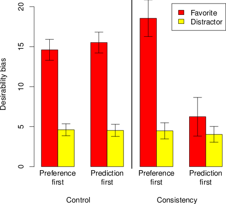
Figure 1: Mean desirability bias for both favorite and distractor
games, separately for priming condition (consistency primed versus
control) and for response order (Preference first versus
Prediction first). Error bars are SEs. Differences among
error bars reflect the different frequencies of observations:
three times as many observations for control as primed games and
seven times as many observations for distractor as favorite
games.
3 Results
3.1 Baseline desirability bias
The DB was calculated as the difference between a participant’s
Predicted Likelihood of the preferred team’s victory and the
corresponding likelihood estimated by TeamRankings.com. For games
involving participants’ favorite teams, the mean DB over control games
was 15.06 (SD = 20.72), a value well above zero
(t(542) = 16.94, p < .001, d = 1.46). This
value amounted to a preference-driven upward bias of .15 in
participants’ predicted probability that their favorite team would
win. Its magnitude might be judged relative to the .06 probability
increment over random performance achieved by TeamRanking.com’s
predictions across the entire 2014 baseball season (or the .08
increment for the games in this study).
Before proceeding to the main results of the effect of priming CC on
the DB, we tested for a difference in the DB between the two control
conditions that differed only by whether Preference or Prediction was
the first response. Recall that because there was no effect of serial
position, each control was comprised of the first 4 (unprimed) games
in the primed conditions (Columns 1–2 in Table 1) and all 8 games in
the controls that tested for an effect of serial position (Columns
3–4). For all control games involving a favorite team, the mean DB
when Preference was the first response was 14.61 (SD = 20.79)
and for Prediction-First was 15.52 (SD = 20.68). These two
means are shown as the two leftmost red (dark) bars in Figure 1. They
were not reliably different, t(541) = .51, p = .61,
d = .04. We note that this absence of a difference in
response order for unprimed participants is also a substantive result:
The order of Preference and Prediction did not matter in our sports
context when the consistency goal was not activated.
3.2 Priming cognitive consistency
The two principal research questions were (1) did priming CC increase
the DB when the Preference response preceded the Prediction response
and (2) how did reversing the order of these two responses affect this
bias? Because response order made no difference for control games, we
combined Preference-first (14.61) and Prediction-first (15.52)
controls, yielding a combined control mean of 15.06. Our two research
questions could then be answered by a one-way ANOVA predicting DB with
condition as a 3-level factor (Control, Primed Preference-first, and
Primed Prediction-first) and, more directly, the two planned
comparisons of the corresponding two primed groups against the unified
control.
Before proceeding with this computation, we needed to consider the
possible role of team success as a confounding factor. That is, might
team success have influenced the DB separately from either priming the
consistency goal or response order? On the one hand, if a favorite
team was relatively successful (unsuccessful), participants may have
felt more (less) confident in their team’s next victory and exhibited
a larger (smaller) DB. In either case, the DB might have been
positively correlated with team success. On the other hand, because
the baseline prediction of successful teams started relatively high,
there was less room both for the DB to elevate the Predicted
Likelihood and also for priming CC to increase it even further. In
such a case, the correlation between team success and the DB might
have been negative. Any systematic effect of team success, whether
positive or negative, should be removed from the statistical tests. To
assess team success, we used the 2014 full-season proportion of games
won, which ranged from a high of .605 for the Los Angeles Angels to a
low of .395 for the Arizona Diamondbacks. For favorite games, the
correlation between this measure of team success and the DB was r(708)
= .35, p < .001. Thus, in spite of a plausible concern about how much
higher the DB could rise when it was already likely to be higher for
more successful teams, the data showed that it still rose more for the
successful teams.
After including favorite-team success measured by win proportion as a
covariate, we computed the one-way ANCOVA described above. Results
yielded a significant effect of Condition F(2, 704) = 6.68,
p = .001, partial η2 = .019, as well as a significant
effect of team success F(1, 704) = 98.68, p < .001,
partial η2 = .123. However, the answers to our two research
questions lay in the two planned comparisons between the primed
conditions and the control. First, the mean DB when Preference was the
first required response was 18.55 (SD = 21.98), as shown in
Figure 1. A planned comparison confirmed that this value was
significantly higher than the control mean (15.06), t(704) =
2.00, one-sided p = .023, d = .16. Thus, as
expected, priming CC increased the DB when Preference was the initial
response.
The answer to the open question of the impact of CC on the DB when
Prediction was the first response was a reduction from the 15.06 of
the control to 6.24 (SD = 24.37). This decrease of 59% in
the magnitude of the DB was significant, t(704) = 2.77,
two-sided p < .01, d = .22. Despite the decrease,
the DB for this condition remained significantly above zero,
t(77) = 2.26, one-sided p = .018, d =
.23.4
Table 2: Condition and strength of preference predicting desirability bias in games involving favorite teams.
Predictor
B
[95% CI]
SE
Wald χ2
p
Intercept
15.03
[13.30, 16.77]
0.89
288.14
< .001
Pref-first
3.44
[–1.23, 8.11]
2.38
2.08
.150
Pred-first
-8.68
[–13.58, –3.78]
2.50
12.04
.001
Preference strength
.25
[.15, .34]
0.05
24.32
< .001
Pref-first X Preference strength
.27
[.01, .52]
0.13
4.28
.039
Pred-first X Preference strength
-.15
[–.39, .09]
0.12
1.45
.229
Note. Pref = Preference; Pred = Prediction. Both Preference and Prediction refer to primed games.
The Strength of Preference variable was mean-centered (M = 84.74) for this analysis.
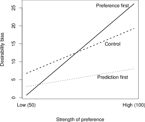
Figure 2: Regression lines for desirability bias on strength of preference by condition.
For completeness, we replicated the above analysis including the
distractor (i.e., non-favorite) games by adding Favorite (favorite
versus distractor) as a third factor. The means of the four main
conditions for the distractor games are also shown in Figure 1. The
analysis, available in the
Supplemental
Materials, revealed no effects either of priming or response order
on DB for the distractor games. There was a non-zero DB for these
games (4.41 over the two control conditions). However, the preferences
for winners that drove this mean DB might have been driven by negative
desires for a team to lose (e.g., a rival of the favorite team) as
much as by a second favorite. The mixed sources of preference combined
with the absence of reliable differences over conditions discouraged
further exploration of the distractor data.
3.3 DB and strength of preference
Because the DB is driven by the strength of the desire, which in our
experiment was the Strength of Preference for the favorite game, there
should have been a positive relation between the magnitudes of
Strength of Preference and the associated DB. A regression with
Strength of Preference (mean centered), Condition (dummy codes for
Preference-first primed and Prediction-first primed, with Control as
the excluded category), and their interactions predicting DB was
performed to determine whether the consistency and order manipulations
influenced the relationship between Strength of Preference and DB (see
Table 2). Figure 2 displays the mean DB for different levels of the
Strength of Preference and the resulting regression lines. As shown in
Figure 2, there was a positive relationship between Strength of
Preference and DB for control participants (r(543) = .21,
two-sided p < .001). The relationship was significantly
different from zero (r(87) = .44, two-sided p <
.001) and reliably stronger for those in the Preference-first primed
condition, z = 2.21, two-tailed p = .027. When the
response order was reversed, the relation between DB and Strength of
Preference (r(78) = .08, two-sided p = .46) is shown
by the lowest line in Figure 2. This relationship was not
significantly different from zero, but was also was not significantly
different from the control group, z =1.08, two-sided
p = .28.
We also replicated the above analysis for all games (favorites and
distractors). We did not include Favorite as a separate factor due the
problem of collinearity between favorites and Strength of
Preference. The analysis (see Table S6 in
Supplemental
Materials) revealed a marginal main effect of Prediction-First with
less DB in this condition. There was also a Preference-first primed X
Strength of Preference interaction, such that those in the
Preference-first primed condition with a stronger Strength of
Preference showed greater DB, and a marginal Prediction-first primed X
Strength of Preference interaction with a reduction of the
relationship between Strength of Preference and DB. Overall, these
results for all games were rather similar to those in Table 2 for
favorite games.
3.4 Uneven DB over teams
Because our method did not randomly assign participants to a favorite
team, differences in the magnitude of the DB across teams might have
created an uneven baseline DB across conditions if random assignment
failed to equate the distribution of favorite teams over
conditions. This would amount to starting points from which the
effects of priming were estimated that may have been different for
each condition. In fact, there were such differences across teams and
conditions. For instance, for the Yankees-Rangers game, in the control
condition the mean DB of the 33 Yankees fans was 23.76 while that of
the 7 Rangers fans was –7.54. In the Preference-First primed
condition, there were 8 Yankee fans (Mean DB = 35.83) and 1 Ranger fan
(DB = –15.83), while in the Prediction-First primed condition there
were 2 Yankee fans (mean DB = 25.83) and 5 Rangers fans (mean DB =
–24.83). In order to determine whether this uneven distribution of
baseline DB over the 30 teams accounted for our (between-condition)
effects, we constructed an alternative measure of DB (suggested by a
reviewer) that normalized the DB for the two teams in each game. To
get this adjusted DB, we regressed participants’ Predicted Likelihood
that the home team will win for each individual game (including both
favorites and distractors) on their Strength of Preference for a home
team win (transformed such that –100 was the maximum preference for
the visiting team and 100 was the maximum preference for the home
team). The intercept from each regression represented the likelihood
estimate of a participant who held a neutral preference for either
team. The difference between this intercept and each participant’s
actual Predicted Likelihood for that game estimated the (adjusted)
level of the DB. Next, this value was signed positively when
participants preferred the home team and negatively when they
preferred the visiting team. Finally, these scores were z-transformed
separately for each game so that all games could be compared on the
same basis. Because this adjusted DB was standardized within-game, an
unequal preference for one team within a condition should have been
removed. For instance, the standardized DB the for Yankee fans in the
control condition was 0.22 while that of Rangers fans was 0.23
(compared to the corresponding raw values of 23.76 and –7.54 reported
above).
An ANOVA was performed on this adjusted DB score with Condition as the
independent variable, again controlling for team win proportion. The
significant effect of Condition remained, F(2, 704) = 5.64,
p = .004, partial η2 = .016. More importantly, the mean
adjusted DB for the control games was 0.43 (SD = 1.10), a
value significantly lower than that for Preference-first primed games
M = 0.66 (SD = 1.10), t(704) = 1.81,
one-sided p = .035, d = .14. Also, the control value
was significantly higher than that for Prediction-first primed games
M = 0.04, (SD = 1.30), t(704) = 2.56,
two-sided p = .011, d = .21. Given the similarity
between results for both the raw and adjusted DB measures, an
unbalanced distribution of fans across conditions did not account for
the effects of priming and response order. Therefore, subsequent
analyses use the original, unadjusted DB measure.
3.5 What caused the reduction of the desirability bias when
prediction was first?
The results when Prediction was the first response enabled us to
distinguish among the three potential processes, viz., the continued
dominance of Preference, consistency with game-specific facts, and the
bandwagon effect. The observed 59% reduction of the DB when CC was
primed and Prediction was the first response (see Figure 1) supported
the consistency-with-fact process, which led to a more accurate
Prediction and, therefore, a lower DB. The observed reduction in DB
simultaneously disqualified the continued dominance of Preference,
which required an increase in the DB. The remaining possibility, the
bandwagon effect (under consistency priming) required a corresponding
decrease in the reported Strength of Preference (compared to the
control condition). Always restricting the analysis to when Prediction
came first, the mean Strength of Preference in the control and primed
conditions, respectively, was 84.88 (SD = 17.82) and 83.62
(SD = 20.98). Their difference, though directionally
compatible with some power of Prediction to lower the Strength of
Preference, was not statistically reliable (t(619) = 0.57,
p = .72, d = .05). The absence of reliable evidence
that estimating Prediction first caused a compatible change in the
Strength of Preference eliminated the bandwagon effect from
consideration. Thus, the pattern of results supported only the
consistency-with-facts process as the explanation for the observed
effect of priming on the DB when Prediction was the first response.
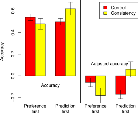
Figure 3: Accuracy is the proportion of (favorite) games correctly
predicted by participants. Adjusted accuracy is accuracy minus the
baserate of correct predictions from TeamRankings for the same
games.
3.6 Prediction accuracy
Finally, we examined whether the increase in DB in the
Preference-first primed condition led to a corresponding decrease in
accuracy in predicting game outcomes and whether a decrease in DB in
the Prediction-first primed condition actually led to increased
accuracy. The proportions of participants’ correct predictions, our
measure of accuracy (0 = incorrect, 1 = correct), are shown in the
left panel of Figure 3 for the four conditions formed by the 2x2
design of consistency priming and response order. However, because the
distribution of favorite teams differed across conditions, the
baserates of accuracy (from TeamRankings) were likely also to differ
across conditions. Thus, to evaluate the effect of priming and
response order on participants’ accuracy, we needed to subtract the
TeamRankings’ prediction (also 0 = incorrect, 1 = correct) from the
participants’ accuracy for each of the four conditions. These
differences in proportions correct created the four adjusted accuracy
scores in the right panel of Figure 3. Note that because the
participants’ accuracies were distorted by the DB, they were expected
to be lower than TeamRankings’ predictions. As a result, the adjusted
accuracy scores were expected to be negative.
A Prime X Order ANOVA over these adjusted accuracy scores yielded a
significant 2-way interaction, F(1, 704) = 10.82, p
= .001, partial η2 = .015. Adjusted accuracy was greater in the
Prediction-first primed condition (.06 above the proportion of correct
predictions made by TeamRankings) compared both to its corresponding
control condition (F(1, 704) = 8.54, p = .004,
partial η2 = .012) and also to the Preference-first primed
condition (F(1, 704) = 6.76, p = .010, partial
η2 = .010). Remarkably, this adjusted accuracy for
Prediction-first primed was positive. However, this result may well be
no more than a statistical anomaly (the .06 did not differ reliably
from zero, t(77) = 0.93, p = .356 d =
.21). The Preference-first primed prediction’s adjusted accuracy
(–.18) was the lowest of all, which is not surprising because this
condition exhibited the highest DB. Its value was marginally less
accurate than the corresponding Preference-first control
(F(1, 704) = 2.91, p = .089, partial η2 =
.004). Finally, we compared the two control conditions. Unlike prior
results, which indicated no difference between Orders in the control
condition, Preference-first control predictions were significantly
more accurate than Prediction-first controls, –.06 versus –.17,
F(1, 704) = 4.40, p = .036, partial η2=
.006). This finding represented a reversal of the effect in the primed
condition. Additional analyses that used either logistic regression or
Brier scores yielded similar results (see the
Supplemental
Materials).
Given the ability of priming in the Prediction-first condition to
lower the DB (relative to the control condition), it was not
surprising that priming when Prediction came first yielded the best
accuracy. That this accuracy was (nonsignificantly) superior to the
TeamRankings’ baserate should be conservatively interpreted as an
effect of variability in observed accuracy with small
samples. Nonetheless, these results provide additional evidence for
increased consistency with the facts as the process by which DB was
decreased in this condition.
4 Discussion
Our results enlarge the theoretical understanding of the DB in two
ways. First, they increase our knowledge of the possible causes of
this well-known bias, both by adding the goal of CC as a new cause and
by supporting previous claims of CC’s role in three other causal
mechanisms (Krizan & Windschitl, 2007). The nondirectionality of CC
might seem to preclude its driving a directional phenomenon like the
DB. However, our experimental paradigm illustrates how a direction can
be devised both by one belief’s being dominant (Preference in the case
of the DB) and also by inserting a direction-inducing stimulus
(game-specific facts in the baseball context). The nondirectionality
of the consistency goal stems, in part, from its nature as a process
goal in contrast to an outcome goal (van Osselaer et al., 2005). The
latter type of goal supports targeted outcomes, such as consuming
fewer calories, finding the cheapest airfare, or emphasizing an
automobile’s safety in bad weather. In contrast, process goals like
saving effort and enjoying the experience (of the process) do not
target any particular outcome. CC is a process goal and exhibits this
category’s typical property of nondirectionality.
The second contribution to understanding the DB is less theoretical
and more pragmatic. The combination of priming CC and asking the
prediction question first reduces this bias by more than half. This
tactic of prediction first might be contrasted with previous methods
that tap cognitive resources for reducing bias (Bélanger, Kruglanski,
Chen & Orehek, 2014; Lench & Bench, 2015). We also note that the
present data suggest that response order will not affect the DB unless
CC is activated above its chronic baseline. How often this occurs
under natural circumstances is an open question.
The observed role of CC may apply not only to judgmental biases but
also to any other psychological phenomenon that involves beliefs. For
instance, Chaxel et al. (2016) demonstrated that CC can reduce an
implicit attitude, the bias against overweight people. They did this
by requiring a statement of the explicit attitude (which is less
biased), then priming CC, and finally assessing the implicit attitude
(using the IAT). Priming CC moved the (more biased) nonconscious
implicit attitude to greater agreement with the previously activated
(less biased) explicit attitude. It must be repeated that the
demonstration of the impact of the CC goal both on the DB and in
Chaxel et al. relied on the experimental activation of this goal. Our
results showed that without this manipulated activation, there was no
difference caused by the order of the Preference and Prediction
responses. It seems that under chronic, background levels of
activation, the consistency goal may have little or no effect on the
DB or, possibly, other JDM phenomena.
The use of the conundrum-based method for priming CC is relatively
new. While this method manipulates the consistency goal, there is a
second and equally novel method for measuring the activation of this
goal during task performance. Carlson, Tanner, Meloy and Russo (2014)
interrupted a task and asked for a report of goal activation on a
continuum. They showed that a successful report of goal activation
requires both assessment during a task (as opposed to a post-task
report based on immediate memory) and a continuous response scale (as
opposed to a yes-no report of a goal as active or not active). The
combination of goal manipulation, as in the above study, and goal
measurement, using Carlson et al.’s method, promises testing of
goal-based theories of behavior that is more rigorous than heretofore.
References
Ashworth, J. Geys, B. & Heyndels, B. (2006). Everyone Likes a Winner: An Empirical Test of the Effect of Electoral Closeness on Turnout in a Context of Expressive Voting ,Public Choice, 128(3/4), 383–405.
Babad, E. (1987). Wishful thinking and objectivity among sports fans. Social Behaviour, 2, 231–240.
Bélanger, J. J., Kruglanski, A. W., Chen, X., & Orehek, E. (2014). Bending perception to desire: Effects of task demands, motivation, and cognitive resources. Motivation and Emotion, 38, 802–814.
Chaxel, A. S., & Russo, J. E. (2015). Cognitive consistency: Cognitive and motivational perspectives. In Evan A. Wilhelms and Valerie F. Reyna (eds.), Neuroeconomics, Judgment, and Decision Making (pp. 29–48). New York, NY: Psychology Press.
Chaxel, A. S., Russo, J. E., & Wiggins, C. E. (2016). “A Goal-priming Approach to Cognitive Consistency: Applications to Social Cognition,” Journal of Behavioral Decision Making, 29, 37–51.
Carlson, K. A., Tanner, R. J., Meloy, M. J., & Russo, J. E. (2014). Catching Goals in the Act of Decision Making,” Organizational Behavior and Human Decision Processes, 123, 65–76.
Cialdini, R. B., Borden, R. J., Thorne, A., Walker, M. R., Freeman, S., & Sloan, L. R. (1976). Basking in reflected glory: Three (football) field studies. Journal of Personality and Social Psychology, 34, 366–375.
Dolan, K. A., & Holbrook, T. M. (2001). Knowing versus caring: The role of affect and cognition in political perceptions. Political Psychology, 22, 27–44.
Elster, J. (1983). Sour grapes: Studies of the subversion of
rationality. New York: Cambridge University Press.
Fishbach, A., & Ferguson, M. F. (2007). The goal construct in social psychology. In A. W. Kruglanski and E. T. Higgins (Eds.), Social psychology: A Handbook of basic principles (pp. 490-515). New York, NY: Guilford Press.
Forster, J., Liberman, N., & Friedman, R. (2007). Seven principles of goal activation: A systematic approach to distinguishing goal priming from priming of non-goal constructs. Personality and Social Psychology Review, 11(3), 211–233.
Gawronski, B., & Strack, F. (2012). Cognitive Consistency: A Fundamental Principle in Social Cognition. New York, NY: The Guilford Press.
Hirt, E. R., Zillmann, D., Erickson, G. A., & Kennedy, C. (1992). Costs and benefits of allegiance: Changes in fans’ self-ascribed competencies after team victory versus defeat. Journal of Personality and Social Psychology, 63, 724–738.
Krizan, Z., & Windschitl, P. D. (2007). The influence of outcome desirability on optimism. Psychological Bulletin, 133, 95–121.
Lench, H. C., & Bench, S. W. (2015). Strength of affective reaction as a signal to think carefully. Cognition and Emotion, 29, 220–235.
Markman, K. D., & Hirt, E. R. (2002). Social prediction and the “allegiance bias”. Social Cognition, 20, 58–86.
Massey, C., Simmons, J. P., & Armor, D. P. (2011). Hope over experience: Desirability and the persistence of optimism. Psychological Science, 22, 274 – 281.
Mehrabian, A. (1998). Effects of poll reports on voter preferences, Journal of Applied Social Psychology, 28, 2119–2130.
Morwitz, V. G., & Pluzinski, C. (1996). Do polls reflect opinions or do opinions reflect polls? The impact of political polling on voters’ expectations, preferences, and behavior. Journal of Consumer Research, 23, 53–65.
Muren, A. (2012). Optimistic behavior when a decision bias is costly: An experimental test. Economic Inquiry, 50, 463–469.
Price, P. C. (2000). Wishful thinking in the prediction of competitive outcomes. Thinking and Reasoning, 6, 161–172.
Serra, M. J., & DeMarree, K. G. (2016). Unskilled and unaware in the
classroom: College students’ desired grades predict their biased grade
predictions. Memory and Cognition, 44, 1127–1137.
Shepperd, J. A., Waters, E. A., Weinstein, N. D., & Klein, W. M. P. (2015). A primer on unrealistic optimism. Current Directions in Psychological Science, 24, 232–237.
Simmons, J. P. & Massey, C. (2012). Is optimism real? Journal of Experimental Psychology: General, 141, 630–634.
Simmons, J. P., Nelson, L. D., Galak, J. & Frederick, S. (2011). Intuitive Biases in Choice versus Estimation: Implications for the Wisdom of Crowds. Journal of Consumer Research, 38, 1–15.
van Osselaer, S. M.J., Ramanathan, S., Campbell, M. C., Cohen, J. B.
Dale, J. K., Herr, P. J., Janiszewski, C., Kruglanski, A. W., Lee,
A. Y., Read, S. J., Russo, J. E., & Tavassoli, N. T. (2005), Choice
Based on goals. Marketing Letters, 16(3/4), 335–346.
Williams, S. (2009). Sticky expectations: Responses to persistent over-optimism in marriage, employment contracts, and credit card use, Notre Dame Law Review, 84, 733.
Windschitl, P. D., Scherer, A. M., Smith, A. R., & Rose, J. P. (2013). Why so confident? The influence of outcome desirability on selective exposure and likelihood judgment, Organizational Behavior and Human Decision Processes, 120, 73–86.
Cornell University,
443 Sage Hall, Samuel Curtis Johnson Graduate School of Management, Cornell University, Ithaca, NY 14853-6201. E-mail: jer9@cornell.edu.
Questions 1, 5, and
10, with the correct answer bolded, were: (1) This team has won 27
World Series Championships, the most in MLB history: Los Angeles
Dodgers, Atlanta Braves, New York Yankees, or Boston Red
Sox; (2) The last realignment of MLB divisions was before the 2013
season, seeing this team switch leagues: Houston Astros,
Seattle Mariners, Colorado Rockies, or Philadelphia Phillies; (3)
The metric ERA+ adjusts a pitcher’s ERA (earned run average)
according to the pitcher’s ballpark and the league’s run scoring
environment. ERA+ is normalized so that a score of
reflects the league average: 0, 4, 50, or
100. (See Supplemental Materials for the
full quiz).
The use of a conundrum to
activate the goal of CC is still new. Its rationale, validation, and
application are fully presented in Chaxel et al. (2016). Briefly,
the kind of conundrum used to prime consistency contains two facts
that cannot easily be reconciled. In the present study those facts
were “most people today strongly reject prejudiced social beliefs
from a hundred years ago on intrinsic grounds” and “there is
basically no intrinsic difference between people today and people
from the beginning of the last century.” Participants’ effort to
resolve the inconsistency between these two statements activates the
goal of CC. Because they cannot be (easily) reconciled, this goal
remains activated and influences the performance of the next
task. Further, the level of activation is increased by the insertion
of an intervening task that frustrates the achievement of the
consistency goal (Chaxel & Russo, 2015). Thus, the goal activation
method consisted of two tasks, resolving a conundrum and a
goal-frustrating filler task.
Note
that random assignment of participants to the four conditions
represented by the four columns in Table 1 was not equivalent to
the ideal test of the DB described by Krizan and Windschitl
(2007). In that test, participants are assigned randomly to
Preferences, not conditions. In our sports context, random
assignment of each participant to a favorite team would mean
something like instructing a participant that their favorite team
was to be, say, “the Boston Red Sox for the purposes of this study”.
Whether such instructed randomization would have succeeded is an
open question. However, it would have required not only the
pretended commitment to the (randomly) assigned team, but also
participants’ suspension of their allegiance to their true
favorite. We chose the natural association between participants and
their respective favorite teams. This made the experiment both more
realistic and more validly conclusive if null results were found
(instead of blaming a weak realization of the randomly assigned team
preference). However, one downside of the random assignment of
subjects to conditions rather than to teams is that the frequency
distribution of favorite teams over conditions could be uneven. The
possible effect of this imbalance on the results is addressed by an
alternate measure of the DB that adjusts for it, as described in the
presentation of the results.
For completeness, the one-way ANOVA used to answer the
two central research questions was partitioned into a 2x2 ANOVA by
keeping separate the two control conditions. This analysis (provided
in the Supplemental
Materials) yielded results similar to those reported
above. Specifically, both tests of differences between the two
primed conditions and their respective controls yielded
statistically significant effects.