| Figure 1: The appearance of one choice trial. |

Judgment and Decision Making, Vol. 11, No. 1, January 2016, pp. 75-91
Risky Decision Making: Testing for Violations of Transitivity Predicted by an Editing MechanismMichael H. Birnbaum* Daniel Navarro-Martinez# Christoph Ungemach$ Neil Stewart ** Edika G. Quispe-Torreblanca ** |
Transitivity is the assumption that if a person prefers A to B and B to C, then that person should prefer A to C. This article explores a paradigm in which Birnbaum, Patton and Lott (1999) thought people might be systematically intransitive. Many undergraduates choose C = ($96, .85; $90, .05; $12, .10) over A = ($96, .9; $14, .05; $12, .05), violating dominance. Perhaps people would detect dominance in simpler choices, such as A versus B = ($96, .9; $12, .10) and B versus C, and yet continue to violate it in the choice between A and C, which would violate transitivity. In this study we apply a true and error model to test intransitive preferences predicted by a partially effective editing mechanism. The results replicated previous findings quite well; however, the true and error model indicated that very few, if any, participants exhibited true intransitive preferences. In addition, violations of stochastic dominance showed a strong and systematic decrease in prevalence over time and violated response independence, thus violating key assumptions of standard random preference models for analysis of transitivity.
Keywords: transitivity, true and error models, dominance, stochastic
dominance, preference models
Transitivity of preference is a fundamental property that is regarded by many as a property of rational decision making. Transitivity is the premise that, if A is preferred to B and B is preferred to C, then A is preferred to C. Some descriptive models of risky decision-making satisfy transitivity and other models violate it systematically, so testing transitivity allows us to compare the descriptive adequacy of rival theories.
If each prospect creates an independent subjective value and if people make decisions by comparing these values — as in expected utility (EU) theory, cumulative prospect theory (CPT) or the transfer of attention exchange (TAX) models, among others (Birnbaum, 2008b; Tversky & Kahneman, 1992) — choices would satisfy transitivity of preferences, apart from error. However, if people compare prospects by comparing features of the prospects — as assumed by regret theory (Loomes & Sugden, 1982), similarity theory (Leland, 1998), or lexicographic semiorder models (Tversky, 1969), including the priority heuristic (Brandstätter, Gigerenzer & Hertwig, 2006) — they might violate transitivity.
Although some authors thought there was evidence of systematic intransitivity predicted by intransitive models (Tversky, 1969; Loomes, Starmer & Sugden, 1991; Loomes, 2010), the evidence presented was not decisive because the data could also be explained by transitive models. Disputes arose concerning Tversky’s (1969) data analysis (Iverson & Falmagne, 1985; Myung, Karabatsos & Iverson, 2005). In particular, the claimed cases for intransitive preferences did not properly account for the possibility of mixtures of true preferences (May, 1954) or of mixtures of true preferences perturbed by response errors (Birnbaum, 2011). For example, a mixture of transitive preference patterns could have produced data interpreted by Tversky (1969) as intransitive.
Recent studies attempted to replicate Tversky’s (1969) study, but the previously reported pattern of intransitive behavior was not replicated (Birnbaum & Gutierrez, 2007; Birnbaum & Bahra, 2012b; Regenwetter, Dana & Davis-Stober, 2011); few individuals tested in these new studies showed data matching predictions of lexicographic semiorders or the priority heuristic (Brandstätter et al., 2006).
In fact, other experiments showed substantial, systematic violations of critical properties implied by a general family of lexicographic semiorders (Birnbaum, 2010), including the priority heuristic (Brandstätter et al., 2006), so this family of models could be rejected as an accurate descriptive model.
When regret theory has been put to the test, violations predicted by regret theory do not appear (Birnbaum & Schmidt, 2008), even in experiments where a general model that includes regret theory, majority rule, and the model of Loomes (2010) as special cases implies that intransitivity must occur (Birnbaum & Diecidue, 2015, Experiment 6).
However, failures to find evidence of intransitivity predicted by lexicographic semiorders, by the priority heuristic, regret theory, majority rule, or by similarity theory, and findings that violate those intransitive models, do not guarantee that transitivity is always satisfied.
People might also violate transitivity by another mechanism: people might use different decision rules for different choice problems. For example, if people use an editing rule for some choice problems and not for others, they could easily violate transitivity. Because prospect theory in its simplest form implied that people would violate transparent dominance, Kahneman and Tversky (1979) theorized that people look for dominance and satisfy it whenever the relation is apparent. But they did not state a theory or even a list of conditions stating when dominance would or would not be apparent.
Birnbaum, Patton and Lott (1999) proposed a paradigm where violations of transitivity would occur if people systematically violated dominance in complex choice problems and satisfied it in simpler choices. This paradigm was in turn based on Birnbaum’s (1997, 1999a) recipe for creating violations of stochastic dominance. This recipe was devised to test between CPT, which must satisfy stochastic dominance, and TAX, which violates it in specially constructed choice problems.
Like transitivity, stochastic dominance is widely regarded as a normative principle of decision making, but some descriptive models violate this property and others satisfy it. With the recipe, a majority of undergraduates violated first order stochastic dominance (Birnbaum, 1999b, 2004, 2005, 2008b; Birnbaum & Navarrete, 1998), confirming the predictions of the TAX model and refuting CPT. Understanding the recipe is important for understanding how it might be used to create violations of transitivity.
Birnbaum’s (1997) recipe was designed on the basis of configural weight models, including the RAM and TAX models, which can violate stochastic dominance in specially constructed choices between three-branch gambles. A branch of a gamble is a probability-consequence pair that is distinct in the presentation to the decision maker.
Consider the following example: Start with G0 = ($96, .90; $12, .10), which is a two-branch gamble with a .90 probability to win $96 and otherwise win $12. Construct a better, three-branch gamble, G+ = ($96, .90; $14, .05; $12, .05), by splitting the lower branch of G0 (.10 probability to win $12) into two splinters of 0.05 to win $12 and then increase the value of one of the splinters to 0.05 to win $14. Next, construct a gamble worse than G0 by splitting the upper branch of G0 (and diminishing a splinter) as follows: let G– = ($96, .85; $90, .05; $12, .1); note that G+ dominates G0 which dominates G–.
In Birnbaum’s configural weight models (RAM and TAX), splitting the upper branch gives more weight to the upper branches making a gamble better (despite the small decrease in value of the higher consequence from $96 to $90) and splitting the lower branch of a gamble gives greater weight to lower values, making it worse (despite the small increase from $12 to $14). Thus, these models allow violations of stochastic dominance in choices constructed from this recipe.1
Birnbaum and Navarrete (1998) included four variations of G– versus G+, constructed from the same recipe and embedded among a large number of other choice problems, and found that about 70% of the undergraduates tested violated dominance by choosing G– over G+. Such violations of first order stochastic dominance contradict cumulative prospect theory (CPT), even with any monotonic value function of money and any decumulative weighting function of probability. The configural weight models used to design the tests correctly predicted the majority violations.
Birnbaum (1999b) replicated this effect with more highly educated participants and found lower rates of violation, but rates still quite large for persons with college degrees (about 60%) and among those with doctorates (about 50%). Violation rates were higher among females than males for both lab and Internet samples.2
However, when the gambles, G– and G+ are split again so that the choice is presented in canonical split form (in which the number of branches in the two gambles are equal and minimal and probabilities on corresponding ranked branches are equal), the violations nearly vanish. For example, GS– = ($96, .85; $90, .05; $12, .05; $12, .05) was chosen only about 10% of the time over GS+ = ($96, .85; $96, .05; $14, .05; $12, .05), even though this choice is objectively the same as that between G– and G+ (Birnbaum, 1999b, p. 400).
Although this reversal of preference due to splitting refutes the most general form of CPT, it is consistent with RAM and TAX models. These two phenomena (violations of dominance and violations of coalescing3) have now been replicated in more than 40 experiments, using more than a dozen different formats for representing probabilities and displaying choice problems (Birnbaum, 2004b; 2006; 2008b; Birnbaum & Bahra, 2012a; Birnbaum, Johnson & Longbottom, 2008; Birnbaum & Martin, 2003).
Birnbaum et al. (1999) theorized that, if people can detect dominance between G+ and G0 and between G0 and G–, and if they continued to violate it in the choice between G+ and G–, there would be a predictable violation of transitivity. Starmer (1999) independently investigated a similar prediction of intransitivity. Although both articles concluded there might be evidence of intransitivity, the experimental results of these two studies must be considered as ambiguous for two reasons: first, enough people violated dominance on one or the other of the simpler choices that a majority of participants did not violate transitivity as anticipated. Second, at the time of these earlier studies, the modern true and error (TE) model of choice responses had not yet been developed. That model provides a better method for analysis of the question of transitivity (Birnbaum, 2013).
There has been considerable discussion and debate concerning theoretical representation of variability of response in studies of choice, including how to test transitivity (Birnbaum, 2004, 2011; Birnbaum & Gutierrez, 2007; Birnbaum & Schmidt, 2008; Carbone & Hey, 2000; Hilbig & Moshagen, 2014; Loomes & Sugden, 1998; Regenwetter, Dana & Davis-Stober, 2011; Sopher & Gigliotti, 1993; Tversky, 1969; Wilcox, 2008).
Birnbaum (2004b) proposed that, if the each choice problem is presented at least twice to the same person in the same session, separated by suitable intervening trials, reversals of preference by the same person to the same choice problem can be used to estimate random error. This approach can be applied in two cases: (1) when variability in choice responses to the same choice problem might be due to true individual differences between people; this case is termed group True and Error Theory (gTET), and (2) when the model is applied to variability of responses within a single individual in a long study, called individual True and Error Theory (iTET). Birnbaum and Bahra (2012a, 2012b) applied these models to test transitivity, stochastic dominance, and restricted branch independence.
Response independence is typically violated by the TE models but must be satisfied by methods that were once used to test transitivity via properties defined on binary choice proportions, such as weak stochastic transitivity and the triangle inequality (e.g., Regenwetter et al., 2011). Response independence is the assumption that a response pattern, or combination of responses, has probability equal to the product of the probabilities of the component responses. Birnbaum (2011) criticized this approach because it assumed response independence but did not test that crucial assumption. Regenwetter, Dana, Davis-Stober and Guo (2011) and Cha, Choi, Guo, Regenwetter & Zwilling (2013) defended the approach of assuming iid (independent and identical distributions) in order to test binary choice proportions, but evidence is accumulating that iid is not empirically descriptive (Birnbaum, 2012, 2013; Birnbaum & Bahra, 2012a, 2012b).
Birnbaum (2013) presented numerical examples to illustrate how analyses based on binary response proportions (e.g., the triangle inequality) would lead to wrong conclusions regarding transitivity, in cases where TE models can make the correct diagnosis.
Therefore there are two important reasons to find out whether or not the assumption of response independence is empirically satisfied or violated: first, it must be satisfied if we plan to analyze binary response proportions to study formal properties of choice data; second, the empirical property is predicted to be satisfied by the random preference models and can be violated by TE models if people have a mixture of true response patterns. A third reason to test iid is that the statistical tests that have been proposed to analyze binary response proportions depend upon this assumption.
Birnbaum (2013) also showed how TE models can be used to do something not possible in other approaches based on binary response proportions; namely, it is possible to estimate the proportions of different response patterns in a mixture. This study will apply TE models to the analysis of transitivity in the situation studied by Birnbaum et al. (1999), where it had been theorized that a partially effective editor was used to detect dominance and may have created violations of transitivity.
There are three choice problems testing transitivity: G+ versus G0, G0 versus G–, and G+ and G–. Let 1 = satisfaction of stochastic dominance and 2 = violation of stochastic dominance in these choices. If people satisfy dominance in the first two choices and violate it in the third, the predicted intransitive response pattern is denoted 112. There are 8 possible response patterns: 111, 112, 121, 122, 211, 212, 221, and 222. In the TE model, the predicted probability of showing the intransitive pattern, 112, is given as follows:
| (1) |
P(112) is the theoretical probability of observing the intransitive response cycle of 112; p111, p112, p121, p122, p211, p212, p221, and p222 are the probabilities of these “true” preference patterns, respectively (these 8 terms sum to 1); e1, e2, and e3 are the probabilities of error on the G+G0, G0 G–, and G+G– choices, respectively. These error rates are assumed to be mutually independent, and each is less than ½.
There are seven other equations like Equation ?? for the probabilities of the other seven possible response patterns. Note that, if the only information available were the frequencies of these 8 response patterns, there would be 7 degrees of freedom in the data. However, we use 10 degrees of freedom for the parameters, so that, when this model fits, there would be many solutions. In order to provide constraint to identify the parameters and test the model, additional structure is needed. This can be accomplished by presenting each choice problem at least twice to the each participant in the same session (block of trials). Here, we present two versions of the same choice problems, which can be considered replications.
Therefore, in addition to the choice problems, G+G0, G0 G–, and G+G–, we present slight variations: F+ versus F0, F0 versus F–, and F+ versus F–, where F+, F0, and F– are gambles and choice problems constructed from the same recipe as G+, G0, and G–, respectively. Because each type of choice problem is presented twice in each block (counterbalanced for position, so a person has to switch response buttons to stay consistent), there are now 64 possible response patterns for all six responses within each block.
If error rates are assumed to be the same for choice problems G+G0, G0 G–, and G+G– as for choice problems F+F0, F0 F–, and F+F–, respectively, the probability of showing the same pattern, 112, on both versions in a block is the same as in Equation ??, except that each of the error terms, e or (1−e), are squared. In this way, one can write out 64 expressions for all 64 possible response patterns that can occur for six choice problems in one block.
When cell frequencies are small, one can partition these 64 frequencies by counting the frequency of each response pattern on both versions of the same choice problems (G and F) and the frequency of showing each of 8 response patterns in the G choices and not in both variations (denoted G only). This partition reduces 64 cells to 16 cells. The purpose of this partition is to increase the frequencies within each cell, in order to meet the assumptions of statistical tests, while still allowing tests of independence, TE model, and transitivity (Birnbaum, 2013).
The general TE model for this case has 11 parameters: 3 error rates (one for each choice problem) and 8 “true” probabilities. Because the 8 “true” probabilities sum to 1, they use 7 df, so the model uses 10 df to account for 16 frequencies of response patterns. The data have 15 df because they sum to the total number of participants. That leaves 5 df to test the general TE model. A computer program that performs the calculations for either iTET or gTET is included in Appendix B; it finds best-fit solutions to the parameters, performs conventional statistical tests as well as Monte Carlo simulations and uses bootstrapping to estimate confidence intervals for the parameters.
The transitive TE model is a special case of the general TE model in which the two probabilities of intransitive patterns are set to zero, p112 = p221 = 0. A set of data can (and typically would) still show some incidence of intransitive response patterns even when the “true” probabilities of intransitivity are zero, due to error. The gTET model allows us to estimate the percentage of people who used each preference pattern, including the pattern 112 predicted by the theory of a partially effective dominance detecting editor.
In each of three studies, participants viewed choices between gambles on computers in the lab and made responses (choices) by clicking one of two buttons to indicate which gamble in each pair they would prefer to play. All three samples used the same 40 choice problems and the same instructions, but slightly different procedures and different participants.
Each choice problem (each trial) was displayed as in Figure 1. A choice problem was described with respect to two urns, each of which contained exactly 100 otherwise identical tickets, with different prize values printed on them. A ticket would be drawn randomly from the chosen urn and the prize would equal the cash value printed on the ticket.
Figure 1: The appearance of one choice trial.
Instructions read (in part) as follows: “…after people have finished their choices, three people will be selected randomly to play one gamble for real money. One trial will be selected randomly from all of the trials, and if you were one of these lucky people, you will get to play the gamble you chose on the trial selected. You might win as much as $100. Any one of the choices might be the one you get to play, so choose carefully.” After each study, prizes were awarded as promised.
Participants were also instructed to work at a steady pace, as their times to make decisions would be recorded, but each person was free to work at his or her own pace for the time allotted. Therefore, different participants completed different numbers of trials.
Clicking the “next trial” link displayed the next choice problem on the computer and also started the clock, which was stopped when the participant clicked to choose one of the gambles. The timing was programmed via JavaScript (Birnbaum, 2001; Reimers & Stewart, in press). Instructions, stimuli, and HTML code (for one trial block) can be found at the following URL: http://ati-birnbaum.netfirms.com/Fall_13/rev_trans_ti_01.htm.
There were 40 choice problems in each block of trials.
The main design testing transitivity and stochastic dominance consisted of 8 choice problems with two variants each of the following 4 choices: G+ versus G–, G+ versus G0, G0 versus G–, and GS+ versus GS–. Positions of the dominant and dominated gambles were counterbalanced across the two versions of the problems (Participants had to press opposite response buttons to make the same choice response when dominant gamble was presented in the first or second position). In the first set, G0 = ($96, .90; $12, .10), G+ = ($96, .90, $14, .05; $12, .05), G– = ($96, .85, $90, .05; $12, .10), GS+ = ($96, .85; $96, .05; $14, .05; $12, .05), and GS– = ($96, .85; $90, .05; $12, .05; $12, .05); in the second set, F0 = ($98, .92; $4, .08), F+ = ($98, .92; $8, .04; $4, .04), F– = ($98, .88; $92, .04; $4, .08), FS+ = ($98, .88, $98, .04; $8, .04; $4, .04), and FS– = ($98, .88; $92, .04; $4, .04; $4, .04).
In addition, an “extreme” choice, H++ = ($97, .91; $16, .05; $15, .04) versus H-- = ($86, .80; $85, .05; $4, .15), was presented. This extreme choice was devised from the same recipe that generates violations of dominance, but values were so extreme that a person would likely satisfy dominance given certain parameters of the TAX model; however, if the participant ignored probability (or had extreme parameter values), she might still violate stochastic dominance in this choice; but if she attended to magnitudes of consequences and probabilities she would likely satisfy dominance. Note that all nine of these trials involve tests of first order stochastic dominance.
There were also 31 other choice problems that are treated as “warmups” and “fillers” with respect to the main purpose of this study. These trials were replications or variations of choice problems reviewed in Birnbaum (2004, 2008b, 2008c). These included two additional tests of “transparent” dominance (in which the probabilities were identical but the consequences differed or in which the consequences were identical but probabilities differed). We do not discuss the results of these problems here.
The 40 trials in each block were presented in restricted random orders, such that each pair of trials from the main design testing transitivity would be separated by at least three intervening “filler” problems. Note that 11 of the 40 choice problems in each block involved first order stochastic dominance; further, four of these problems were considered “transparent.”
The first study had 28 participants who served in a single session of 1 to 1.5 hours. Results indicated that the incidence of violation of stochastic dominance decreased over the course of the study. Study 2 was conducted with 54 new participants who served in a longer study with two, 1.5 hour sessions (one week apart), to see if this new finding would be replicated and perhaps extended. This group indeed showed a strong decline in the rate of violation over trials, but the sample was unusual, since it contained a majority of male participants, whereas the participant pool contained a majority of females. Therefore, a third sample was collected in the following semester with 18 additional participants to balance out the sample at 100 participants with 50 males and 50 females. All three studies yielded consistent descriptive conclusions and are combined in analyses that follow.
Table 1 shows the rates of violation of first order stochastic dominance in the four types of choice problem in the main design. Each percentage is based on 200 responses in the first block and 200 in the last block of each person’s data (100 participants and two versions of each choice problem).
Table 1: Percentage of violations of first order stochastic dominance in different choice problems. Each percentage is based on 100 choice responses by 50 participants, averaged over two variations within each block (G and F). First and last refer to each participant’s first and last blocks of data.
Choice Type Females First Last Males First Last
Table 1 shows that the new data replicate six previous findings (Birnbaum, 1999b; 2005; Birnbaum et al., 1999). First, the rate of violation of stochastic dominance in the choice between G+ and G– (and F+ versus F–) exceeds 0.5 in the first block of trials for both males and females. The overall rate, 64%, is significantly greater than 50% and not significantly lower than the previously reported rate of 70% for similar choice problems, participants, and procedures (Birnbaum, 2005). Stochastic dominance must be satisfied for any CPT, RDU or RSDU model with any utility function and any weighting function (Birnbaum & Navarrete, 1998). Therefore, these new results replicate previous findings that contradict these models.
Second, the rate of violation in the choice between GS+ and GS– is much smaller than that in the choice between G+ and G– even though these are objectively the same choice problem. This huge effect (64% violations versus 8%) of the form of a choice problem (coalesced or canonical split) contradicts both versions of prospect theory. Original prospect theory assumed that people use the editing operation of combination (Kahneman & Tversky, 1979; Kahneman, 2003), which converts GS+ to G+ and converts GS– to G–, so these choices should be equivalent. CPT (with any strictly monotonic value and probability weighting functions) implies that there can be no difference between these two forms of the same choice problems. Coalescing holds for any CPT, RDU or RSDU model with any utility function and any weighting function (Birnbaum & Navarrete, 1998). Therefore, these new results replicate previous findings that refute both versions of prospect theory.
Third, the rate of violation of stochastic dominance is higher for females than for males, as reported previously by Birnbaum (1999b).
Fourth, as reported in Birnbaum et al. (1999), rates of violation of stochastic dominance in the simpler choices against G0 are higher than one might anticipate from the notion that these choice problems would be “transparent,” and detected by a dominance detecting editor such as postulated by Kahneman and Tversky (1979).
Fifth, the rate of violation of stochastic dominance in the choice between G0 and G– is greater than that in the choice between G0 and G+, as found by Birnbaum, et al. (1999).
Sixth, the extreme choice problem between H++ and H-- showed 39% violations in the first block and 36% violations in the last block; these rates are significantly below 50% and significantly lower than rates of violation for G+ versus G– (65%) and F+ versus F– (62%) in the first block (z = 3.23 and z = 3.35, respectively), which are both significantly greater than 50%. These results agree with previous reports that rates of violation in such extreme variations of the recipe can be significantly lower and yet still substantial (Birnbaum, 2005, 2008b, p. 478). These results for the extreme choice (H++ versus H--) show that the theory that people simply ignore probability is not sufficient to account for the violations of stochastic dominance; if people ignored probability, the majority should continue to violate stochastic dominance in this choice, but the majority satisfies dominance in this case.
The fact that these six effects were replicated using new participants and a different format for displaying the choice problems is important for two reasons: first, it shows that previous findings did not depend on particular features of that study; second, it gives us confidence that our new findings, presented in the next sections, address the issues raised in the previous research.
Table 1 shows an important new finding: The average rates of violation in the choices between G+ versus G– and in G0 versus G– are substantially lower in the last block of trials than in the first. Figure 2 shows the proportion of violations in the choices between G+ and G– and between F+ and F– plotted against trial blocks for the first ten blocks. The decrease was observed in both males and females, as shown by the separate curves. Of 100 participants, 44 had fewer violations of stochastic dominance in these two choice problems on their last block than their first, and only 18 had more (z = 3.30). Summed over all six choice problems testing dominance and transitivity in the main design, there were 62 people who had fewer violations of dominance in the last block than in the first, compared to only 17 who had more violations in the last block than in the first (z = 5.06).
Figure 2: Violations of first order stochastic dominance (G+ vs. G– and F+ vs. F–) as a function of trial blocks, with separate curves for female and male participants. 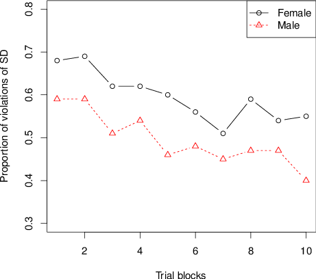
Such trends with increasing experience violate assumptions of independence and identical distribution (iid) that had been used in previous research to justify analysis of binary choice proportions when testing transitivity.
Appendix A applies Birnbaum’s (2012) statistical tests of iid to these data, which show significant violations of iid in individual subject data. These results (Figure 2 and Appendix A) add to the growing body of evidence against iid as descriptive of choice behavior (Birnbaum, 2013). Keep in mind that violations of iid raise the specter that conclusions from studies that are based strictly on binary response proportions are not definitive. Appendices B and C present further evidence, based on other implications of independence, against that model.
The decrease in choice proportion in Figure 2 might occur in this case because people are learning to conform to stochastic dominance during the study. It is possible that parameters representing probability weighting are changing, that people are learning to use an editor to detect stochastic dominance, which might create intransitivity, or that error rates for these choices are changing during the study. These interpretations of true intransitivity versus error are explored in the next sections via the TE models.
Table 2 shows the number of participants who showed each response pattern in the G choice problems, the F choices, and in both G and F in the first block of trials and in the last block. Responses are coded such that 1 = satisfaction of stochastic dominance and 2 = violation.
Table 2: Number of participants showing each response pattern in G+ versus G0, G0 versus G– and G+ versus G– choices, in the same tests based on F+, F0, and F–; and in both of the corresponding choices in the first and last blocks of trials. Responses are coded such that 2 = violation of stochastic dominance and 1 = satisfaction. The predicted intransitive pattern in which stochastic dominance is violated only in the choice between three-branch gambles is 112.
First Last Pattern 111 112 121 122 211 212 221 222 Total
The response pattern 111 satisfies both stochastic dominance and transitivity perfectly. This response pattern is predicted by CPT model with any monotonic value and probability weighting functions. The EU model is a special case of CPT and the TAX model, and EU also implies 111 with any utility function. In Table 2, the 13 under G in the first block shows that of the 100 participants, 13 of them satisfied stochastic dominance in all three choices, G0 versus G+, G0 versus G–, and G+ versus G–, respectively. Table 2 shows that 14 showed the same response pattern with F0 versus F+, F0 versus F–, and F+ versus F–. Only 4 participants showed response pattern 111 in both the G and F versions of the test of transitivity.
The TAX model with its prior specifications and parameters implies the response pattern 222, indicating violation of stochastic dominance in all three choice problems and satisfaction of transitivity. TAX with other parameters could also account for other transitive patterns; EU, for example, is a special case of TAX that implies the pattern 111. However, neither TAX nor CPT nor EU could account for violations of transitivity: patterns 112 or 221, because these models allow only transitive patterns.
The predicted pattern of intransitivity for the theorized dominance detector is 112 (satisfying stochastic dominance in the simpler choices of G+ versus G0 and G0 versus G– but violating stochastic dominance in the comparison of G+ and G–). Only 3 people showed this pattern in both the G and F tests in the first block and only 1 person in the last block of trials.
Table 2 indicates that 30 out of 100 participants showed the transitive response pattern 122, satisfying stochastic dominance in the choice between G+ and G0, and violating it in choice problems G0 versus G– and G+ versus G–. In the same row of Table 2, 29 people showed this response pattern when comparing F+, F–, and F0. The 15 under “G and F” in the fourth column indicates 15 repeated this same 112 pattern of responses in both G and F variants in the first block of trials.
The term “repeated” is used to indicate cases where a person showed the same response pattern in both F and G variants within a block. In the first block of data, the same response patterns were repeated in both the G and F tests in 30 of 100 cases and in the last block, response patterns were repeated (agreed) in 50 of 100 cases; this result shows that consistency within blocks increased over the course of the study.
The most frequent response pattern in the first block (and most frequently repeated pattern) was 122. These people violated stochastic dominance on the G+ versus G– choice (and F+ versus F–), violated it on G0 versus G– (and F0 versus F–); but they satisfied it on G0 versus G+ (and F0 versus F+). This 122 pattern was still prominent in the last block, but the most frequently repeated pattern in the last block was 111, which satisfies both transitivity and stochastic dominance in all three choice problems.
Table 3: Total number of blocks showing each response pattern in three choices: G+ versus G0, G0 versus G– and G+ versus G– choice problems and in the corresponding choices among F+, F0, and F–, and in both. Responses are coded such that 1 = satisfaction of stochastic dominance and 2 = violation. Pattern 112 is the predicted intransitive pattern.
Pattern G and F 111 112 121 122 211 212 221 222 Total
Table 3 shows the total frequencies of each response pattern, aggregated over all participants and all trial blocks. The most frequently repeated response patterns are 111 and 122, followed by 211 and 222. Of the 1037 blocks in which 111 occurred, 74% of the time (765) the same pattern was observed in both tests. Of the 902 blocks in which the response pattern was 122 in the G tests, 75% of the time it was repeated in both F and G. However, of the 242 blocks in which 112 was observed in the G test, it was observed in both variants only 18% of the time. The predicted intransitive pattern, 112, thus accounts for 7.6% of all response patterns, but only 2.5% of all cases where a person showed the same pattern in both tests within a block.
Table 4 shows the number of individuals who showed each response pattern as their most frequently repeated pattern. The sum across participants adds to 98 because two participants failed to repeat any pattern within a block. The three most commonly repeated patterns are the transitive patterns, 111, 122, and 222, accounting for 86% of all participants.
Table 4: Number of participants showing each modal repeated response pattern, tallied over blocks within each participant. The sum totals 98 because two participants did not show the same response pattern within any block in both G and F tests.
Pattern Number 111 48 112 2 121 1 122 35 211 6 212 2 221 1 222 3
Only one participant (Case #308) had the intransitive pattern 112 as the modal repeated pattern (across blocks). Case #308 repeated the 112 pattern 8 times and showed this pattern in one test or the other but not both on 13 other blocks (out of 27 blocks). Case #308 was therefore the best candidate for someone showing truly intransitive behavior. In addition, Case #218 repeated 112 and 111 equally often (5 times each, out of 19 blocks). But even if both of these two cases represented true, intransitive behavior, the prevalence appears to be small.
A search was made for transitory intransitive behavior, by counting participants who had the response pattern 112 as their second most frequently repeated pattern and who repeated it at least twice. There were only 6 cases of this type: one had 4 blocks out of 26 in which the 112 pattern was repeated in both tests. Five others had only 2 blocks with repeated 112 pattern. Of these 6 cases, 5 had 111 as the most frequently repeated pattern and one had 122 as the modal pattern. Certainly, some of this behavior could be due to chance, but even if we count all of these transitory cases as “real” and include the two cases above, it still means that only 8% of the sample showed evidence of even transitory intransitive behavior of the type predicted. The next sections apply TE models to estimate this incidence.
Table 5: Frequencies of response patterns for replicated choice problems in the first and last blocks of trials. Chi-Squares show the fit of independence and of the gTET model to the same frequencies. The TE model always fits at least as well as the independence model and markedly better in some cases, even though both models use the same number of degrees of freedom to fit the same four frequencies. (X = G or F).
Response pattern Parameters Type 11 12 21 22 p e XS+XS– first 92 1 6 1 5.80 0.00 0.06 5.12 XS+XS– last 82 7 8 3 4.10 0.00 0.12 3.75 X+X0 first 52 13 19 16 7.31 0.20 0.20 1.12 X+X0 last 70 14 4 12 23.77 0.13 0.11 5.25 X0 X– first 26 12 15 47 19.05 0.65 0.16 0.33 X0 X– last 50 13 4 33 44.10 0.39 0.11 4.52 X+X– first 19 16 19 46 6.06 0.75 0.23 0.26 X+X– last 38 18 13 31 14.47 0.44 0.19 0.80
Table 5 shows a breakdown of the frequency of each response pattern in the two tests of stochastic dominance for each of the replicated choice problems. Results are shown for the first and last blocks. Responses are coded so that 1 = satisfaction of dominance and 2 = violation of dominance. In Table 5, the response pattern 22 indicates that dominance was violated in both the G and F versions of the choice problem; the pattern 21 indicates a violation in the G variant but not the F version, respectively.
These frequencies can be fit to a simple gTET model. There are two parameters to estimate for each choice problem in each block, pi = the estimated true probability of violating stochastic dominance in problem i, and ei = the estimated error rate for that problem. Each choice problem is permitted a different true probability and a different error rate, so this model is not the so-called “tremble” model, which is a special case of the true and error model in which error rates for different choice problems are all equal, e1 = e2 = e3.
A rival theory to TE model assumes that responses (rather than errors) are independent. Both theories can be evaluated on the same data with Chi-Squares, and both are based on the same number of parameters and same degrees of freedom (Birnbaum, 2011, 2013). As shown in Table 5, gTET fits better than any model that assumes response independence, because all of the statistical tests of independence are large and significant.
As shown in Table 5, one can approximate the data for the GS+ versus GS– and FS+ versus FS– choices well using the assumption that no one truly violated stochastic dominance in these choices in both the first block and the last block. The results are consistent with the idea that all of the violations can be attributed to random error, with error rates of e = 0.06 and 0.12 in the first and last blocks, respectively. TAX, CPT, and EU all imply satisfaction of stochastic dominance in this choice problem, apart from error. In this choice problem response independence fits about as well as the TE model because the TE model satisfies independence when the true choice probability is either zero or one.
In contrast, Table 5 shows that in the choice problem between G+ and G–, the estimated rates of true violation of stochastic dominance in the first and last blocks are p = .75 and .44, respectively, with error rates of e = .23 and .19, respectively. The choice problems between G0 and G– show rates nearly as high, with p = .65 and .39 in the first and last blocks, respectively. These results violate CPT and EU (both of which must satisfy stochastic dominance and thus require p = 0), but remain compatible with the TAX model.
In the choice problem comparing G+ versus G0, the estimated rate of true violation in the first and last blocks are p = 0.20 and 0.13, respectively, with error rates of e = .20 and .11, respectively. This rate of violation is much smaller than that in the choice problem between G+ and G–, but not small enough to dismiss as zero. This is the only choice problem in Table 5 in which the majority preference in the first block does not match the prediction of the prior TAX model, which predicts violations of stochastic dominance in this problem.
Table 6: Fit of true and error model to frequencies of response patterns (data from Table 2). In the General TE models, all parameters are free; in the Transitive TE model, probabilities of intransitive patterns are fixed to zero (shown in parentheses). Confidence intervals (95% CI) are estimated from 10,000 Bootstrap samples drawn from the empirical data (2.5% of parameter estimates fell below the lower limit and 97.5% below the upper limit). The error rates, e1, e2, and e3 are for choices X0 versus X–, X+ versus X0, and X+ versus X–, respectively. The predicted intransitive response pattern was 112.
First block Last block Parameter p111 p112 p121 p122 p211 p212 p221 p222 e1 e2 e3 χ2
Response patterns for three choices testing transitivity were fit to the TE model, using methods described in the Introduction and Appendix B. An R-program that implements the calculations is included in the website with this article. (See also Birnbaum, 2013).
Estimated parameters for this gTET model and indices of fit are shown in Table 6 for the first and last blocks of data. There are 11 parameters to estimate (using 10 df), and there are 15 df in the data, leaving 5 df to test the model. In the transitive special case, p112 and p221 are fixed to 0 (shown in parentheses in Table 6).
The fit of the general TE model yielded χ2(5) = 1.44, which is not significant; for comparison, the fit of response independence to the same data yields, χ2(12) = 44.15, which is significant, p < .01. Thus, we can retain the TE model but we must reject models that imply response independence. These statistical conclusions were confirmed by Monte Carlo simulation under the TE model (Appendix B).
The estimated parameters show that the estimated incidence of the (predicted) intransitive pattern (p112) is only 0.08 in the first block of trials and 0.0 in the last block of trials.
Are the violations of transitivity in the first block (estimated p112 = 0.08) significantly greater than zero? When we fix p112 = p221 = 0, the model yields χ2(7) = 2.94. The difference in χ2 (between the indices of fit of general TE model and special case of transitivity) is χ2(2) = 2.94−1.44 = 1.50, which is not significant. Therefore, we can retain transitivity for both first and last blocks.
What percentage of people might have been intransitive, given these data? The 95% confidence intervals on the parameter estimates (Table 6) were generated via bootstrapping (Appendix B). The 95% confidence interval on p112 in the first block of trials ranges from 0 to 0.21. In the last block of trials, estimated p112 = 0 and falls between 0 and 0.05 with 95% confidence. Similar results were found for other blocks of trials, analyzed separately; for example, in Block 2, the TE model fit well, χ2(5) = 9.52, and independence failed again, χ2(12) = 203.2. Estimated rates of intransitivity were p112 = 0.0 and p221 = 0, and the 95% confidence interval on p112 was 0 to 0.05. In sum, we found no significant evidence of intransitivity of the type predicted by the theory of a partially effective editor and we can reject the hypothesis that more than a small percentage showed the predicted effect.
The iTET model was fit to each individual’s data using the program in Appendix B. Monte Carlo simulation was used to statistically test the iTET model for each person, and bootstrapping was used to estimate confidence intervals on the parameters. Only one person (Case #308) had a lower bound for the predicted intransitive pattern, p112, that was greater than .001. Additional details are in Appendix C.
Table 7 shows median response times (excluding times greater than 30 sec.) to either satisfy or violate stochastic dominance in the choice problems of the main design. Combined with Table 1, we see that with practice, violations of stochastic dominance are reduced and people become much faster with practice. However, in most cases in the table, the median time is a little faster to violate stochastic dominance than to satisfy it; within a block, those who satisfy dominance on average are slower to respond. In addition, the table shows that response times are slowest to satisfy stochastic dominance in the G0 vs. G– and F0 vs. F– choice problems.
Table 7: Median response times to satisfy stochastic dominance (Satisfy SD) or to Violate it (Violate SD). Times greater than 30 sec. have been excluded. First and last refer to the first and last blocks of data.
Choice problem Satisfy SD First Last Violate SD First Last Satisfy SD First Last Violate SD First Last
The present analysis of transitivity failed to find evidence of a partially effective editing mechanism, contrary to conjectures of Birnbaum et al. (1999). According to this editing theory, a person would detect and conform to dominance in the G0 G– and G0 G+ choices but continue to violate it in the more complex G+G– choice, producing the intransitive 112 response pattern in Tables 2, 3, 4, and 6. But this pattern did not occur very often.
Although one participant displayed the predicted pattern of such an editing mechanism, a skeptic could reasonably remain unconvinced by just one such case in a sample of 100. Most participants appear to satisfy transitivity, and one can fit the group data well in the true and error model with the assumption that everyone conformed to transitivity. The confidence intervals in Table 6 also permit one to reject the hypothesis that the probability of using this strategy exceeds a small value.
Instead, the most frequent response pattern in the first block was the transitive pattern, 122; that is, G– ≻ G+ ≻ G0. The TAX model with prior parameters predicts the pattern, 222: G– ≻ G0 ≻ G+, but instead, it appears that most people satisfied dominance in the choice between G0 and G+, as if splitting the lower branch did not increase its weight enough to outweigh the increase from $12 to $14. Whereas Birnbaum et al. (1999) interpreted this lower rate of violation (in the choice problem of G+ versus G0) as possible evidence of a partially effective dominance detecting editor (creating partially intransitive results), the present findings in the TE model (the lack of evidence against transitivity) suggest instead that the results are a problem in the parameters or specification of the prior TAX model. Birnbaum (2007) also observed that splitting the lower-valued branch had less impact than predicted by prior TAX model.
These data showed systematic violations of the assumptions of iid, which showed up in several ways in these data. Whereas in the first block, the most frequent response pattern was 122, in the last block, the most frequent response pattern was the pattern, 111, satisfying stochastic dominance in all three choices. The rate of violation of stochastic dominance systematically decreased for both males and females with practice, violating stationarity (Figure 2). In addition, there was significant evidence of violation of response independence both within subjects and between-subjects (Appendices A, B, C, Table 5).
These violations of iid add to the evidence against random preference models, and the application of these models to binary choice probabilities to draw theoretical inferences. Previous evidence (Birnbaum, 2013; Birnbaum & Bahra, 2012a, 2012b) showed that iid assumptions are systematically violated in choice tasks, including the data of Regenwetter et al. (2011). As noted in Birnbaum (2013), violations of iid mean that tests of weak stochastic transitivity or the triangle inequality might lead to wrong conclusions, so we must instead analyze response patterns, if we plan to draw theoretical interpretations.
It would be worthwhile to apply TE models to data from studies that used older methods such as Starmer (1999) and Müller-Trede, Sher & McKenzie (2015), which argued for intransitivity using methods that are less than definitive. Müller-Trede, et al. (2015) theorized that when the dimensions are unfamiliar, each choice problem may establish its own context; if the context of choice differs for different choice problems, it is possible that even if people were transitive within a context, they might violate transitivity when choices from different contexts are compared.
Our failure to find evidence of intransitive preferences predicted by the postulated editor agrees with other research showing that the editing principles postulated by Kahneman and Tversky (1979) are not descriptive of choice behavior. Kahneman (2003) noted that these editing rules were originally not based on empirical evidence, but were instead created as pre-emptive excuses for what they imagined would be found if people were to test their original version of prospect theory.
Keep in mind that original prospect theory implied that people would violate stochastic dominance in cases where people are unlikely to do so, such as the choice between I = ($100, .01; $100, .01; $99, .98) versus J = ($102, .5; $101, .5). According to original prospect theory, people should choose I over J even though every possible outcome in J is better than every possible outcome in I. To avoid such implausible implications of the original version of prospect theory, Kahneman and Tversky (1979) proposed the editing rules, including the dominance detector.
CPT (Tversky & Kahneman, 1992) automatically satisfies stochastic dominance and coalescing, so it ended the need for an additional editor to contradict such problematic implications of original prospect theory. So it is ironic that the data of this article show violations of stochastic dominance that are too frequent to retain either CPT, which always satisfies dominance, or their notion of a partially effective dominance detector, which would satisfy dominance but could violate transitivity.
It is worth noting that the implication of original prospect theory that people should violate transparent dominance in the choice between I and J is not implied by the configural weight models (e.g., Birnbaum & Stegner, 1979). These models do not always satisfy stochastic dominance, but because they satisfy idempotence (splitting a sure thing does not affect its value), they do not make the implausible prediction of original prospect theory that I is better than J.
Other editing rules of prospect theory have also been questioned. The editing principle of combination stated that if two branches of a gamble lead to the same consequence, the editor combines branches by adding their probabilities. This principle implies coalescing, and it is violated in this study (Table 1) as well as in previous ones (e.g., Birnbaum, 2004, 2008b). In this study, the principle implies that the choice response between G+ and G– should be the same as that between GS+ and GS–.
The editing principle of cancellation holds that, if two gambles in a choice share common branches, those branches would be cancelled. That principle implies satisfaction of restricted branch independence, which is also systematically violated in more than 40 published experiments. Some recent examples are in Birnbaum and Bahra (2012a) and Birnbaum and Diecidue (2015), which cite other studies.
The editing principles of rounding and simplification of choice problems were used to account for supposed violations of transitivity reported by Tversky (1969), but recent attempts to replicate and extend that study (Birnbaum, 2010; Birnbaum & Bahra, 2012b; Birnbaum & Gutierrez, 2007; Birnbaum & LaCroix, 2008; Regenwetter et al., 2011) failed to replicate Tversky’s (1969) data or to find much evidence of other intransitivity implied by those ideas.
In sum, the editing principles of prospect theory do not appear to be consistent with empirical evidence. Given that they were proposed without any evidence, it would seem reasonable to ask that those who continue to use these theories show that there are data for which they are needed.
The priority heuristic (Brandstätter et al., 2006) cannot account for the violations of stochastic dominance reported here or in previous research. In fact, that theory performs significantly worse than a random coin toss trying to reproduce the majority choices of Birnbaum and Navarrete (1998). Had they included that study in their contest of fit, it would have reversed the conclusion of their article that the priority heuristic is descriptive of choice data. Brandstatter, Gigerenzer & Hertwig (2008) replicated a portion of the Birnbaum and Navarrete study and also found that the priority heuristic does worse than chance in predicting the modal choices (Birnbaum, 2008a, pp. 260–261). Recent studies continue to find that the priority heuristic fails to predict the results of new empirical studies designed to test it (Birnbaum, 2008c; 2010; Birnbaum & Gutierrez, 2007; Birnbaum & Bahra, 2012a, 2012b).
Some theoreticians postulate that different choice problems are governed by different choice processes and that there is a master decision mechanism that first evaluates a choice problem and decides what tool to select from a toolbox of decision rules (e.g., Gigerenzer & Selten, 2002). Such a system of different rules for different decision problems could easily lead to intransitivity. But so far, we have no systematic evidence for the kind of intransitivity that would require us to postulate such a complex set of models. In fact, when the issue of transitivity of preference is properly analyzed, intransitive preferences have not been found to represent more than a very small proportion of the data. Those who advocate such a system should respond to the challenge: if a proposed toolbox is a meaningful theory, it should tell us where to look to find violations of transitivity.
Although Birnbaum et al. (1999) concluded that their data might contain a mixture of response patterns, some of which might be governed by a partially effective, partially intransitive editor, and although the present experiment reproduced the basic findings of Birnbaum et al., the new data show that the intransitive patterns observed are far too infrequent to outweigh Occam’s razor, which holds that we should not argue for theories that are not needed to deduce the data that are actually observed.
The fact that violations of stochastic dominance decrease with experience in the task seems encouraging to the view that procedures might be found to produce greater conformance to this property, widely regarded as rational.
Birnbaum, M. H. (1997). Violations of monotonicity in judgment and decision making. In A. A. J. Marley (Eds.), Choice, decision, and measurement: Essays in honor of R. Duncan Luce (pp. 73–100). Mahwah, NJ: Erlbaum.
Birnbaum, M. H. (1999a). Paradoxes of Allais, stochastic dominance, and decision weights. In J. Shanteau, B. A. Mellers, & D. A. Schum (Eds.), Decision science and technology: Reflections on the contributions of Ward Edwards (pp. 27–52). Norwell, MA: Kluwer Academic Publishers.
Birnbaum, M. H. (1999b). Testing critical properties of decision making on the Internet. Psychological Science, 10, 399–407.
Birnbaum, M. H. (2001). Introduction to behavioral research on the Internet. Upper Saddle River, NJ: Prentice Hall.
Birnbaum, M. H. (2004a). Causes of Allais common consequence paradoxes: An experimental dissection. Journal of Mathematical Psychology, 48, 87–106.
Birnbaum, M. H. (2004b). Tests of rank-dependent utility and cumulative prospect theory in gambles represented by natural frequencies: Effects of format, event framing, and branch splitting. Organizational Behavior and Human Decision Processes, 95, 40–65.
Birnbaum, M. H. (2005). A comparison of five models that predict violations of first-order stochastic dominance in risky decision making. Journal of Risk and Uncertainty, 31, 263–287.
Birnbaum, M. H. (2006). Evidence against prospect theories in gambles with positive, negative, and mixed consequences. Journal of Economic Psychology, 27, 737–761.
Birnbaum, M. H. (2007). Tests of branch splitting and branch-splitting independence in Allais paradoxes with positive and mixed consequences. Organizational Behavior and Human Decision Processes, 102, 154–173.
Birnbaum, M. H. (2008a). Evaluation of the priority heuristic as a descriptive model of risky decision making: Comment on Brandstätter, Gigerenzer, and Hertwig (2006). Psychological Review, 115, 253–262.
Birnbaum, M. H. (2008b). New paradoxes of risky decision making. Psychological Review, 115, 463–501.
Birnbaum, M. H. (2008c). New tests of cumulative prospect theory and the priority heuristic: Probability-outcome tradeoff with branch splitting. Judgment and Decision Making, 3, 304–316.
Birnbaum, M. H. (2010). Testing lexicographic semi-orders as models of decision making: Priority dominance, integration, interaction, and transitivity. Journal of Mathematical Psychology, 54, 363–386.
Birnbaum, M. H. (2011). Testing mixture models of transitive preference: Comment on Regenwetter, Dana, and Davis-Stober (2011). Psychological Review, 118, 675–683.
Birnbaum, M. H. (2012). A statistical test of the assumption that repeated choices are independently and identically distributed. Judgment and Decision Making, 7, 97–109.
Birnbaum, M. H. (2013). True-and-error models violate independence and yet they are testable. Judgment and Decision Making, 8, 717–737.
Birnbaum, M. H., & Bahra, J. P. (2012a). Separating response variability from structural inconsistency to test models of risky decision making. Judgment and Decision Making, 7, 402–426.
Birnbaum, M. H., & Bahra, J. P. (2012b). Testing transitivity of preferences in individuals using linked designs. Judgment and Decision Making, 7, 524–567.
Birnbaum, M. H., & Diecidue, E. (2015). Testing a class of models that includes majority rule and regret theories: Transitivity, recycling, and restricted branch independence. Decision, 2(3), 145–190.
Birnbaum, M. H., & Gutierrez, R. J. (2007). Testing for intransitivity of preference predicted by a lexicographic semiorder. Organizational Behavior and Human Decision Processes, 104, 97–112.
Birnbaum, M. H., Johnson, K., Longbottom, J. L. (2008). Tests of cumulative prospect theory with graphical displays of probability. Judgment and Decision Making, 3, 528–546.
Birnbaum, M. H., & LaCroix, A. R. (2008). Dimension integration: Testing models without trade-offs. Organizational Behavior and Human Decision Processes, 105, 122–133.
Birnbaum, M. H., & Martin, T. (2003). Generalization across people, procedures, and predictions: Violations of stochastic dominance and coalescing. In S. L. Schneider & J. Shanteau (Eds.), Emerging perspectives on decision research (pp. 84–107). New York: Cambridge University Press.
Birnbaum, M. H., & Navarrete, J. B. (1998). Testing descriptive utility theories: Violations of stochastic dominance and cumulative independence. Journal of Risk and Uncertainty, 17, 49–78.
Birnbaum, M. H., Patton, J. N., & Lott, M. K. (1999). Evidence against rank-dependent utility theories: Tests of cumulative independence, interval independence, stochastic dominance, and transitivity. Organizational Behavior and Human Decision Processes, 77, 44–83.
Birnbaum, M. H., & Schmidt, U. (2008). An experimental investigation of violations of transitivity in choice under uncertainty. Journal of Risk and Uncertainty, 37, 77–91.
Birnbaum, M. H., & Stegner, S. E. (1979). Source credibility in social judgment: Bias, expertise, and the judge’s point of view. Journal of Personality and Social Psychology, 37, 48–74.
Brandstätter, E., Gigerenzer, G., & Hertwig, R. (2006). The priority heuristic: Choices without tradeoffs. Psychological Review, 113, 409–432.
Brandstätter, E., Gigerenzer, G., & Hertwig, R. (2008). Risky choice with heuristics: Reply to Birnbaum (2008), Johnson, Schulte-Mecklenbeck, and Willemsen (2008), and Rieger and Wang (2008). Psychological Review, 115, 281–290.
Carbone, E., & Hey, J. D. (2000). Which error story is best? Journal of Risk and Uncertainty, 20, 161–176.
Cha, Y., Choi, M., Guo, Y., Regenwetter, M., & Zwilling, C. (2013). Reply: Birnbaum’s (2012) statistical tests of independence have unknown Type-I error rates and do not replicate within participant. Judgment and Decision Making, 8, 55–73.
Gigerenzer, G. & Selten, R. (2002). Bounded Rationality: The adaptive toolbox, Cambridge, MA: MIT Press.
Hilbig, B. E., & Moshagen, M. (2014). Generalized outcome-based strategy classification: Comparing deterministic and probabilistic choice models. Psychonomic Bulletin and Review, 21, 1431–1443.
Kahneman, D. (2003). Experiences of collaborative research. American Psychologist, 58, 723–730.
Kahneman, D., & Tversky, A. (1979). Prospect theory: An analysis of decision under risk. Econometrica, 47, 263–291.
Iverson, G. J., & Falmagne, J.-C. (1985). Statistical issues in measurement. Mathematical Social Sciences, 10, 131–153.
Leland, J. W. (1998). Similarity judgments in choice under uncertainty: A re-interpretation of the predictions of regret theory. Management Science, 44, 659–672.
Loomes, G. (2010). Modeling choice and valuation in decision experiments. Psychological Review, 117, 902–924.
Loomes, G. & Sugden, R. (1982). Regret theory: An alternative theory of rational choice under uncertainty. The Economic Journal, 92, 805–824.
Loomes, G., Starmer, C., & Sugden, R. (1991). Observing violations of transitivity by experimental methods. Econometrica, 59, 425–440.
Loomes, G., & Sugden, R. (1998). Testing different stochastic specifications of risky choice. Economica, 65, 581–598.
May, K. O. (1954). Intransitivity, utility, and the aggregation of preference patterns. Econometrica, 22, 1–13. http://dx.doi.org/10.2307/1909827.
Müller-Trede, J., Sher, S., & McKenzie, C. R. M. (2015). Transitivity in Context: A Rational Analysis of Intransitive Choice and Context-Sensitive Preference. Decision. Advance online publication. http://dx.doi.org/10.1037/dec0000037.
Myung, J., Karabatsos, G., & Iverson, G. (2005). A Bayesian approach to testing decision making axioms. Journal of Mathematical Psychology, 49, 205–225.
Regenwetter, M., Dana, J., & Davis-Stober, C. P. (2011). Transitivity of preferences. Psychological Review, 118, 42–56.
Regenwetter, M., Dana, J., Davis-Stober, C. P., & Guo, Y. (2011). Parsimonious testing of transitive or intransitive preferences: Reply to Birnbaum (2011). Psychological Review, 118, 684–688.
Reimers, S., & Stewart, N. (in press). Presentation and response timing accuracy in Adobe Flash and HTML5/JavaScript web experiments. Behavior Research Methods. http://dx.doi.org/10.3758/s13428-014-0471-1.
Starmer, C. (1999). Cycling with rules of thumb: An experimental test for a new form of non-transitive behavior. Theory and Decision, 46, 141–158.
Sopher, B., & Gigliotti, G. (1993). Intransitive cycles: Rational choice or random error? An answer based on estimation of error rates with experimental data. Theory and Decision, 35, 311–36.
Tversky, A. (1969). Intransitivity of preferences. Psychological Review, 76, 31–48.
Tversky, A., & Kahneman, D. (1986). Rational choice and the framing of decisions. Journal of Business, 59, S251–S278.
Tversky, A., & Kahneman, D. (1992). Advances in prospect theory: Cumulative representation of uncertainty. Journal of Risk and Uncertainty, 5, 297–323.
Wilcox, N. T. (2008). Stochastic models for binary discrete choice under risk: A critical primer and econometric comparison. Research in Experimental Economics, 12, 197–292.
The 9 choice problems in the main design were analyzed via Birnbaum’s (2012) tests of iid for each participant separately. Two statistics were computed for each person and simulated via Monte Carlo under the null hypothesis of iid. Both statistics are based on the number of preference reversals between each pair of trial blocks. With 9 choice problems, two blocks of trials can show from 0 to 9 preference reversals between two blocks. If iid holds, the number of preference reversals between any two blocks of trials should be the same, apart from random variation.
The first statistic is the correlation coefficient between the average number of preference reversals and the absolute difference in trial blocks. If iid holds, this correlation should be zero, but if people are systematically changing their true preferences, then the correlation should be positive. Results showed that the median correlation coefficient was positive in all three studies (.77, .70, and .51 in Studies 1, 2, and 3 respectively); that is, responses are more similar between blocks that are closer together in time. Of the 100 participants, 87 had positive correlations, which is significantly more than half (z = 7.4). Simulating the distribution under the null hypothesis via random permutations of the data for each person’s data, it was found that 35 of the 100 correlations were individually significant (p < .05).
The second statistic is the variance of preference reversals between blocks. If choice responses are independent, this variance will be smaller than if people are systematically changing preferences. In the variance tests, 38 of the participants had significant (p < .05) violations of iid. Furthermore, 24 individuals had significant violations of iid by both tests.
If the null hypothesis of iid held, we would expect only 5 per 100 of these statistical tests to be significant, so the number of cases that violate iid by the correlation and variance tests are significantly greater than expected (z = 13.77 and 15.14, respectively). Additional tests of independence, described in Appendices B and C, also found systematic violations.
These significant within-person violations of iid are consistent with the theory that at least some individuals do not maintain the same “true” preference pattern throughout the study, but instead people change their true preferences during the study (Birnbaum, 2011, 2012, 2013). Violations of iid indicate that we need to analyze transitivity via response patterns rather than via binary choice proportions, in order to avoid reaching wrong conclusions (Birnbaum, 2013). The TE model does not imply iid, except in special cases, yet it is testable, and it was tested for each person in Appendices B and C. These new results add to the evidence against the assumptions needed for the analysis recommended by Regenwetter et al. (2011). Additional tests of independence are described in Appendices B and C.
An R program analyzes both True and Error (TE) and Independence models. In addition to fitting models and performing conventional statistical tests, as in Birnbaum (2013), it also performs Monte Carlo simulations and bootstrapped parameter estimates. These methods provide statistical solutions when sample sizes are small, as in studies of individual participants.
This R-program analyzes both the TE model and the response independence model, which assumes that the probability of each response pattern is the product of the binary choice probabilities. The random utility (or random preference) model used by Regenwetter et al. (2011), among others, is a special case of the independence model.
The same program can be used for either iTET (individual True and Error Theory), where a single person responds many times to the same choice problems or for gTET (group True and Error Theory), where many persons respond at least twice to each choice problem. Although calculations are the same for iTET and gTET, theoretical interpretations can differ (Birnbaum, 2013).
The programming language R can be freely downloaded and installed from URL: https://cran.r-project.org/.
In addition to the standard installation (current version is 3.2.2), two packages need to be installed: “scales” is needed for drawing the graphs in this program and “boot” for bootstrapping. To install these, start R and type the following at the prompt: > install.packages("scales"). You will be asked to select a CRAN mirror site. Choose one near you. Now install “boot” by typing: > install.packages("boot").
Next, create a folder (i.e., a directory) called TE_results, creating a path (e.g., in Windows) as follows: C:/Users/UserName/Documents/TE_results, which will be the working folder for your input (data) and output (results) of the program. Download the program from the supplements to this article, and save it in this working folder (which we now call <folder>) with the name TE_analysis.R.
In R, set the folder containing the program to be the working directory, with the appropriate path to your folder: > setwd("<folder>").
Now download the example data file, example.txt, and save it to <folder>. This is a tab-delimited text file, such as can be saved from Excel.
In reading an R-program, realize that any text to the right of the symbol “#” in R is a comment that has no effect on the behavior of the program. Documentation is included in the program by means of such comments. The next section explains how data are arranged for the program.
Table A1: Frequencies of response patterns in G and F choice problems in the first block of trials, summed over participants. The data entered in the program are the row sums and diagonal entries (where the response patterns match in the two sets of choice problems).
Response Pattern in F choice problems G choices 111 112 121 122 211 212 221 222 111 4 2 1 2 3 0 0 1 112 5 3 1 3 0 1 0 0 121 1 1 1 3 0 1 1 1 122 0 5 5 15 0 0 0 5 211 1 2 2 0 2 0 0 0 212 1 1 0 0 1 0 1 1 221 0 0 1 1 1 0 1 2 222 2 3 0 5 1 0 2 4 Sum 14 17 11 29 8 2 5 14
This program was written to analyze transitivity for this study, but it can be applied to any study in which three choice problems in two versions (or replications) are presented to each participant in each session or block of trials: G1 versus G2, G2 versus G3, and G1 versus G3, F1 versus F2, F2 versus F3, and F1 versus F3, where F and G problems are considered equivalents. In this study, the problems were G+ versus G0, G0 versus G–, G+ versus G–, F+ versus F0, F0 versus F–, and F+ versus F–, which were designed to test a theory predicting intransitivity. However, this same program could also be applied to a test of Gain-Loss Separability, for example, (as in Birnbaum and Bahra, 2006), or to other properties defined on three choice problems.
Denote the response as 1 when the first listed alternative is chosen, and as 2, when the second is chosen. For example, response pattern 112 in the G problems would imply that a person selected G1 over G2 in the first choice, G2 over G3 in the second choice, and G3 over G1 in the last choice. (This pattern is intransitive).
There are eight possible response patterns: 111, 112, 121, 122, 211, 212, 221, and 222 for the three G choices and eight patterns for the F choices, so there are 64 possible response patterns for the six choice problems.
When there is a small number of blocks (sessions or repetitions of the entire study) for each participant (as in this study), we partition the data by counting the frequencies of responses in the G choice problems and the frequency of showing the same response patterns in both F and G choice problems.
For instance, Table A1 illustrates the response patterns for G and F choice problems corresponding to Table 2 of this study, for the first block of trials. The frequencies of the 8 possible response patterns in G choices can be found in the row sums of the Table A1. The frequencies of repeating the same patterns on both G and F choices within blocks can be found on the major diagonal of Table A1. You can use any text editor (e.g., Notepad or TextEdit; do not use a word processor such as Word) to view and edit the file, example.txt. Notice that (after the row of data labels) the first row of data (following the line number, 1) contains the numbers: 13, 13, 9, 30, 7, 5, 6, 17, 4, 3, 1, 15, 2, 0, 1, 4. These are the row sums (G) followed by the major diagonal (both G and F) of Table A1, in order.
The first row (after the header line) of example.txt (labeled line 1) is thus the input for a gTET analysis of Table 2 (first block) in this paper. For analysis of individual data (iTET), one constructs a Table like Table A1 for each participant by summing over blocks (rather than summing over people for a single block). The next five rows of example.txt are for individual participants #308, 302, 253, 244, and 243, respectively, whose data exemplify different types of results.
The frequencies of G (row sums) include the diagonal (G and F), so the 16 frequencies read as input are not mutually exclusive; therefore, the program subtracts the frequencies of G and F from the G row sums to create 8 frequencies called “G only”. This creates a partition of 16 frequencies (8 “G only” and 8 “both G and F”) that are mutually exclusive and exhaustive, which are the 16 cell frequencies to be fit by the program. Two models can be compared: TE model and the Independence model.
To compute the fit of either model, the standard formula for Chi-Square is used:
| χ2=∑(Oi−Pi)2/Pi |
where Oi and Pi are the observed and predicted frequencies for the 16 cells in the design. As sample size increases, the distribution of the test statistic approaches the distribution of Chi-Square for the appropriate df. The program reports for each model the calculated χ2 and the associated, conventional p-values (from the Chi-Square distribution). The predicted values are based either on the TE model or the independence model.
For small samples, conventional p-values from the Chi-Square distribution may be only approximate; therefore, the program estimates p-values via Monte Carlo simulation. The program simulates samples according to the model and estimated parameters from the data and calculates the index of fit for each sample to simulate the distribution of the test statistic. The Monte Carlo simulations used two methods: the conservative procedure uses the estimated parameters from the empirical data not only to simulate the samples but also to compute the index of fit. The re-fit procedure uses these parameters to simulate the samples but new, estimated, best-fit parameters are estimated in each new sample, which leads to better fits in each sample. The p-values from this procedure are therefore smaller, so this method is more sensitive to small deviations, and has a higher Type I error than the conservative procedure.
The program also performs bootstrapping. Bootstrapping is a simulation method in which samples are drawn randomly from the empirical data and parameters are estimated in each sample. A distribution can be drawn for parameter estimates across the bootstrapped samples, allowing estimation of bootstrapped confidence intervals for the parameters.
To run the program, select the program, TE_analysis.R, as the source file (from the File menu) or type the command as follows (with the appropriate path to the program) in the R-console: > source("<folder>TE_analysis.R")
The program generates 21 new files: 15 figures for the first listed case (11 distributions of the bootstrapped estimates of the TE model, and 4 distributions of the test statistic for Monte Carlo samples, for the TE model and Independence model by either conservative or re-fit method). It also creates 2 comma separated values (CSV) files (one for each model) with the parameter estimates for each case along with its index of fit and conventional p-value. Two additional CSV files are created for the simulated Monte Carlo p-values by each of the two methods for each model. A CSV file with bootstrapped parameter estimates for the TE model is also saved, as well as a text file containing other output. It takes about 15 min. on a MacBook Pro to run the program with example.txt (6 cases with 1000 Monte Carlo simulations and 1000 Bootstrapped samples for each case). One can set the number of samples to 10,000 for greater accuracy, once the program is running correctly.
The program of Appendix B was applied not only to group data, but also to each individual’s data (iTET). The Chi-Square index of fit was calculated for 10,000 Monte Carlo simulations of data assuming either TE or Independence model. The Monte Carlo simulations were done two ways: the conservative method calculated predictions from the parameters estimated from the original data, and the refitted method calculated predictions from best-fit parameters estimated in each new simulated data set. By the refitted method, only six of 100 participants had significant deviations from the TE model (p < .01), and by the conservative method, no one had significant violations, even with p < .05.
The same data were also fit to the Independence model by the same methods and standards. It was found that 17 and 13 individuals violated Independence by re-fitted and conservative methods, respectively.
The property of iid includes response independence: the probability of any response pattern should be the product of the binary choice probabilities (Birnbaum, 2013, p. 726). The TE model, in contrast, implies that people can be more consistent than predicted by independence. Therefore, we can compare TE and Independence models by comparing the total frequency with which people repeat the same response patterns in a block with the frequency predicted by independence. It was found that 78 people were more likely to repeat the same response pattern than predicted by independence, which is significantly more than half the sample (z = 5.6).
To construct confidence intervals on the parameters for each person’s data, 10,000 bootstrap samples were drawn, and the TE model fit in each sample. There are 11 parameters estimated. The program constructed 1100 figures of these distributions (11 figures for each of 100 participants).
Based on the bootstrapped parameter distributions, participants could be divided into several groups (of which individual cases in example.txt are exemplars): 83 people had one main response pattern with estimated probability exceeding 0.6; of this group there were 43, 30, 5, and 2 who had modal patterns of 111, 122, 211, and 222, respectively, and one person each had modal patterns of 112, 121, and 212. Most of these cases could be fit acceptably by either TE or Independence models. Case #253 (4th in example.txt) is an exemplar for this group, with p111 estimated to be 1.0, and 95% confidence intervals for e1, e2, and e3 of 0.0–0.0, 0.11–0.30, and 0–0.12, respectively. Case #244 (5th in example.txt) also falls in this group, except this person had 122 as the modal pattern with p122 = 0.94.
Only one person showed evidence of intransitivity (Case #308, second case in example.txt), with estimated p112 = 0.93 and a 95% confidence interval ranging from 0.60 to 1.0. This case was the only participant whose lower bound of the 95% confidence interval on p112 exceeded 0.001.
Ten cases violated response independence (by both methods) and satisfied TE model (by both methods); these showed evidence of changing response patterns during the study; for example, Case #302 (3rd in example.txt) had a mixture of 222, 122 and 111 during the study. Other cases also showed evidence of a mixture of response patterns but response independence was not significantly violated by the conservative method (e.g., Case #243, 6th in example.txt).
Copyright: © 2016. The authors license this article under the terms of the Creative Commons Attribution 3.0 License.
This document was translated from LATEX by HEVEA.